Abstract
The small punch test (SPT) can be very convenient to obtain mechanical properties due to its unique advantages from small-volume samples, and has gained wide popularity and appreciation among researchers. In this paper, the SPT test and finite element (FE) simulations were performed for three alloys, and the yield stresses (σYS) and ultimate tensile strengths (σUTS) from the uniaxial tensile test (UTT) were correlated with the yield force (Fy) and maximum force (Fm) of the small punch test (SPT) before and after compliance calibration. Finally, the effect of specimen size on the SPT curves was discussed. The results showed that the deviation between SPT test and FE simulation was due to the loading system stiffness, which was confirmed by the loading system compliance calibration test. The SPT curves before and after calibration have less influence on the empirical correlation results for σUTS, while the correlation results for σYS depend on the method used to determine Fy in the SPT curve. Finally, the simulation results indicated that the effect of specimen size on the force–displacement curve in the SPT is slight. This work also provides a reference for subsequent researchers to conduct empirical correlation studies using different specimen sizes.
1. Introduction
In the field of nuclear and petrochemical industries, a large number of facilities are affected by high-temperature environments, neutron irradiation, corrosion, and other harsh environments. After a period of service, the material properties of the equipment will deteriorate. How to obtain real-time mechanical properties of materials without damaging the structural integrity of in-service components has become the focus of many researchers.
As one of the small sample testing techniques (SSTT), the small punch test (SPT) has attracted extensive attention in the field of nuclear and petrochemical industry due to its unique advantages in obtaining material mechanical properties from small volume samples [1,2,3,4,5,6,7,8,9,10]. The SPT method, which originated in the early 1980s, was originally developed to test the changes in material properties caused by tempering embrittlement or irradiation embrittlement of in-service nuclear materials [1]. Now it has gradually developed to evaluate the mechanical property parameters of materials such as tensile properties [2,3,4,5], brittle–ductile transition temperature [6], fracture toughness [7], fatigue property [8,9,10], and creep properties [11,12,13]. In addition, the SPT method is also used to investigate creep crack propagation by some researchers [14,15,16]. The SPT test method is also used in the field of biomechanics [17]. At the same time, because of its advantages in the characteristics of “micro-damage” and “tests”, SPT is particularly useful for some parts that cannot be tested by standardized tests (such as welded joints [18], thermal barrier coatings [19] and functionally gradient materials [20]).
However, despite the many advantages of SPT mentioned above, it faces many problems and challenges nowadays. One of these important issues is how to ensure the accuracy, reliability and comparability of SPT data from different laboratories. Although SPT is widely developed in the last decades, the standardization of this method is still in progress [21,22,23,24,25]. An important factor affecting the results that need to be considered is the accuracy of the correlation results between SPT and the uniaxial tensile test (UTT), which is highly dependent on the sensitivity of the test equipment [26,27,28]. This result makes it difficult to transfer the procedures related to the evaluation of mechanical parameters (σYS and σUTS) by different researchers [29,30].
To solve this problem, a number of researchers have extensively discussed the different experimental parameters that affect the reliability of SPT results. Lucas et al. [31] first studied the effects of specimen thickness, hole diameter of the lower die, and punch size on force–displacement curves with different materials by experiments. Campitelli et al. [32] studied the effects of specimen thickness and friction coefficient on the force–displacement curves of AISI 316L- and F82H-MOD-tempered martensitic steels by numerical simulation. Xu et al. [33] used the FE method to discuss the influence of the punch diameter and hardness, hole diameter of lower die and chamfer radius, distance of punch from the center and specimen thickness on SPT results. Zhou et al. [34] studied the effects of friction coefficient, specimen thickness, stamping rate and a lower die aperture on force–displacement curves of SUS304 stainless steel by the GTN model; Andrés et al. [35] studied the influence of different clamping conditions on the upper die on the SPT and the small punch creep test (SPC). Peng et al. [36] systematically studied the influence of small deviations of various test parameters on the results of SPT, from the aspects of specimen geometric deviation, material mechanical properties, damage parameters, pre-tightening condition of the upper die and the friction coefficient between the punch or die and the specimen. And finally, the sensitivity of each test parameter in the five stages of the force–displacement curve was summarized.
However, in addition to the factors mentioned above, there is an important factor whose influence is often ignored, and this is the way in which the value of the displacement used for representing the force-displacement response is determined [37,38]. Different researchers have used different SPT displacement measurement systems, resulting in differences in loading system compliance, which in turn may cause their measured displacement values to shift in the direction of displacement between the SPT test and the FE simulation [39]. This deviation may be more obvious for some non-contact displacement sensors or COD-type extensometers that measure the displacement through the punch in the experimental equipment [40]. Moreno et al. [39] performed a thorough analysis in order to clarify this matter and the results showed that the different force–displacement curves in SPT can be obtained by the above different measurement methods. Hähner et al. [40] also pointed out that the initial stage curves of force–displacement in SPT are affected by using the non-contact displacement transducers. The results of Ávila et al. [27] showed that this factor leads to a deviation between SPT tests and FE simulations, and attributed this uncertainty to the large effect of elastic displacement associated with the low stiffness of the device setup. Although the LVDT sensor is recommended to obtain relatively accurate displacement results through direct contact with the bottom of the specimen in the current standard [21], this displacement measurement system is not used by all researchers. Therefore, it is a matter of discussion whether the direct use of the SPT curve before compliance calibration to correlate it with the material properties produces significantly different results from the empirical correlation of the SPT curve after calibration. In addition, the diameter of a standard small specimen is usually 8 mm or 10 mm, and the specimen’s shape is either round or square, which depends on different countries and regions. As in European Union, the round specimen of Φ 8 mm × 0.5 mm is adopted. In China, round specimens with Φ 10 mm × 0.5 mm are usually used. In contrast, a 10 mm × 10 mm × 0.5 mm or 8 mm × 8 mm × 0.5 mm square specimen can be conveniently sampled from the sharp impact specimen compared with a round specimen [33]. Therefore, it is necessary to investigate the effect of different size tests on the SPT results.
In this paper, the mechanical properties of 316L, 347L stainless steels, and a new high-entropy alloy, Co32Cr28Ni32.94Al4.06Ti3, were investigated by SPT and UTT. The effect of loading system compliance on the empirical correlation results between SPT and UTT was systematically investigated. Finally, the effect of specimen sizes on the SPT curves was investigated by the (3D) FE model. The objective of this paper was to evaluate the mechanical properties of steels for pressure vessels by the SPT method and to discuss the results of the empirical correlation between the characteristic parameters (Fy and Fm) on the force–displacement curves before and after the compliance calibration and the material properties (σYS and σUTS) of the standardized tests. These findings will surely contribute to the future standardization of SPT and provide a reference for subsequent researchers to conduct empirical correlation studies using different specimen sizes.
2. Materials and Methods
2.1. Materials
The materials used in this paper were 316L, 347L stainless steels and Co32Cr28Ni32.94Al4.06Ti3 high-entropy alloys, which are generally used for pressure vessels. 316L and 347L stainless steel are widely used in petrochemical and pharmaceutical fields, and Co32Cr28Ni32.94Al4.06Ti3 is a new high-entropy alloy with promising applications in nuclear power. More details about Co32Cr28Ni32.94Al4.06Ti3 are introduced in the previous article [41]. The main chemical components were analyzed by EDS (Energy Dispersive Spectroscopy, BRUKER corp., Karlsruhe, Germany). The results are shown in Table 1. The composition (atomic fraction and weight ratio, %) of Co32Cr28Ni32.94Al4.06Ti3 is shown in Table 2. The optical microscope images of the metallographic microstructure of the above materials are shown in Figure 1.

Table 1.
Chemical composition of stainless steel (wt%).
Table 2.
Atomic and weight ratios of the principal elements of Co32Cr28Ni32.94Al4.06Ti3.

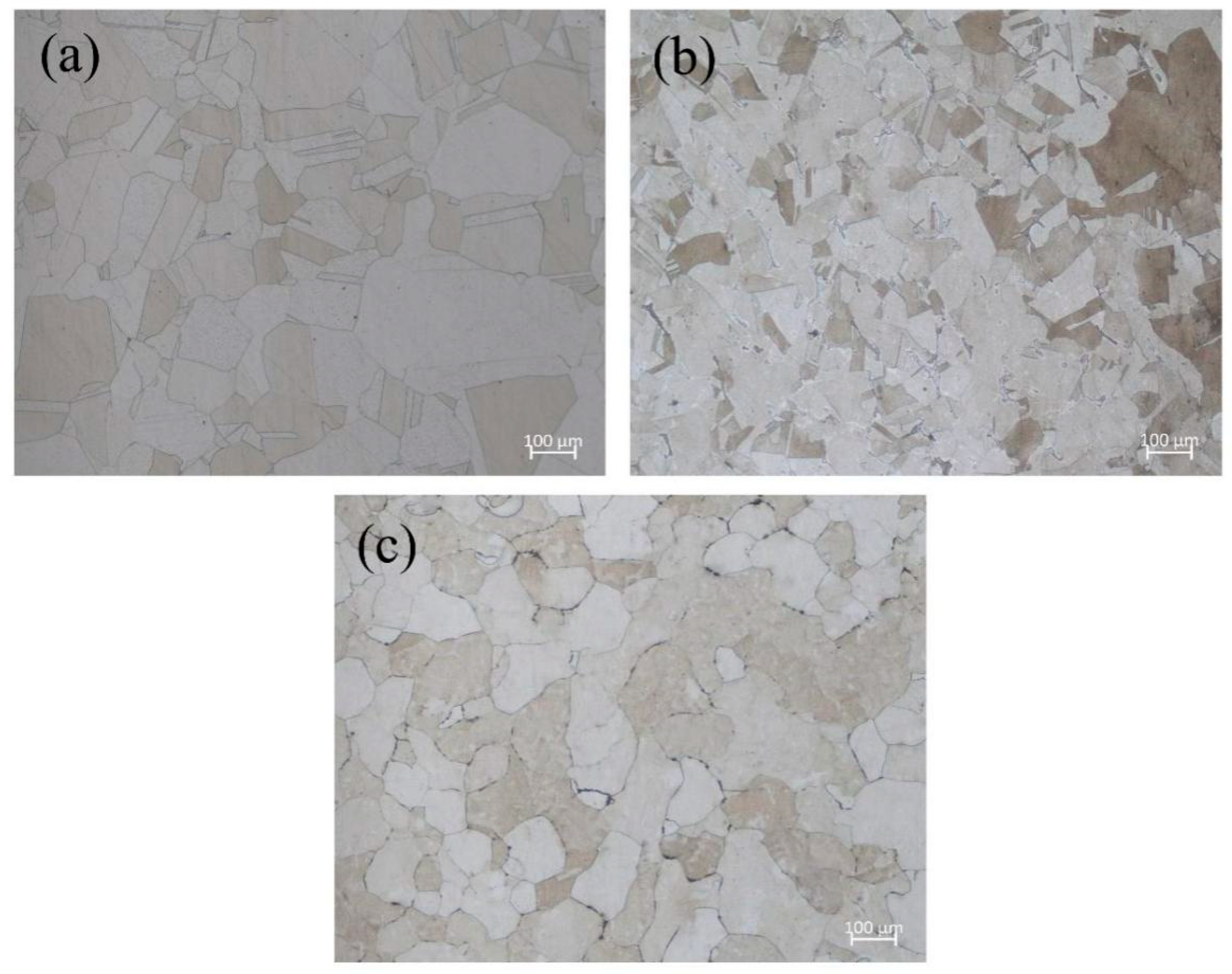
Figure 1.
Optical microscope images of the metallographic microstructure of three materials. (a) 316L stainless steel; (b) 347L stainless steel; (c) Co32Cr28Ni32.94Al4.06Ti3.
2.2. Uniaxial Tensile Test
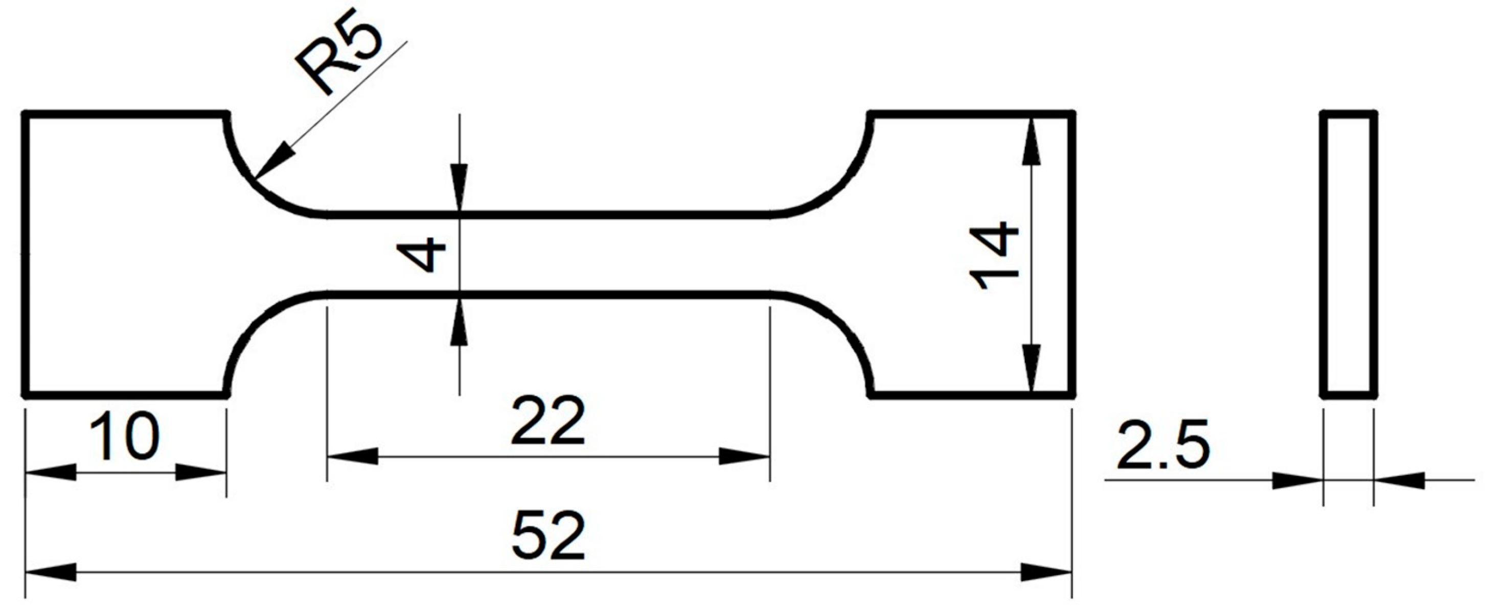
In order to obtain the mechanical properties of the materials, uniaxial tensile tests were carried out at room temperature using AG-X plus a universal electronic testing machine (SHIMADZU corp., Kyoto, Japan), as shown in Figure 2. A 52 mm × 14 mm × 2.5 mm plate-shaped tensile test specimen was used (Figure 3), and tensile tests were carried out at a strain rate of 1 × 10⁻³ mm/s. Finally, the yield stress (σYS), ultimate tensile strength (σUTS), and uniform elongation (ε) of three materials are presented in Table 3.
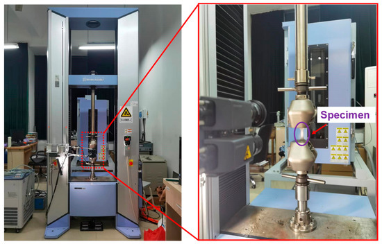
Figure 2.
Overview of uniaxial tensile test.
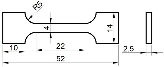
Figure 3.
Dimensions of the tensile specimen (mm).
Table 3.
Mechanical properties of three materials at room temperature.
2.3. Small Punch Test
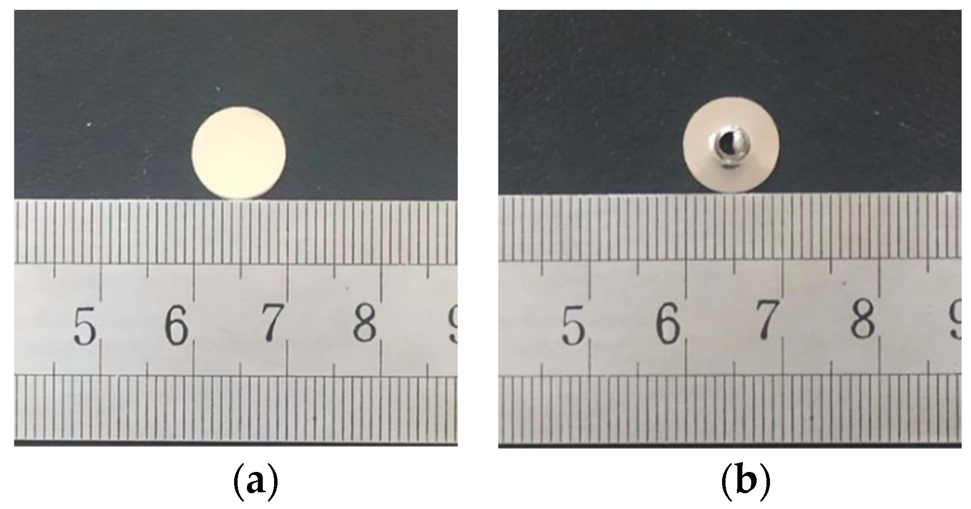
SPT specimens with a diameter of 10 mm and a thickness of 0.8 mm were cut from the plate-shaped tensile specimens after the experiment. Then, the specimens were polished to 0.55 mm on both sides by 600, 1200, and 1500 grit size papers, and finally, the specimens were finely polished to a mirror brightness of 0.5 mm by diamond lapping paste to meet the standard requirements for the surface roughness of the specimens. Figure 4 shows the macroscopic morphology of the small punch specimen before and after the experiment.
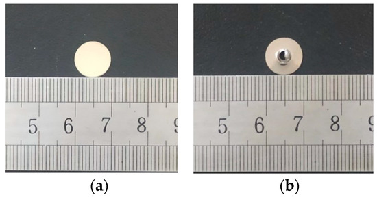
Figure 4.
Macro morphology of a small punch specimen. (a) before test; (b) after test.
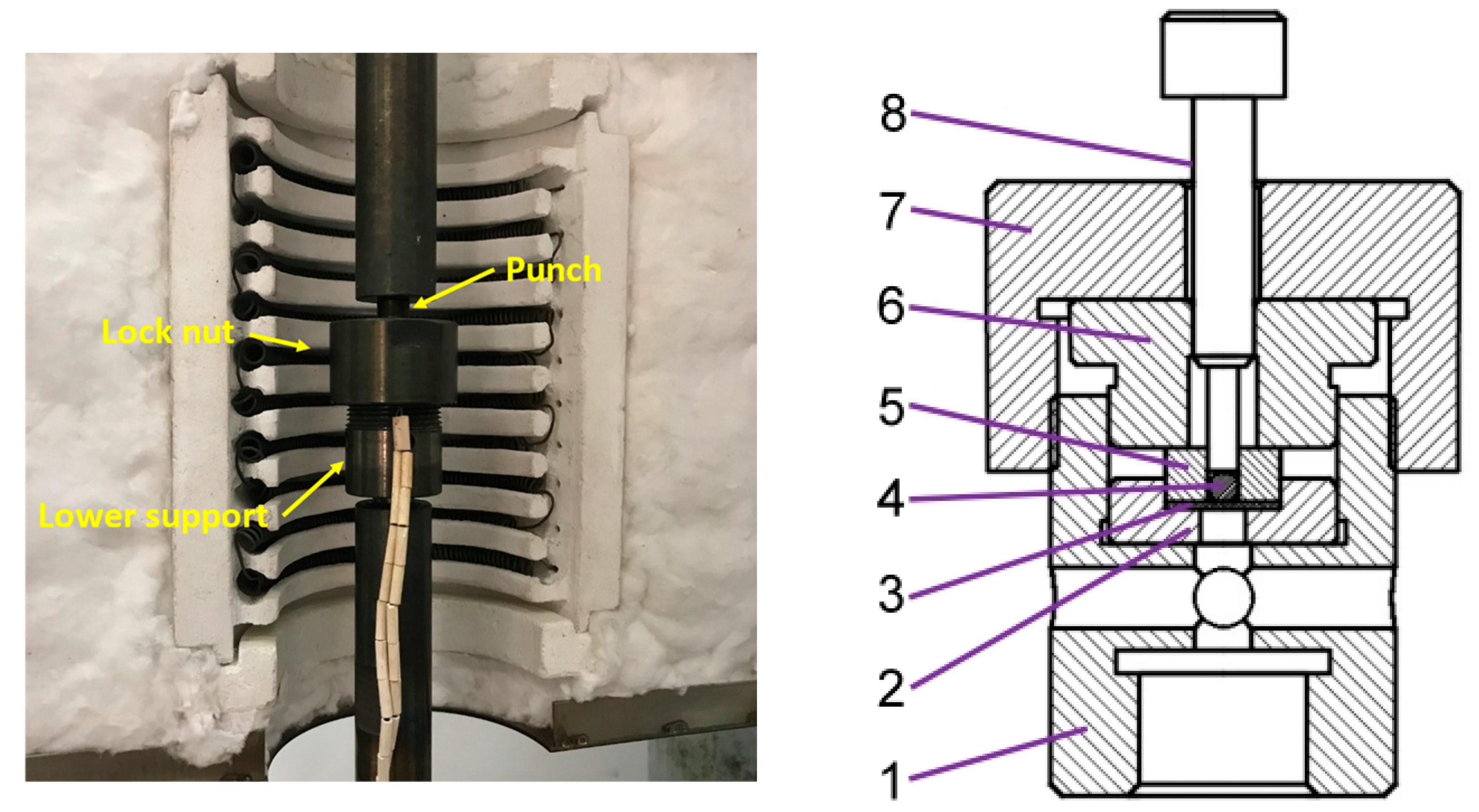
In this paper, the small punch test apparatus, modified based on the small punch creep test machine, was used to conduct SPT. Its force sensor and displacement sensor are coupled to the loading brake, and the force and displacement changes are recorded by loading the punch. Once the force is received on the force sensor, the displacement sensor begins to record the punch displacement data. This displacement sensor can be used to obtain relatively accurate displacement data of the punch on the top. The schematic diagram of the apparatus is shown in Figure 5. The apparatus for clamping the specimen consists of an upper die, and a circular lower die with a hole diameter of 4 mm. The specimen is placed horizontally and perpendicular to the direction of the force. During the test, the loading is applied to the specimen by means of a punch and a ball with a diameter of 2.5 mm. The test was conducted in a quasi-static condition with a displacement rate of 0.5 mm/min.

Figure 5.
Schematic diagram of small punch test. 1. Lower support 2. Lower die 3. Specimen 4. Ball 5. Guide block 6. Upper die 7. Lock nut 8. Punch.
2.4. FE Model and Numerical Simulation
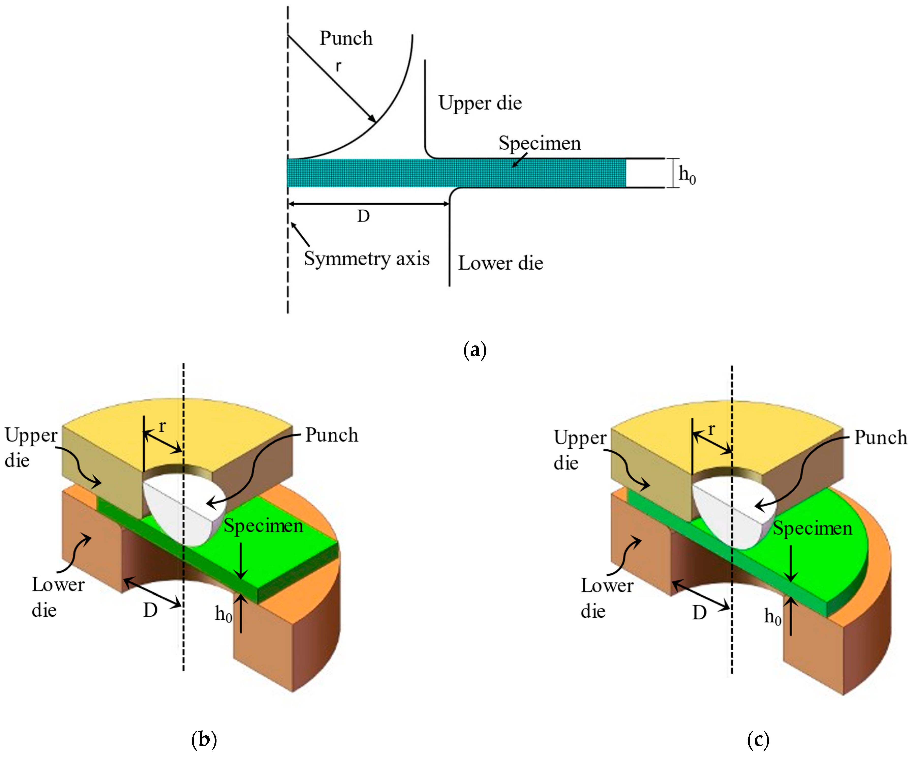
The FE model used in this paper is shown in Figure 6. Both a two-dimensional (2D) axisymmetric model and quarter-symmetric three-dimensional (3D) model were used to simulate the SPT by ABAQUS large commercial FE software [42]. A 2D model with 2000 axisymmetric 4-node square elements, homogenized mesh, and reduced integration with hourglass control (CAX4R) was mainly used to investigate the effect of equipment compliance on experimental data, while a 3D model with about 64,000 8-node linear brick elements, homogenized mesh, and reduced integration with hourglass control (C3D8R) was used to study the effect of specimen size on experimental data. Most researchers widely use these two models in SPT simulations [5,43]. They are suitable for analyzing cases involving large stress and strain gradients, as well as for studying complex contact problems. The agreement between the 2D and 3D model results was confirmed in the article [29,30] by Altstadt et al. Isotropic elastic–plastic materials are subject to the von Mises yield criterion and the corresponding J2 flow theory [44,45], which takes the form as follows,
where σ1, σ2, and σ3 are the three principal stresses respectively. The material properties’ inputs in ABAQUS were imported from real stress–strain data evaluated by uniaxial tensile tests of related materials, as shown in Table 3. The constitutive equation can be expressed in the following form,
where the σp(εp) equation is derived from the uniaxial tensile behavior [32]. Generally, the FE model constructed consists of four parts, namely the (1) punch, (2) upper die, (3) lower die, and (4) specimen. Unlike the test, the FE model perfectly simulates the test setup under ideal conditions. The upper and lower dies and punch are defined as rigid bodies, and the specimen is defined as a deformable body. The upper and lower dies were completely fixed to simulate the clamping condition during the experiment, while the displacement constraint was applied to the punch until the specimen fails. The friction coefficient between the punch and specimen was set to 0.2, which is a typical friction coefficient for steel-steel contact in the absence of lubrication [46]. The equipment dimensions for the SPT test and FE simulation were kept consistent. The relevant parameters of specimens and apparatus for different models are summarized in Table 4. The mesh refinement was performed to ensure the accuracy of simulation results. The mesh sizes of square and round specimens in the 3D model were consistent to avoid the impact of mesh sensitivity on simulation results [47,48].

Figure 6.
Schematic diagram of FE model of SPT. (a) 2D model; (b) 3D model with square specimen; (c) 3D model with round specimen.
Table 4.
Geometric parameters of SPT for 2D and 3D models.
3. Results
3.1. SPT Experiment Results
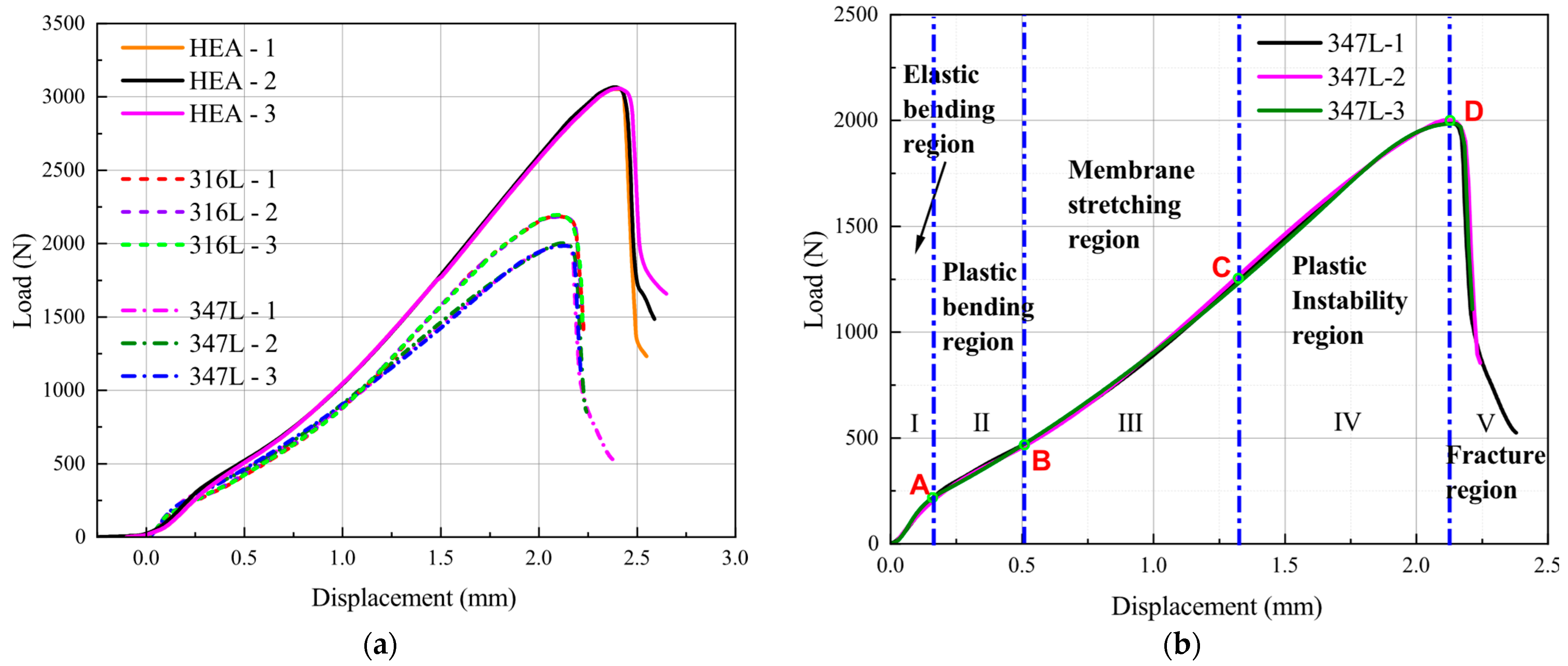
The typical force–displacement responses of the three materials are shown in Figure 7a. Three test groups were analyzed for each material, and the results show a high degree of coincidence of the force–displacement curves. The force–displacement data of the SPT experiment curve was recorded until the force exceeded the maximum force point and after the specimen ruptured.
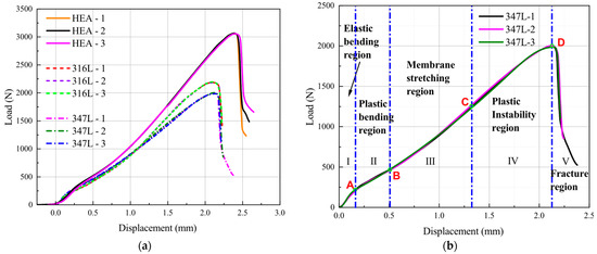
Figure 7.
Force–displacement curve of SPT. (a) The three materials; (b) representation of the different stages.
As shown in Figure 7b, The force–displacement curve can be divided into five different regions: elastic bending (region I), plastic bending (region II), membrane-stretching (region III), plastic instability (region IV), and unstable fracture (region V). However, the boundaries between these five regions are not clearly defined, and the delineation of the different regions is highly artificial. The force in the initial elastic stage (region I) and plastic stage (region II) increases almost linearly, and an obvious inflection point can be seen between the two regions. This inflection point is called the elastic–plastic transition point. The ordinate value corresponding to this point is defined as the elastic–plastic transition force or yield force (FP) (corresponding to point A in Figure 7b) by most researchers, which is usually used to correlate with the yield strength (RP) and regarded as the dividing point between region I and region II. The plastic bending region (region II) ends when the slope of the force–displacement curve increases significantly. In region III, it can be seen that the slope of the force–displacement curve gradually increases. The reason is that after the plastic bending stage, the effect of strain hardening in the material overcomes the reduction of the specimen thickness caused by the punch and enables it to bear the force at an increased rate. This situation is similar to the strain-strengthening stage of the uniaxial tensile test, and the difference is that the stress condition is a biaxial stress state. Therefore, the dividing point between region II and region III (corresponding to point B in Figure 7b) is regarded as the specimen entering the membrane-stretching stage from bending deformation.
The dividing point (corresponding to point C in Figure 7b) between membrane stretching (region III) and plastic instability (region IV) can be regarded as a balance point between the material force bearing and deformation resisting. When the value of force exceeds the value of Point C, due to the decrease in the local thickness of the specimen, the microvoids in the material continuously nucleate, grow, and coalesce, thus inducing microcracks on the specimen surface. On the macro level, the specimen will become softened, and the slope of the force–displacement curve gradually decreases until the maximum force (corresponding to point D in Figure 7b) is reached and the stage of plastic instability (region IV) ends.
Figure 8 shows the SEM images of the three materials observed after the specimens fractured (region V). It can be observed that a large number of dimples formed in the material, and a large number of microvoids coalesced. Then, the force of the specimens begins to drop sharply, which is called an unstable fracture region (region V).
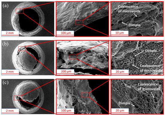
Figure 8.
SEM image for three materials. (a) 316L stainless steel; (b) 347L stainless steel; (c) Co32Cr28Ni32.94Al4.06Ti3.
3.2. SPT Simulation Results
Figure 9a shows the experiment and simulation results of the three materials used in this study. When compared with the experiment results, the dividing points in the force–displacement curve of simulation are more pronounced. The general trends of the experiment and simulation responses are approximately similar in the initial four regions but different in the slopes. This deviation is more pronounced at the initial stage of the force–displacement curve, as shown in Figure 9b. The reason can be explained as that, contrary to the experiment, the specimen dies and punch are defined as rigid bodies in the simulation process, but in fact are elastic deformers. In the practical data recording, different displacement measurement methods lead to the displacement sensor at the top of the punch recording additional displacement due to the elastic deformation of the test frame [39] during the loading process, so that the displacement data recorded by the displacement sensor at the top of the punch (corresponding to SPT test) are slightly higher than the displacement data on the upper face of the specimen (corresponding to SPT simulation). The above situation leads to deviations of the force–displacement curves between the test and simulation. This deviation is also reported in literature [28,32].
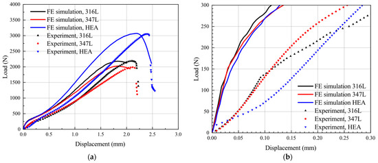
Figure 9.
Comparison of force–displacement curve between the experiment and FE simulation. (a) at all stages; (b) at the initial stage.
3.3. Calibration of Loading System Compliance
In the previous section, we analyzed and explained the reasons for the deviations between the experimental and simulation results. However, the reasonableness of the analytical results for the curves in Figure 9 needs to be further investigated by applying the compliance calibration of the loading system to the experimentally obtained force–displacement curves. It is worth noting that regarding the compliance calibration of the loading system, different compliance calibration methods are used by researchers [27,28,32,39,40,46,49]. The displacement (δupper) on the upper face of the specimen can be derived from the displacements (δext) through an appropriate correction of the respective elastic compliances involved, referred to as Cext [28,32,39,40]. Some researchers [27,43,46] believe that a linear calibration of the force–displacement (δext) response can be achieved with the compliance calibration curve obtained by this method. However, other researchers have argued that the effective contact area with the punch, the applied stress, and the strain field obtained during the SPT are neither constant nor uniform and continuously vary during the test. At the same time, as the punch displacement increases, the deformation of the specimen and the effective contact area of the material increases, and the specimen stiffness gradually increases [27]. Thus, the nonlinear calibration for the force–displacement (δext) response should be considered in the actual compliance calibration to obtain the best match between the test and simulation curves. Meanwhile, Ávila et al. [27] also pointed out that if only the initial stiffness is used to correct the original curve, a large overcorrection may be obtained for high displacement values.
Therefore, a nonlinear compliance calibration curve was used in this paper. The compliance calibration of the loading system was performed using a cylindrical tungsten carbide specimen with a diameter of 10 mm and a thickness of 5 mm instead of the small circular piece in the test. The calibration method is similar to the reference [43]. In the first loading step, the maximum force was obtained, The subsequent force should not be exceeded in the SPT, and some unloading–loading cycles were performed until a steady state of the force–displacement (δext) curve was reached. The last loading step of this calibration test was recorded, and a fifth-order polynomial regression was established from this data as a calibration equation. This curve was used to calibrate the δext obtained from the SPT test, which resulted in a new displacement (δupper) equal to the displacement of the upper surface of the specimen. It should be noted that the high sensitivity of the calibration process on the test apparatus makes the loading–unloading process unstable. Therefore, in addition to the compliance calibration curves obtained in this study, the correction results for AISI 304L by Moreno et al. [39] and the three calibrations for JRQ by Lucon et al. [49] are also shown in Figure 10.
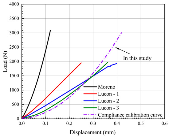
Figure 10.
Compliance calibration curve by different researchers.
As can be seen from the results in Figure 10, the final calibration curves are different due to the displacement measurement systems, test apparatus, and punch materials used by the researchers. It can also be found that the results in the reference [47] show that there are still slight deviations in the three compliance calibration results for the same material with the same test apparatus. Therefore, the compliance calibrations in Appendix A of EN 10,371 [21] are given as a recommended range.
The compliance curve in Figure 10 can be expressed in the following form:
where δΝWC is the elastic deformation of the test apparatus and punch, F is the corresponding force. The force–displacement curve in Figure 7 can also be expressed in the following form:
where δexp includes the elastic bending deformation due to specimen deflection plastic indentation of the punch and elastic deformation of the test frame. Thus, the actual displacement of the specimen can be expressed as:
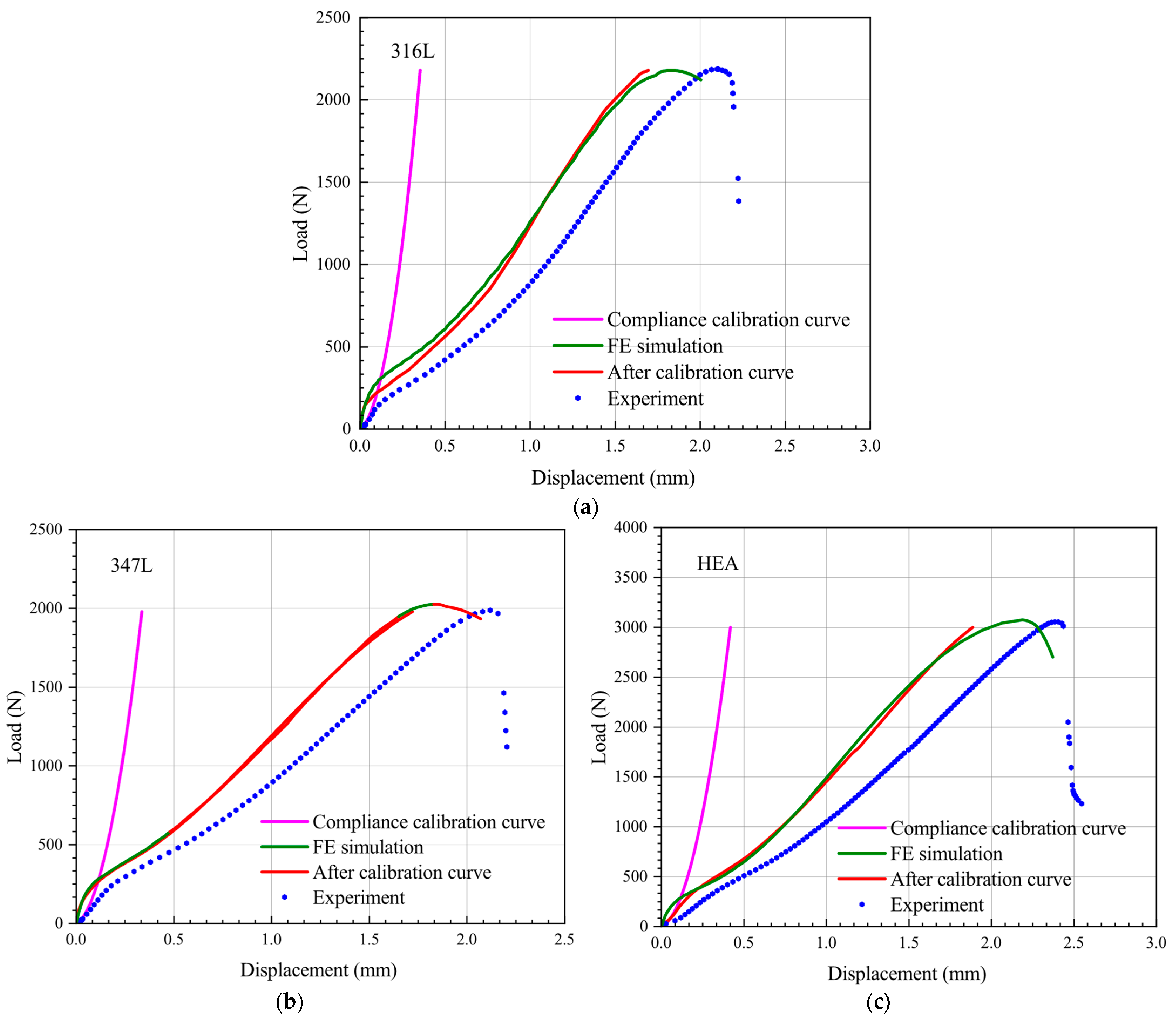
where δupper is the displacement of the upper face of the specimen; the corrected results for the above three materials by Equation (5) are shown in Figure 11. As can be seen, the corrected curves obtained using the above calibration method generally agree well with the simulated curves, with only slight deviations at the initial stages of the curves. Therefore, the deviation between the experiment and simulation results can be attributed to the influence of loading system compliance.
δΝWC = P1(F)
δexp = P2(F)
δupper = δexp − δΝWC = P2(F) − P1(F)
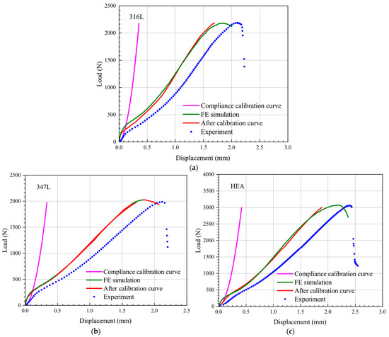
Figure 11.
Force–displacement curve of SPT before and after compliance correction. (a) 316L; (b) 347L; (c) HEA.
4. Discussion
4.1. Correlation between SPT Curve and Tensile Properties before and after Compliance Calibration
The above results confirm that the deviation between experimental and FE results in the displacement is caused by the compliance of the testing machine configuration and the displacement measurement method. It is important to note that due to the high sensitivity of the SPT, the disturbance generated in the process of correcting the compliance of the loading system may lead to the failure of the calibration process, and extra care should be taken in this process. In fact, due to the different displacement measurement methods and materials in the SPT equipment, the results of the compliance calibration are very different. One of the best methods to avoid this problem is to use LVDT contact displacement measurements directly. This method can directly obtain accurate displacement data at the bottom of the specimen and prevent the possible failure of compliance calibration. However, due to the conditions in different laboratories, direct contact displacement measurements sometimes cannot be used. Thus, the effect of testing machine configuration compliance on the empirical correlation results is worth discussing.
4.1.1. Correlation with Ultimate Tensile Strength (σUTS)
Researchers widely use the maximum force (Fm) as the characteristic force associated with the ultimate tensile strength (σUTS). The primary empirical correlation forms are as follows [50]:
where h0 is the specimen’s initial thickness, Fm is the maximum force used to determine the force characteristic value of σUTS, and um is the value of displacement corresponding to the force characteristic Fm. α1, α2, α1’, and α2’ are the correlation coefficients related to the material. The results before and after compliance calibration for the three materials are presented in Table 5.
Table 5.
Characteristic parameters (maximum force) of the SPT curve before and after compliance calibration.
Equations (6) and (7), respectively, were used to empirically correlate the maximum force (Fm) and the ultimate tensile strength (σUTS) of the three materials before and after compliance calibration. Equations (8) and (9) are the empirical correlation equations before compliance calibration and Equations (10) and (11) are the after-compliance calibration equations. The relation between the SPT characteristic force (Fm) and UTT strength property (σUTS) can then be expressed as follows:
Before compliance calibration:
After compliance calibration:
Comparing Equation (8) with Equation (10), it can be seen that the correlation coefficients in the empirical correlation equations obtained from Equation (6) are less affected before and after the compliance calibration and differ only in the correlation coefficient α2. However, it can be seen from the results of the compared Equation (9) with Equation (11) that the correlation coefficients are slightly different before and after compliance calibration. The reason for the above situation is that empirical correlation equation, Equation (6), for each material is only concerned with Fm, which hardly changes before and after the calibration, and thus the difference is not significant. For the same reason, the empirical correlation equation, Equation (7), for each material is not only relevant to Fm but to um, and um changed significantly before and after the calibration, so the data obtained after the compliance calibration of Equation (7) are different from before. Suppose the uncorrected curve is used to evaluate the material ultimate tensile strength (σUTS); an overestimation of results may be obtained (i.e., the larger value of σUTS will be obtained by the uncorrected curve compared with the corrected curve with the same Fm/(h0·um)), and therefore unsafe results will be obtained.
4.1.2. Correlation with Yield Stress (σYS)
The empirical correlation equation of yield stress is usually expressed in the following form,
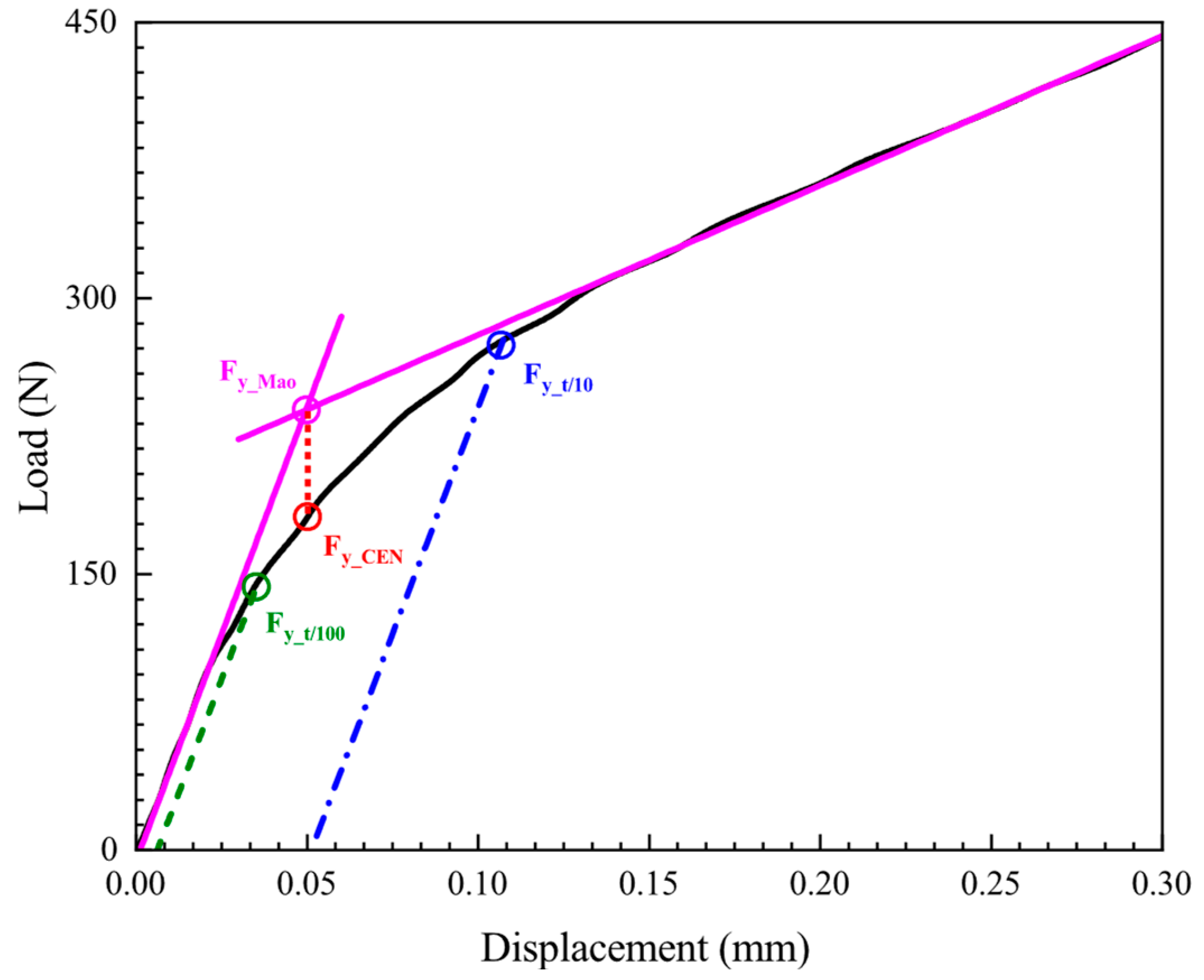
where β1 and β2 are the empirical correlation constants, h0 is the initial thickness of SPT specimen, and Fy is the elastic–plastic transition force in the SPT curve. The key to determining yield stress (σYS) lies in how to determine the corresponding characteristic force, i.e., elastic–plastic transition force (Fy). Different methods for determining Fy are proposed, as described in references [28,50]. In all the current assessments, Fy_Mao [51], Fy_CEN [22], Fy_t/10 [52], and Fy_t/100 [6] methods are adopted by most researchers, as shown in Figure 12.

Figure 12.
Different methods of determining the force Fy on SPT curve.
The Mao method [51] minimizes the error between the linear function and the SPT initial stage curve by establishing two linear procedures, and the resulting intersection point is Fy_ Mao, and the intersection point projected vertically onto the SPT curve is Fy_CEN. The t/10 and t/100 methods were performed by drawing a parallel line tangent to the elastic region I of the SPT curve. The line was translated along the deflection axis to the points whose values are t/10 and t/100, respectively. The intersection value between the parallel line tangent and SPT curve was determined as the characteristic force Fy. The maximum slope of the tangent line corresponding to the slope at the inflection point is suggested in Hähner et al. [40] as the slope of the elastic region I of the SPT curve before compliance calibration, and this method was used in this paper to determine the yield stress (σYS) before compliance calibration.
The characteristic forces (Fy) associated with the yield stress (σYS) before and after the compliance calibration are listed in Table 6. The relation between the SPT characteristic force (Fy) and UTT material property (σYS) can then be expressed as follows:
Table 6.
Characteristic force of the SPT curve determined by different methods before and after compliance calibration (yield force).
Before compliance calibration:
After compliance calibration
where Equations (13)–(16) as well as Equations (17)–(20) correspond to the four methods for determining Fy, respectively. A comparison of the empirical correlation coefficients in the equations above intuitively shows that the differences before and after the compliance correction are obvious for different methods of determining the yield force (Fy). The empirical correlation equations before and after compliance calibration determined using Fy_Mao, Fy_CEN, and Fy_t/10 methods showed small deviations, and the empirical correlation coefficients β1 and β2 do not differ significantly. In contrast, the empirical correlation equations determined by the Fy_t/100 method showed larger deviations in the empirical correlation coefficients β1 and β2 before and after compliance calibration, which indicates that the Fy_Mao, Fy_CEN, and Fy_t/10 methods are less affected by the compliance calibration and are more applicable to the characteristic forces of the above-mentioned study materials.
It can also be seen that the regression coefficient R2 of the empirical correlation equation for yield strength (σYS) is relatively small compared to the empirical correlation equation for ultimate tensile strength (σUTS), indicating that its empirical correlation equation has a large scattering, which may be caused by the small number of data points. Table 6 illustrates the values of the empirical correlation constant β1 from the literature of different researchers. It should be noted that for the empirical correlation equation of yield strength, the coefficient β2 may not necessarily exist, depending on the differences in the mechanical properties of the material and the influence of the test apparatus. Table 7 combined with Equations (17) and (18) shows that the values of β1 determined by the Mao and CEN methods are close to the values in the literature [5,32,41,42,43,44,45,46,47,48,49,50,51,52,53]. Therefore, by combining the two perspectives above, Fy_Mao and Fy_CEN may be the more desirable characteristic forces for the three materials of interest in this study.
Table 7.
Recommended values of parameters β1 and β2 in different literature.
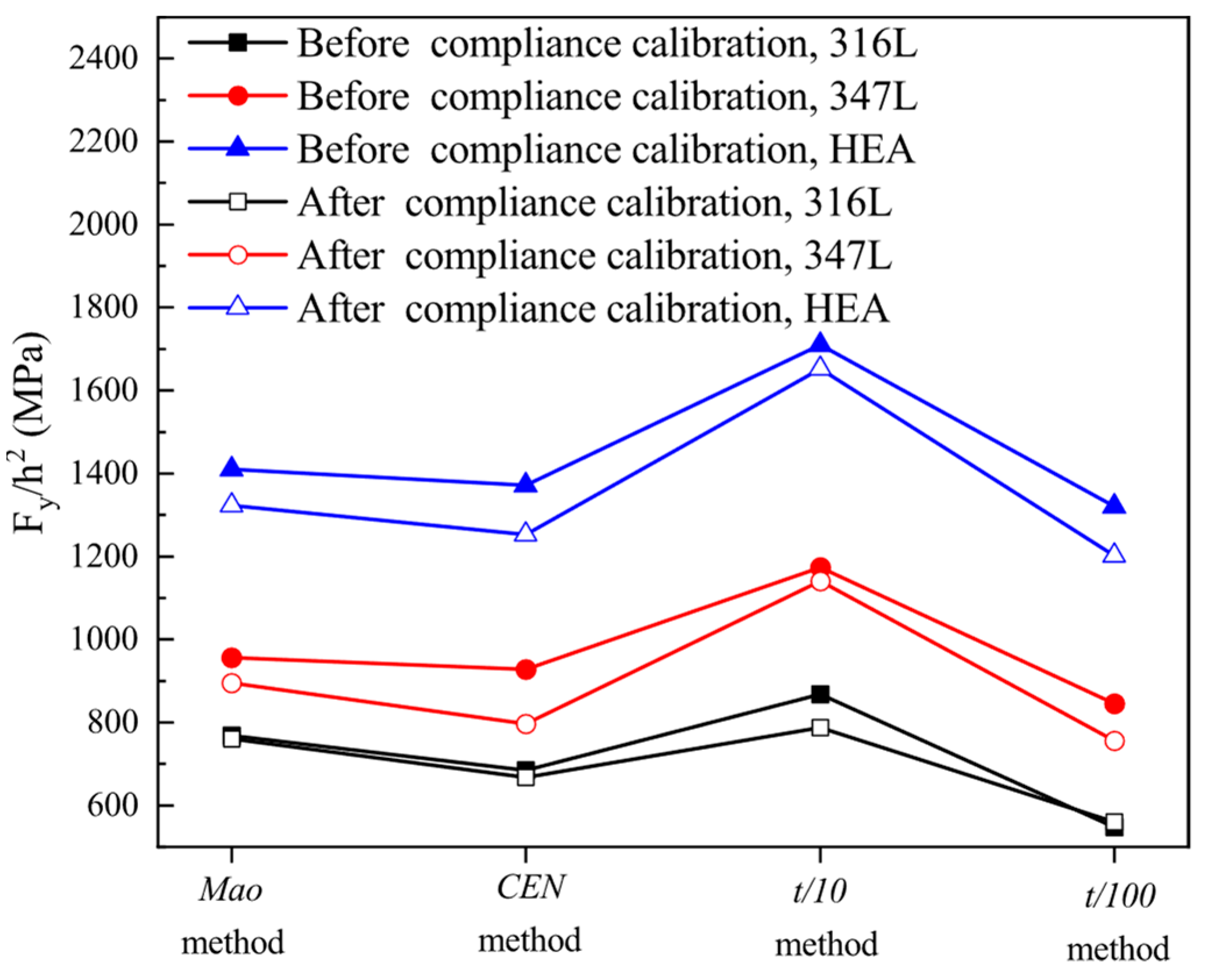
Figure 13 compares the different methods of determining the yield force (Fy) for the three materials studied in this paper. It can be seen that the difference in the methods of determining the yield force (Fy) before and after compliance correction is slight. This result indicates that the determination of the yield stress (σYS) is not affected by the loading system stiffness. It can also be seen that if the empirical correlation coefficient in Equation (8) is constant, the t/10 method obtains the highest yield strength of the material, while the other three methods obtain the yield strength of the material relatively close. However, this result was demonstrated only for the three materials studied in this paper, and its applicability to other materials remains further confirmed.

Figure 13.
Different methods for determining the Fy.
4.2. Effect of Different Specimen Sizes on SPT Curve
In order to avoid the influence of some neglected factors on the SPT results during the experiments, the subsequent studies of different specimen sizes were based on FE analysis. The different specimen sizes generally used by most researchers are presented in Table 8. The data of 316L stainless steel mentioned above were used for FE simulations. The mesh sizes of square specimens and round specimens in the 3D model were identical to avoid the impact of mesh sensitivity on simulation results.
Table 8.
FE model parameters of 316L stainless steel with different specimen sizes.
Figure 14 shows the results of the SPT curves for all cases in Table 7. It can be seen that the FE simulation results for round and square specimens with the same diameter exhibit almost identical SPT curves. This result shows that the SPT curves were not influenced by the specimen’s shape when the specimen periphery was in a fully clamped condition. Moreover, for specimens with diameters of 8 mm and 10 mm, respectively, there is a high degree of coincidence in the first four regions of the SPT curves. Still, the two curves begin to diverge near the maximum force, and the general downward trend in force remains consistent beyond the maximum force. In general, the effect of specimens’ diameter on the force–displacement curve is not apparent, and a slight difference induced by the specimen diameter can be found beyond the maximum force point.
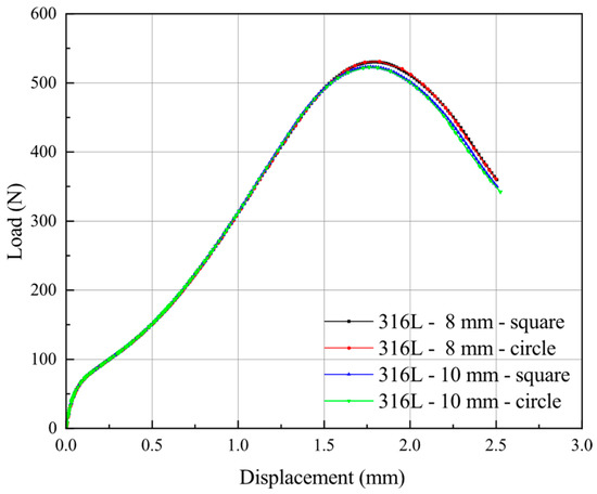
Figure 14.
Force–displacement curve of SPT test for specimens in Table 7.
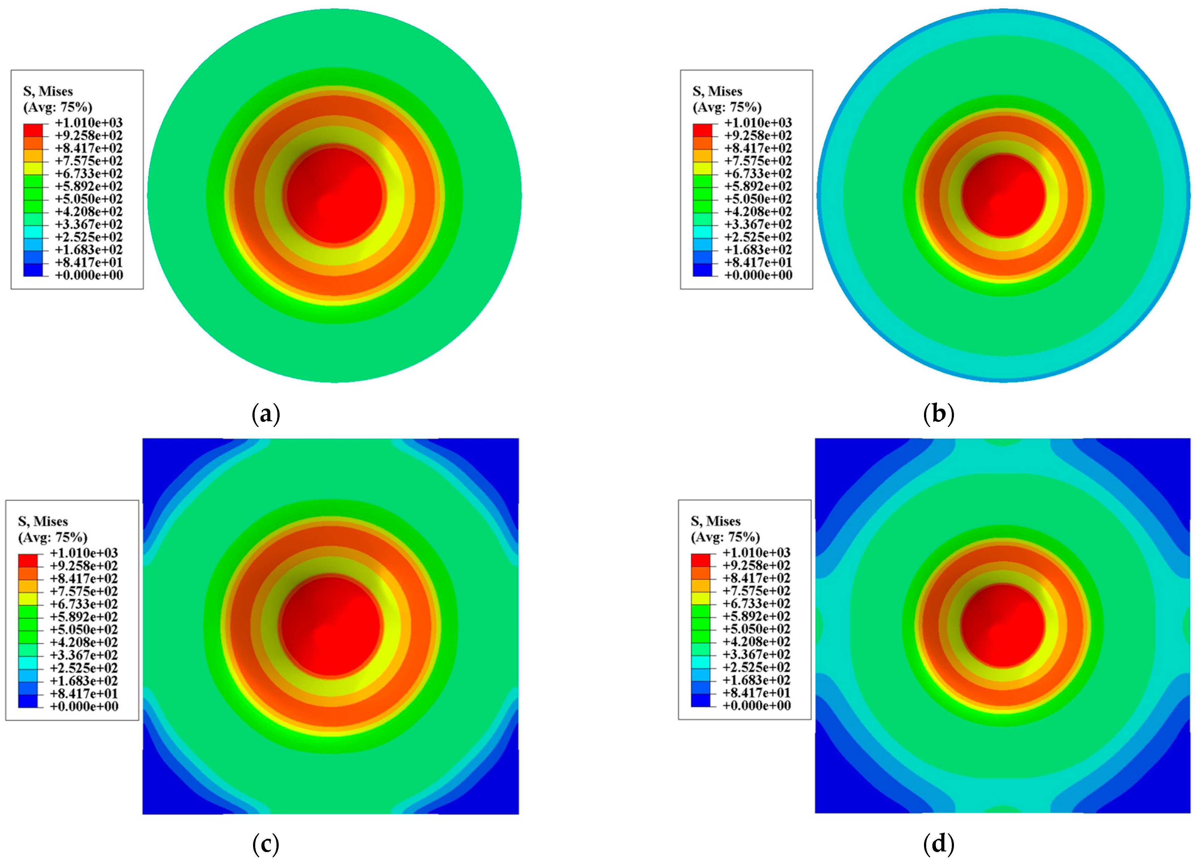
Figure 15 shows the equivalent stress distribution of four different types of specimens of 316L stainless steel when the punch displacement was 1.7 mm. It can be seen from the figure that although the overall stress distribution of square specimens and round specimens is different, the stress distribution of the contact part with the punch at the center of the specimen is roughly the same. The difference between round or square specimens with different diameters is only evident in the non-contact area with the punch.

Figure 15.
Contour plots for Von Mises stress on FE model of SPT. (a) round specimen with a diameter of 8 mm; (b) round specimen with a diameter of 10 mm; (c) square specimen with a diameter of 8 mm; (d) square specimen with a diameter of 10 mm.
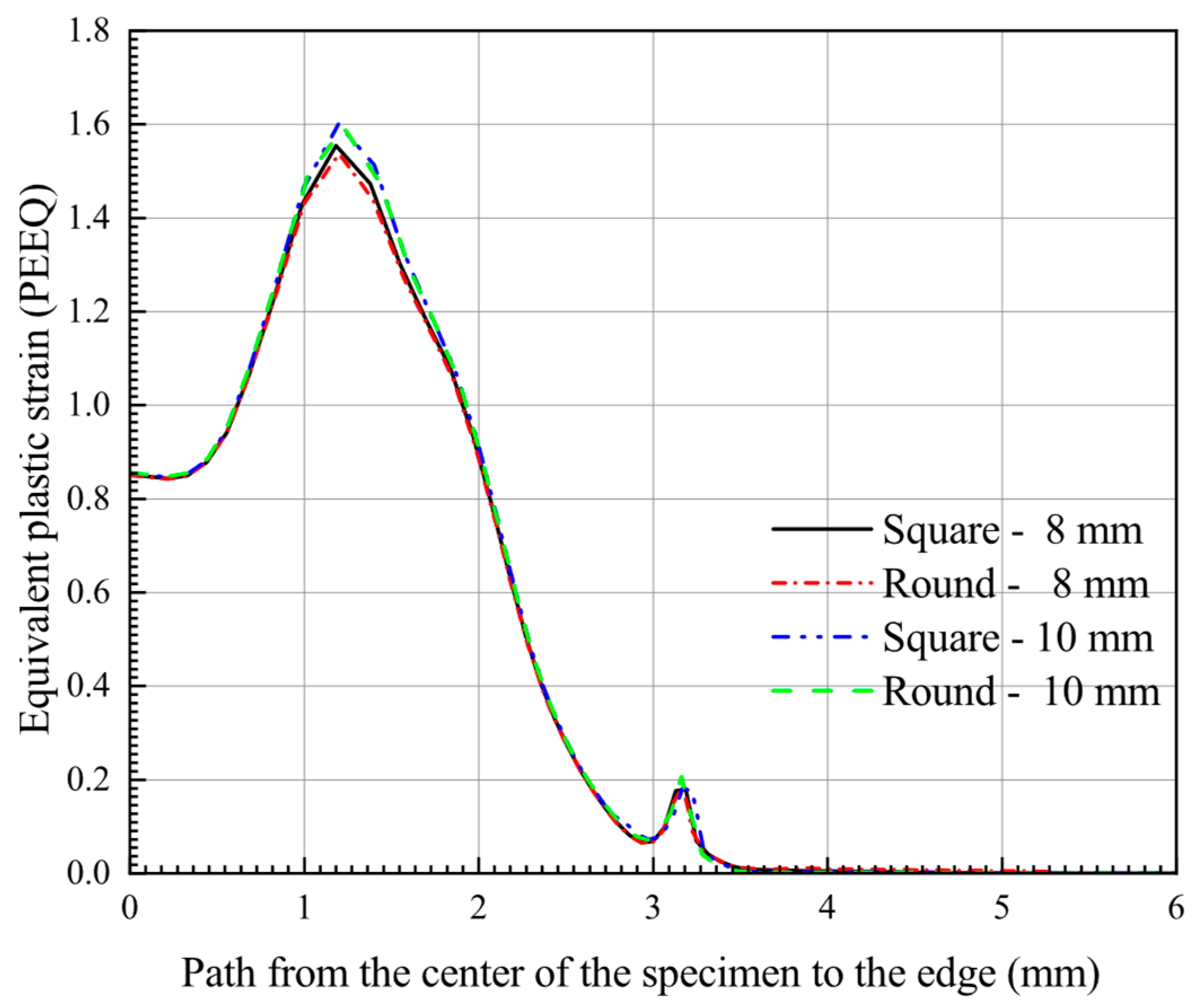
Figure 16 shows the equivalent plastic strain distribution on the bottom surface of the specimen at the maximum force in the path from the center of the specimen to the edge. Combined with the contour plots of the equivalent plastic strain distribution for specimens of different diameters and shapes in Figure 15, it can be more intuitively seen that the different specimen sizes have almost the same equivalent plastic strain distributions for the SPT deformation process.
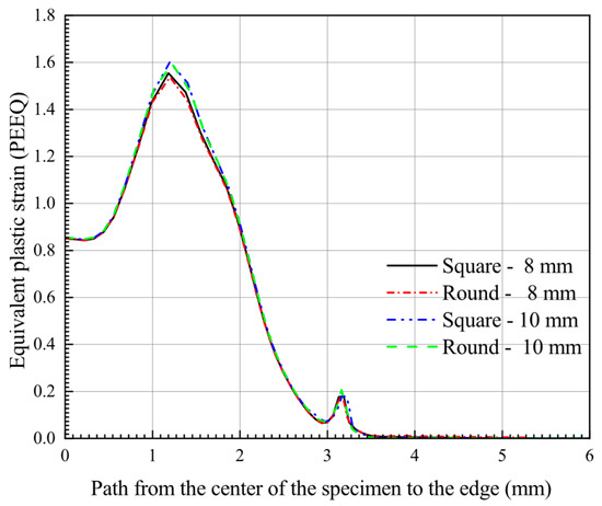
Figure 16.
PEEQ distribution on the bottom surface of the specimen at the maximum force in the path from the center of the specimen to the edge.
Based on the above results, it can be seen that different specimen sizes, i.e., round and square specimens with different diameters kept clamped around, have little effect on the SPT curve results. This implies that the results obtained are theoretically transferable and comparable when SPT tests are performed by different researchers using square and circular specimens, respectively. However, this conclusion must be carried out under the condition that the periphery of the specimen is wholly clamped in the experimental results.
5. Conclusions
In this paper, SPT experiments and simulations were carried out on 316L, 347L stainless steels, and a new high-entropy alloy Co32Cr28Ni32.94Al4.06Ti3, and the effect of specimen sizes on the SPT curve were investigated by simulation. The main conclusions are as follows:
(1) The discrepancy of the force–displacement of SPT between the test and the simulation results is mainly due to the loading system stiffness.
(2) The empirical correlation results for the ultimate tensile strength (σUTS) by Equation (6) and for the yield strength (σYS) by Equation (12) have little difference before and after the loading system compliance calibration, but the correlation results by Equation (7) have a greater difference because of the changes in um before and after the loading system compliance calibration.
(3) Simulation results on different specimen shapes and sizes show that the effect of specimen shapes and sizes on the SPT results can be ignored. This conclusion was confirmed by the 316L stainless steel simulation results. Therefore, the experimental results obtained based on the above specimen size provide a reference for different researchers even if their specimen shapes and sizes differ.
This investigation shows that insufficient stiffness of a loading system can lead to an inaccurate material properties by the small punch test, but the results after correction are still trustworthy. It also provides a reference for subsequent researchers to conduct empirical correlation studies using different specimen sizes.
Author Contributions
Conceptualization, J.Z. and Z.G.; methodology, J.Z. and Z.G.; software, Z.G.; validation, J.Z. and Z.G.; formal analysis, Z.G.; investigation, J.Z., Z.G. and K.L.; data curation, Z.G.; writing—original draft preparation, Z.G.; writing—review and editing, J.Z. and Z.G.; visualization, J.Z. and K.L.; supervision, K.L.; project administration, J.Z. and K.L.; funding acquisition, J.Z. All authors have read and agreed to the published version of the manuscript.
Funding
This research was funded by National Natural Science Foundation of China (No.51705079), Natural Science Foundation of Fujian Province (No.2018J01767).
Institutional Review Board Statement
Not applicable.
Informed Consent Statement
Not applicable.
Data Availability Statement
Not applicable.
Conflicts of Interest
The authors declare no conflict of interest.
References
- Manahan, M.P.; Argon, A.S.; Harling, O.K. The development of a miniaturized disk bend test for the determination of postirradiation mechanical properties. J. Nucl. Mater. 1981, 104, 1545–1550. [Google Scholar] [CrossRef]
- Nowik, K.; Oksiuta, Z. Experimental and numerical small punch tests of the 14Cr ODS ferritic steel. Acta Mechanica et Automatica 2022, 16, 225–232. [Google Scholar] [CrossRef]
- Bruchhausen, M.; Holmström, S.; Simonovski, I.; Austin, T.; Lapetite, J.M.; Ripplinger, S.; de Haan, F. Recent developments in small punch testing: Tensile properties and DBTT. Theor. Appl. Fract. Mech. 2016, 86, 2–10. [Google Scholar] [CrossRef]
- Cheng, Z.Y.; Sun, J.R.; Tai, P.F.; Zhang, L.Q.; Wei, Y.T.; Chang, H.L.; Thuku, R.; Gichuhi, K.M. Comparative Study between Small Punch Tests and Finite Element Analysis of Miniature Steel Specimens. J. Mater. Eng. Perform. 2021, 30, 9094–9107. [Google Scholar] [CrossRef]
- Cao, Y.; Zu, Y.; Zhen, Y.; Li, F.; Wu, G. Determination of the true stress-strain relations of high-grade pipeline steels based on small punch test correlation method. Int. J. Pres. Ves. Pip. 2022, 199, 104739. [Google Scholar] [CrossRef]
- Contreras, M.A.; Rodriguez, C.; Belzunce, F.J.; Betegon, C. Use of the small punch test to determine the ductile-to-brittle transition temperature of structural steels. Fatigue Fract. Eng. Mater. Struct. 2008, 31, 727–737. [Google Scholar] [CrossRef]
- Ha, J.S.; Fleury, E. Small punch tests to estimate the mechanical properties of steels for steam power plant: II. Fracture toughness. Int. J. Pres. Ves. Pip. 1998, 75, 707–713. [Google Scholar] [CrossRef]
- Lancaster, R.J.; Jeffs, S.P.; Illsley, H.W.; Argyrakis, C.; Hurst, R.C.; Baxter, G.J. Development of a novel methodology to study fatigue properties using the small punch test. Mater. Sci. Eng. A 2019, 748, 21–29. [Google Scholar] [CrossRef]
- Zhao, L.; Wang, X.; Xu, L.Y.; Han, Y.D.; Jing, H.Y. Fatigue performance of Hastelloy X at elevated temperature via small punch fatigue test. Theor. Appl. Fract. Mech. 2021, 116, 103118. [Google Scholar] [CrossRef]
- Lewis, D.T.S.; Lancaster, R.J.; Jeffs, S.P.; Illsley, H.W.; Davies, S.J.; Baxter, G.J. Characterising the fatigue performance of additive materials using the small punch test. Mater. Sci. Eng. A 2019, 754, 719–727. [Google Scholar] [CrossRef]
- Yang, Z.; Wang, Z.W. Relationship between strain and central deflection in small punch creep specimens. Int. J. Pres. Ves. Pip. 2003, 80, 397–404. [Google Scholar] [CrossRef]
- Rouse, J.P.; Cortellino, F.; Sun, W.; Hyde, T.H.; Shingledecker, J. Small punch creep testing: Review on modelling and data interpretation. Mater. Sci. Technol. 2013, 29, 1328–1345. [Google Scholar] [CrossRef]
- Dymáček, P. Recent developments in small punch testing: Applications at elevated temperatures. Theor. Appl. Fract. Mech. 2016, 86, 25–33. [Google Scholar] [CrossRef]
- Yoon, K.B.; Nguyen, T.T. Estimation of high-temperature fracture parameters for small punch specimen with a surface crack. Fatigue Fract. Eng. Mater. Struct. 2018, 41, 1224–1236. [Google Scholar] [CrossRef]
- Nguyen, T.T.; Yoon, K.B. Fully plastic J-integral and C* equations for small punch test specimen with a surface crack. Int. J. Pres. Ves. Pip. 2020, 188, 104214. [Google Scholar] [CrossRef]
- Li, Y.Z.; Dymacek, P.; Hurst, R.; Stevens, P. A novel methodology for determining creep crack initiation and growth properties using FEM with notched small punch specimens. Theor. Appl. Fract. Mech. 2021, 116, 103112. [Google Scholar] [CrossRef]
- Chittibabu, V.; Rao, K.S.; Rao, P.G. Factors affecting the mechnical properties of compact bone and miniature specimen test techniques: A review. Adv. Sci. Technol. Res. J. 2016, 10, 169–183. [Google Scholar] [CrossRef]
- Gulcimen, B.; Hahner, P. Determination of creep properties of a P91 weldment by small punch testing and a new evaluation approach. Mater. Sci. Eng. A 2013, 588, 125–131. [Google Scholar] [CrossRef]
- Wen, W.; Jackson, G.A.; Li, H.; Sun, W. An experimental and numerical study of a CoNiCrAlY coating using miniature specimen testing techniques. Int. J. Mech. Sci. 2019, 157, 348–356. [Google Scholar] [CrossRef]
- Soltysiak, S.; Selent, M.; Roth, S.; Abendroth, M.; Hoffmann, M.; Biermann, H.; Kuna, M. High-temperature small punch test for mechanical characterization of a nickel-base super alloy. Mater. Sci. Eng. A 2014, 613, 259–263. [Google Scholar] [CrossRef]
- EN 10371; Metallic Materials–Small Punch Test Method. European Committee for Standardization: Brussel, Belgium, 2021.
- CWA 15627; Small Punch Test method for Metallic Materials. European Committee for Standardization: Brussel, Belgium, 2007.
- GB/T 29459.1; Small Punch Test Methods of Metallic Materials for In-Service Pressure Equipments—Part 1: General Requirements. Chinese Standard: Beijing, China, 2012.
- GB/T 29459.2; Small Punch Test Methods of Metallic Materials for In-Service Pressure Equipments—Part 2: Method of Test for Tensile Properties at Room Temperature. Chinese Standard: Beijing, China, 2012.
- ASTM E3205; Standard Test Method for Small Punch Testing of Metallic Materials. ANSI: New York, NY, USA, 2022.
- Kalidindi, S.R.; Abusafieh, A.; El-Danaf, E. Accurate characterization of machine compliance for simple compression testing. Exp. Mech. 1997, 37, 210–215. [Google Scholar] [CrossRef]
- Sánchez-Ávila, D.; Orozco-Caballero, A.; Martinez, E.; Portoles, L.; Barea, R.; Carreno, F. High-accuracy compliance correction for nonlinear mechanical testing: Improving Small Punch Test characterization. Nucl. Mater. Energy 2021, 26, 100914. [Google Scholar] [CrossRef]
- Janca, A.; Siegl, J.; Hausild, P. Small punch test evaluation methods for material characterisation. J. Nucl. Mater. 2016, 481, 201–213. [Google Scholar] [CrossRef]
- Altstadt, E.; Houska, M.; Simonovski, I.; Bruchhausen, M.; Holmström, S.; Lacalle, R. On the estimation of ultimate tensile stress from small punch testing. Int. J. Mech. Sci. 2018, 136, 85–93. [Google Scholar] [CrossRef]
- Altstadt, E.; Ge, H.E.; Kuksenko, V.; Serrano, M.; Houska, M.; Lasan, M.; Bruchhausen, M.; Lapetite, J.M.; Dai, Y. Critical evaluation of the small punch test as a screening procedure for mechanical properties. J. Nucl. Mater. 2016, 472, 186–195. [Google Scholar] [CrossRef]
- Lucas, G.E.; Okada, A.; Kiritani, M. Parametric analysis of the disc bend test. J. Nucl. Mater. 1986, 141, 532–535. [Google Scholar] [CrossRef]
- Campitelli, E.N.; Spatig, P.; Bonade, R.; Hoffelner, W.; Victoria, M. Assessment of the constitutive properties from small ball punch test: Experiment and modeling. J. Nucl. Mater. 2004, 335, 366–378. [Google Scholar] [CrossRef]
- Xu, T.; Guan, K.S.; Wang, Z.W. Study on standardization of small punch test (1)—general requirements. Press. Vessel. Technol. 2010, 27, 37–46. (In Chinese) [Google Scholar]
- Zhou, Z.X.; Ling, X. Ductile Damage Analysis for Small Punch Specimens of Type 304 Stainless Steel Based on GTN Model. J. Test. Eval. 2009, 37, 538–544. [Google Scholar]
- Andrés, D.; Dymacek, P. Study of the upper die clamping conditions in the small punch test. Theor. Appl. Fract. Mech. 2016, 86, 117–123. [Google Scholar] [CrossRef]
- Peng, J.; Vijayanand, V.D.; Knowles, D.; Truman, C.; Mostafavi, M. The sensitivity ranking of ductile material mechanical properties, geometrical factors, friction coefficients and damage parameters for small punch test. Int. J. Pres. Ves. Pip. 2021, 193, 104468. [Google Scholar] [CrossRef]
- Moreno, M.F. Effects of thickness specimen on the evaluation of relationship between tensile properties and small punch testing parameters in metallic materials. Mater. Des. 2018, 157, 512–522. [Google Scholar] [CrossRef]
- Peng, J.; Zhang, H.; Wang, Y.Q.; Richardson, M.; Liu, X.D.; Knowles, D.; Mostafavi, M. Correlation study on tensile properties of Cu, CuCrZr and W by small punch test and uniaxial tensile test. Fusion Eng. Des. 2022, 177, 113061. [Google Scholar] [CrossRef]
- Moreno, M.F.; Bertolino, G.; Yawny, A. The significance of specimen displacement definition on the mechanical properties derived from Small Punch Test. Mater. Des. 2016, 95, 623–631. [Google Scholar] [CrossRef]
- Hähner, P.; Soyarslan, C.; Cakan, B.G.; Bargmann, S. Determining tensile yield stresses from Small Punch tests: A numerical-based scheme. Mater. Des. 2019, 182, 107974. [Google Scholar] [CrossRef]
- Guo, J.Q.; Tang, C.Z.Z.; Lai, H.S. Microstructure and Mechanical Properties of Co32Cr28Ni32.94Al4.06Ti3 High-Entropy Alloy. Materials 2022, 15, 1444. [Google Scholar] [CrossRef]
- ABAQUS Users Manual, Version 6.10-1; Dassault Systemes Simulia Corp.: Providence, RI, USA, 2010.
- Chica, J.C.; Diez, P.M.B.; Calzada, M.P. Development of an improved prediction method for the yield strength of steel alloys in the Small Punch Test. Mater. Des. 2018, 148, 153–166. [Google Scholar] [CrossRef]
- Barsanescu, P.D.; Comanici, A.M. von Mises hypothesis revised. Acta. Mech. 2017, 228, 433–446. [Google Scholar] [CrossRef]
- Von Mises, R. Mechanik der festen Körper im plastisch deformablen Zustand. Nachrichten von der Gesellschaft der Wissenschaften zu Göttingen, Mathematisch-Physikalische Klasse 1913, 1913, 582–592. [Google Scholar]
- Chica, J.C.; Diez, P.M.B.; Calzada, M.P. Improved correlation for elastic modulus prediction of metallic materials in the Small Punch Test. Int. J. Mech. Sci. 2017, 134, 112–122. [Google Scholar] [CrossRef]
- Alshboul, O.; Almasabha, G.; Shehadeh, A.; Al Hattamleh, O.; Almuflih, A.S. Optimization of the Structural Performance of Buried Reinforced Concrete Pipelines in Cohesionless Soils. Materials 2022, 15, 4051. [Google Scholar] [CrossRef]
- Almasabha, G.; Alshboul, O.; Shehadeh, A.; Almuflih, A.S. Machine Learning Algorithm for Shear Strength Prediction of Short Links for Steel Buildings. Buildings 2022, 12, 775. [Google Scholar]
- Lucon, E.; Benzing, J.; Hrabe, N. Development and Validation of Small Punch Testing at NIST; US Department of Commerce National Institute of Standards and Technology: Gaithersburg, MD, USA, 2020.
- Garcia, T.E.; Rodriguez, C.; Belzunce, F.J.; Suarez, C. Estimation of the mechanical properties of metallic materials by means of the small punch test. J. Alloys Compd. 2014, 582, 708–717. [Google Scholar] [CrossRef]
- Mao, X.Y.; Takahashi, H. Development of a Further-Miniaturized Specimen of 3 Mm Diameter for Tem Disk (Phi-3 Mm) Small Punch Tests. J. Nucl. Mater. 1987, 150, 42–52. [Google Scholar] [CrossRef]
- Rodriguez, C.; Cabezas, J.G.; Cardenas, E.; Belzunce, F.J.; Betegon, C. Mechanical Properties Characterization of Heat-Affected Zone Using the Small Punch Test. Weld. J. 2009, 88, 188–192. [Google Scholar]
- Lancaster, R.J.; Jeffs, S.P.; Haigh, B.J.; Barnard, N.C. Derivation of material properties using small punch and shear punch test methods. Mater. Des. 2022, 215, 110473. [Google Scholar] [CrossRef]


Publisher’s Note: MDPI stays neutral with regard to jurisdictional claims in published maps and institutional affiliations. |
© 2022 by the authors. Licensee MDPI, Basel, Switzerland. This article is an open access article distributed under the terms and conditions of the Creative Commons Attribution (CC BY) license (https://creativecommons.org/licenses/by/4.0/).