Magnetic Structure of Wiegand Wire Analyzed by First-Order Reversal Curves


Abstract
:1. Introduction
2. Materials and Methods
3. Results
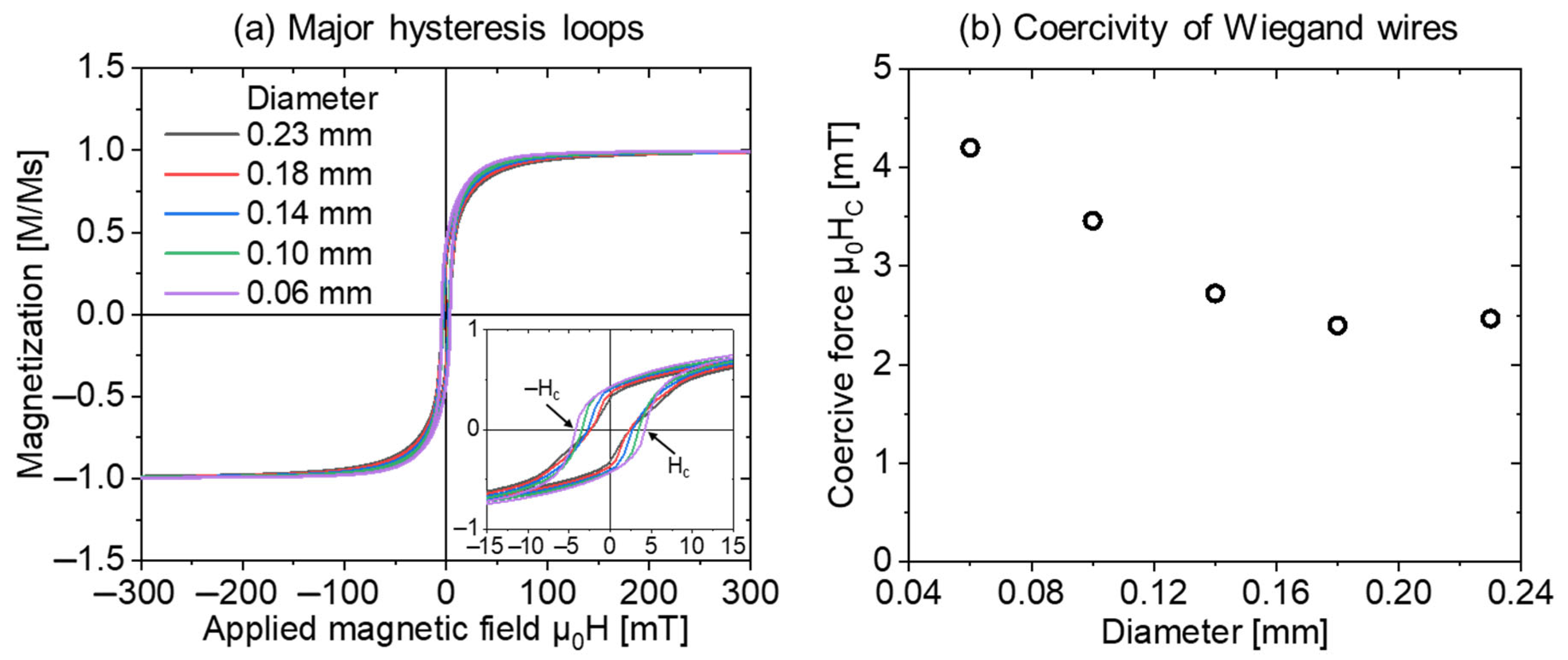
3.1. Major Hysteresis Loops
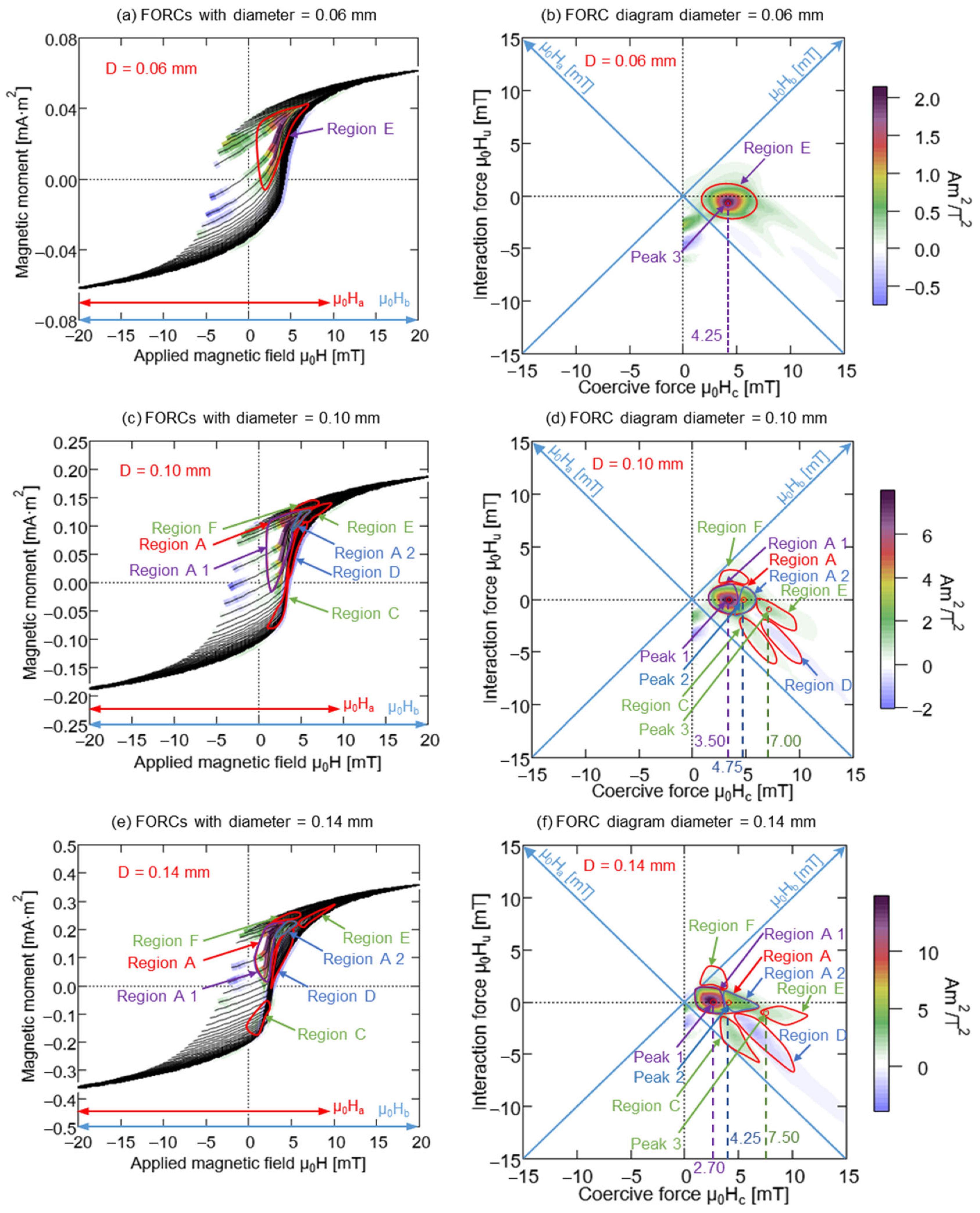
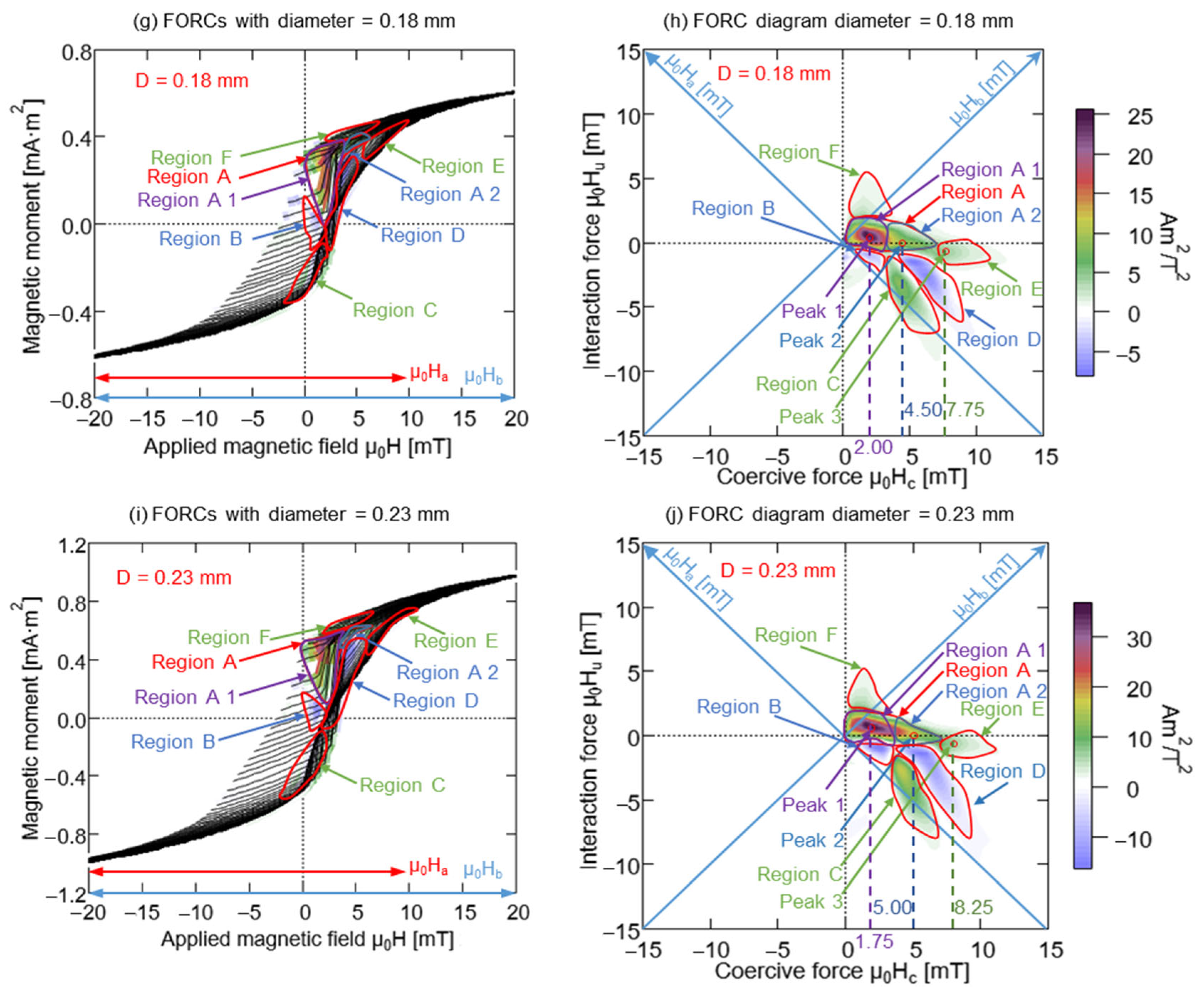
3.2. FORC Curves and FORC Diagrams
4. Discussion
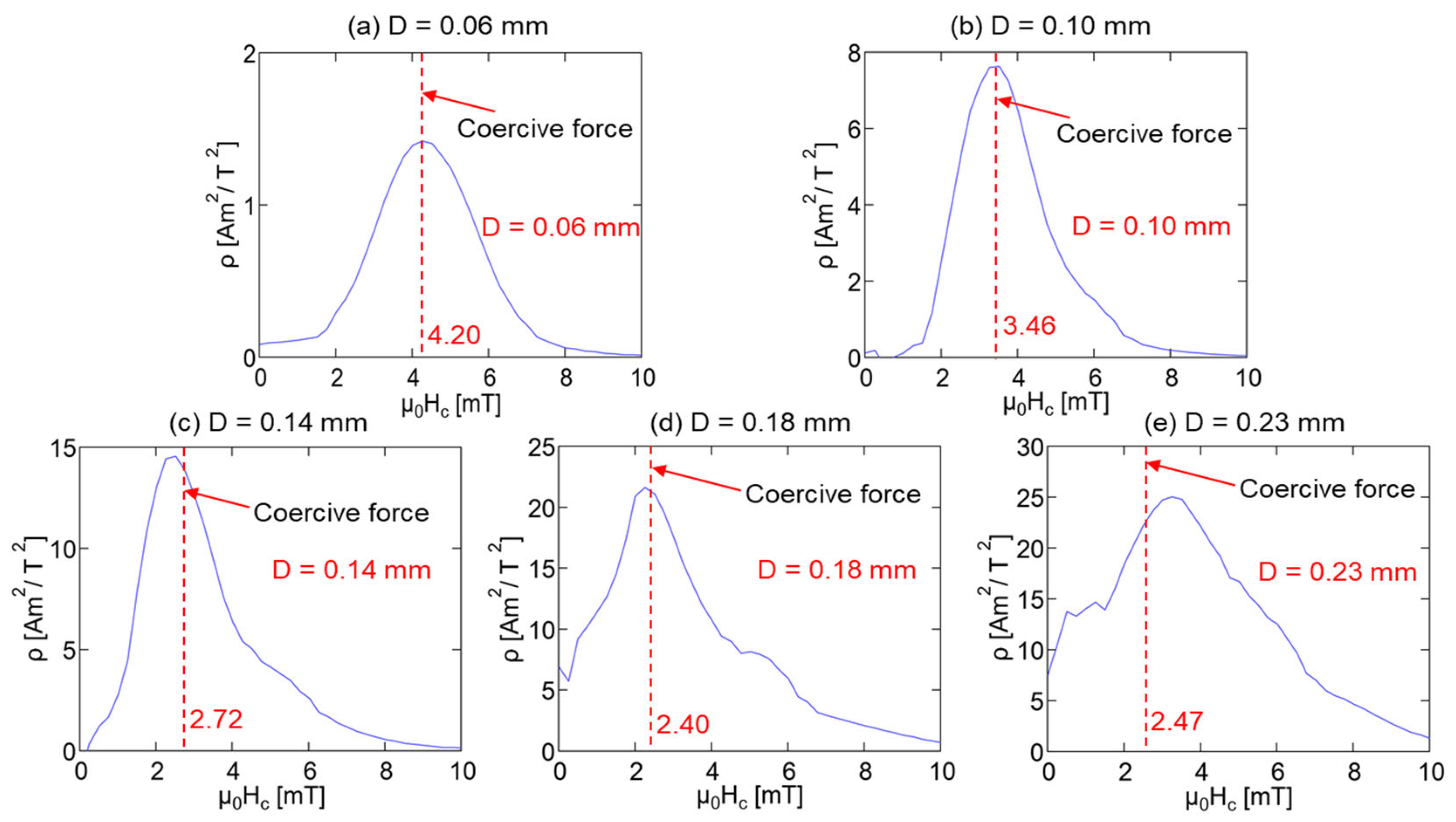
4.1. Correlation between Coercivity of Major Hysteresis Loop and FORC Distribution of Wiegand Wire
4.2. Single and Uniform Magnetic Structure
4.3. Three Layers of Magnetic Structure
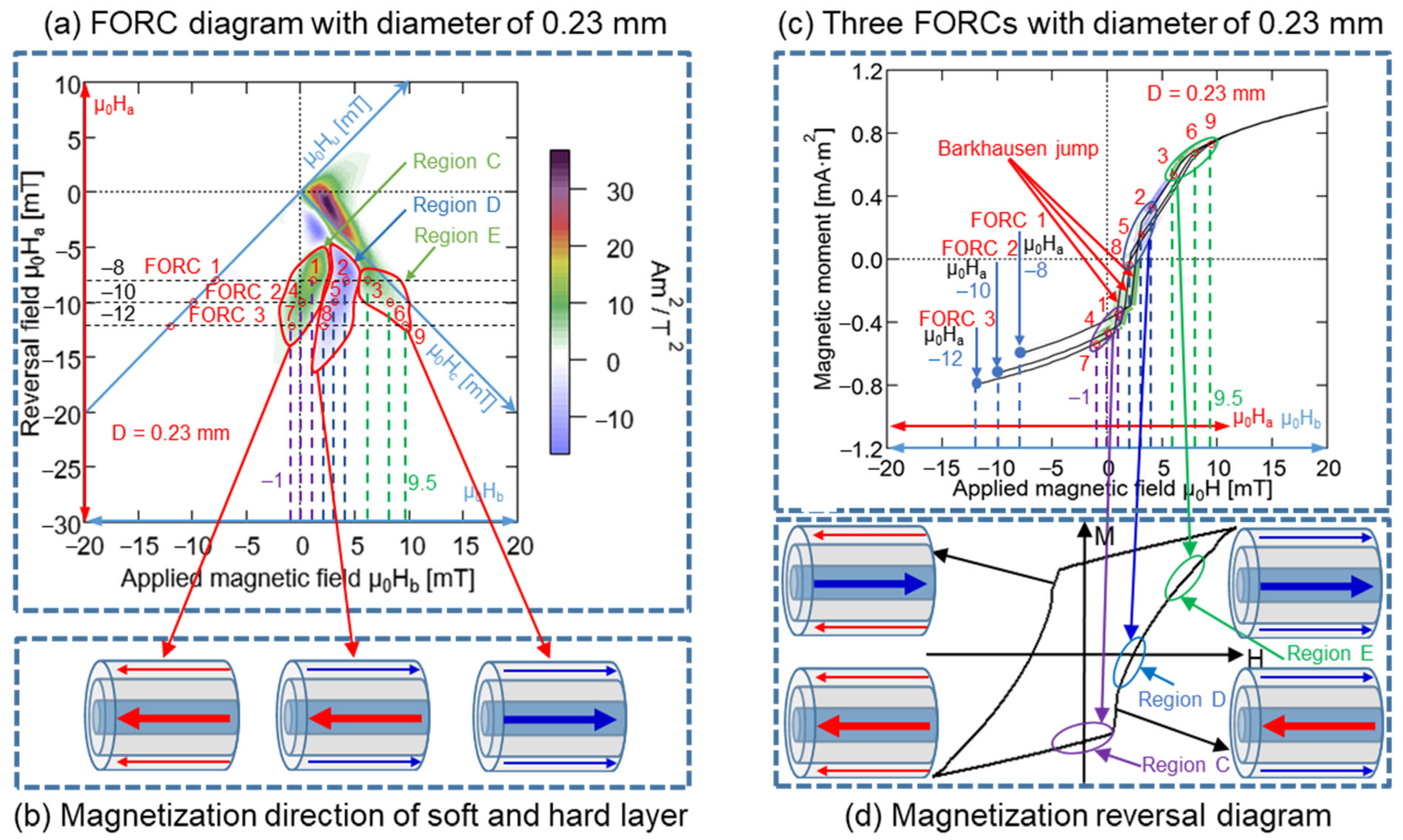
4.4. Relationship between Magnetization Reversal Direction of Wiegand Wire and Partial Region of FORC Distribution Diagram
5. Conclusions
Author Contributions
Funding
Institutional Review Board Statement
Informed Consent Statement
Data Availability Statement
Conflicts of Interest
References
- Wiegand, J.R.; Velinsky, M. Bistable Magnetic Device. U.S. Patent #3,820,090, 25 June 1974. [Google Scholar]
- Wiegand, J.R.; Velinsky, M. Method of manufacturing bistable magnetic device. U.S. Patent #3,892,118, 01 July 1975. [Google Scholar]
- Abe, S.; Matsushita, A. Induced pulse voltage in twisted Vicalloy wire with compound magnetic effect. IEEE Trans. Magn. 1995, 31, 3152–3154. [Google Scholar] [CrossRef]
- Yang, C.; Sakai, T.; Yamada, T.; Song, Z.; Takemura, Y. Improvement of pulse voltage generated by Wiegand sensor through magnetic-flux guidance. Sensors 2020, 20, 1408. [Google Scholar] [CrossRef] [PubMed] [Green Version]
- Inoue, A.; Masumoto, T.; Hagiwara, M.; Chen, H.S. The structural relaxation behavior of Pd48Ni32P20, Fe75Si10B15 and Co72.5Si12.5B15 amorphous alloy wire and ribbon. Scr. Metall. 1983, 17, 1205–1208. [Google Scholar] [CrossRef]
- Mohri, K.; Humphrey, F.B.; Kawashima, K.; Kimura, K.; Mizutani, M. Large Barkhausen and Matteucci effect in FeCoSiB, FeCrSiB, and FeNiSiB amorphous wires. IEEE Trans. Magn. 1990, 26, 1789–1791. [Google Scholar] [CrossRef]
- Makino, Y.; Costa, J.L.; Madurga, V.; Rao, K.V. Magneto-resistance stress effects and a self-similar expansion model for the magnetization process in amorphous wires. IEEE Trans. Magn. 1989, 25, 3620–3622. [Google Scholar] [CrossRef]
- Costa, J.L.; Makino, Y.; Rao, K.V. Effects of longitudinal currents and torsion on the magnetization processes in amorphous wires. IEEE Trans. Magn. 1990, 26, 1792–1794. [Google Scholar] [CrossRef]
- Rauscher, G.; Radeloff, C. Wiegand and Pulse-Wire Sensors. Sensors 1989, 5, 315. [Google Scholar]
- Serizawa, R.; Yamada, T.; Masuda, S.; Abe, S.; Kohno, S.; Kaneko, F.; Takemura, Y. Energy harvesting derived from magnetization reversal in FeCoV wire. In Proceedings of the IEEE Sensors, Taipei, Taiwan, 28–31 October 2012. [Google Scholar]
- Chen, Y.-H.; Lee, C.; Wang, Y.-J.; Chang, Y.-Y.; Chen, Y.-C. Energy Harvester Based on an Eccentric Pendulum and Wiegand Wires. Micromachines 2022, 13, 623. [Google Scholar] [CrossRef]
- Takemura, Y.; Fujiyama, N.; Takebuchi, A.; Yamada, T. Battery-less hall sensor operated by energy harvesting from a single Wiegand pulse. IEEE Trans. Magn. 2017, 53, 4002706. [Google Scholar] [CrossRef] [Green Version]
- Takahashi, K.; Takebuchi, A.; Yamada, T.; Takemura, Y. Power supply for medical implants by Wiegand pulse generated from a magnetic wire. J. Mag. Soc. Jpg. 2018, 42, 49–54. [Google Scholar] [CrossRef] [Green Version]
- Takahashi, K.; Yamada, T.; Takemura, Y. Circuit parameters of a receiver coil using a Wiegand sensor for wireless power transmission. Sensors 2019, 19, 2710. [Google Scholar] [CrossRef] [PubMed]
- Lien, H.-L.; Chang, J.-Y. Magnetic Reference Mark in a Linear Positioning System Generated by a Single Wiegand Pulse. Sensors 2022, 22, 3185. [Google Scholar] [CrossRef] [PubMed]
- Sun, X.; Yamada, T.; Takemura, Y. Output Characteristics and Circuit Modeling of Wiegand Sensor. Sensors 2019, 19, 2991. [Google Scholar] [CrossRef] [PubMed] [Green Version]
- Sun, X.; Iijima, H.; Saggini, S.; Takemura, Y. Self-Oscillating Boost Converter of Wiegand Pulse Voltage for Self-Powered Modules. Energies 2021, 14, 5373. [Google Scholar] [CrossRef]
- Felix, H.; Andreas, B. Direct Observation of Large Barkhausen Jump in Thin Vicalloy Wires. IEEE Magn. Lett. 2020, 11, 2506504. [Google Scholar]
- Kohara, T.; Yamada, T.; Abe, S.; Kohno, S.; Kaneko, F.; Takemura, Y. Effective excitation by single magnet in rotation sensor and domain wall displacement of FeCoV wire. J. Appl. Phys. 2011, 109, 07E531. [Google Scholar] [CrossRef] [Green Version]
- Yang, C.; Kita, Y.; Song, Z.; Takemura, Y. Magnetic Reversal in Wiegand Wires Evaluated by First-Order Reversal Curves. Materials 2021, 14, 3868. [Google Scholar] [CrossRef] [PubMed]
- Sha, G.; Yang, C.; Song, Z.; Takemura, Y. Magnetic Interaction in Wiegand Wires Evaluated by First-Order Reversal Curves. Materials 2022, 15, 5936. [Google Scholar] [CrossRef]
- Dlugos, D.J. Wiegand Effect Sensors Theory and Applications. Sensors 1998, 15, 32–34. [Google Scholar]
- Wiegand, J.R. Switchable Magnetic Device. U.S. Patent #3,560,278, 01 May 1978. [Google Scholar]
- Pike, C.; Fernandez, A. An investigation of magnetic reversal in submicron-scale Co dots using first order reversal curve diagrams. J. Appl. Phys. 1999, 85, 6668–6676. [Google Scholar] [CrossRef]
- Roberts, A.P.; Pike, C.R.; Verosub, K.L. First-Order Reversal Curve Diagrams: A New Tool for Characterizing the Magnetic Properties of Natural Samples. J. Geophys. Res. 2000, 105, 28461–28475. [Google Scholar] [CrossRef]
- Pan, Y.; Petersen, N.; Winklhofer, M. Rock magnetic properties of uncultured magnetotactic bacteria. Earth Planet. Sci. Lett. 2005, 237, 311–325. [Google Scholar] [CrossRef]
- Franco, V.; Gottschall, T.; Skokov, K.; Gutfleisch, O. First-Order Reversal Curve (FORC) Analysis of Magnetocaloric Heusler-Type Alloys. IEEE Magn. Lett. 2016, 7, 6602904. [Google Scholar] [CrossRef]
- Carvallo, C.; Muxworthy, A.R.; Dunlop, D.J. First-order reversal curve (FORC) diagrams of magnetic mixtures: Micromagnetic models and measurements. Phys. Earth Planet. Inter. 2006, 154, 3–4. [Google Scholar] [CrossRef]
- Harrison, R.J.; Feinberg, J.M. FORCinel: An Improved Algorithm for Calculating First-Order Reversal Curve Distributions Using Locally Weighted Regression Smoothing. Geochem. Geophys. Geosyst. 2008, 9, 5. [Google Scholar] [CrossRef]
- Dodrill, B.; Ohodnicki, P.; Leary, A.; McHenry, M. High-Temperature First-Order-Reversal-Curve (FORC) Study of Magnetic Nanoparticle Based Nanocomposite Materials. TechConnect Briefs 2016, 1, 45–48. [Google Scholar] [CrossRef]
- Shi, Z.X.; Zhou, D.Y.; Li, S.D.; Xu, J.; Uwe, S. First-order reversal curve diagram and its application in investigation of polarization switching behavior of HfO2 -based ferroelectric thin films. Acta Phys. Sin. 2021, 70, 127702. [Google Scholar] [CrossRef]
- Qin, H.F.; Liu, Q.S.; Pan, Y.X. The first-order reversal curve (FORC) diagram: Theory and case study. Chin. J. Geophys. 2008, 51, 743–751. (In Chinese) [Google Scholar]
- Muxworthy, A.R.; King, J.G.; Heslop, D. Assessing the ability of first-order reversal curve (FORC) diagrams to unravel complex magnetic signals. J. Geophys. Res. 2005, 110, B01105. [Google Scholar] [CrossRef]
- Heslop, D.; Muxworthy, A.R. Aspects of calculating first-order reversal curve distributions. J. Magn. Magn. Mater. 2005, 288, 155–167. [Google Scholar] [CrossRef] [Green Version]
- Pike, C.R.; Ross, C.A.; Scalettar, R.T.; Zimanyi, G. First-order reversal curve diagram analysis of a perpendicular nickel nanopillar array. Phys. Rev. B 2005, 71, 134407. [Google Scholar] [CrossRef] [Green Version]
- Acton, G.; Yin, Q.Z.; Verosub, K.L.; Jovane, L.; Roth, A.; Jacobsen, B.; Ebel, D.S. Micromagnetic coercivity distributions and interactions in chondrules with implications for paleointensities of the early solar system. J. Geophys. Res. Solid Earth 2007, 112, B03S90. [Google Scholar] [CrossRef]


| Region or Peak | D = 0.06 mm | D = 0.10 mm | D = 0.14 mm | D = 0.18 mm | D = 0.23 mm | Attribute | |||||
|---|---|---|---|---|---|---|---|---|---|---|---|
| μ0Hc (mT) | μ0Hu (mT) | μ0Hc (mT) | μ0Hu (mT) | μ0Hc (mT) | μ0Hu (mT) | μ0Hc (mT) | μ0Hu (mT) | μ0Hc (mT) | μ0Hu (mT) | ||
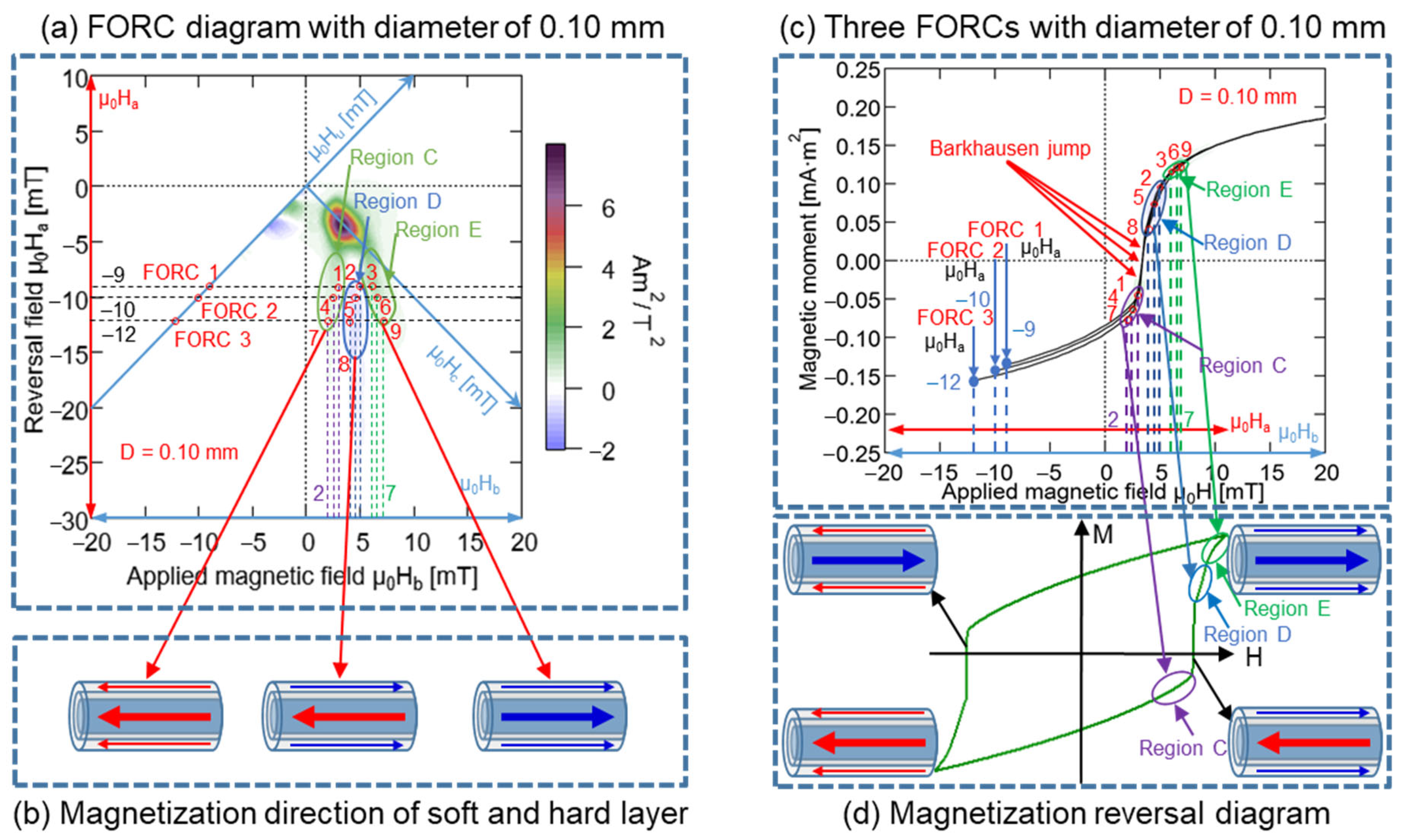
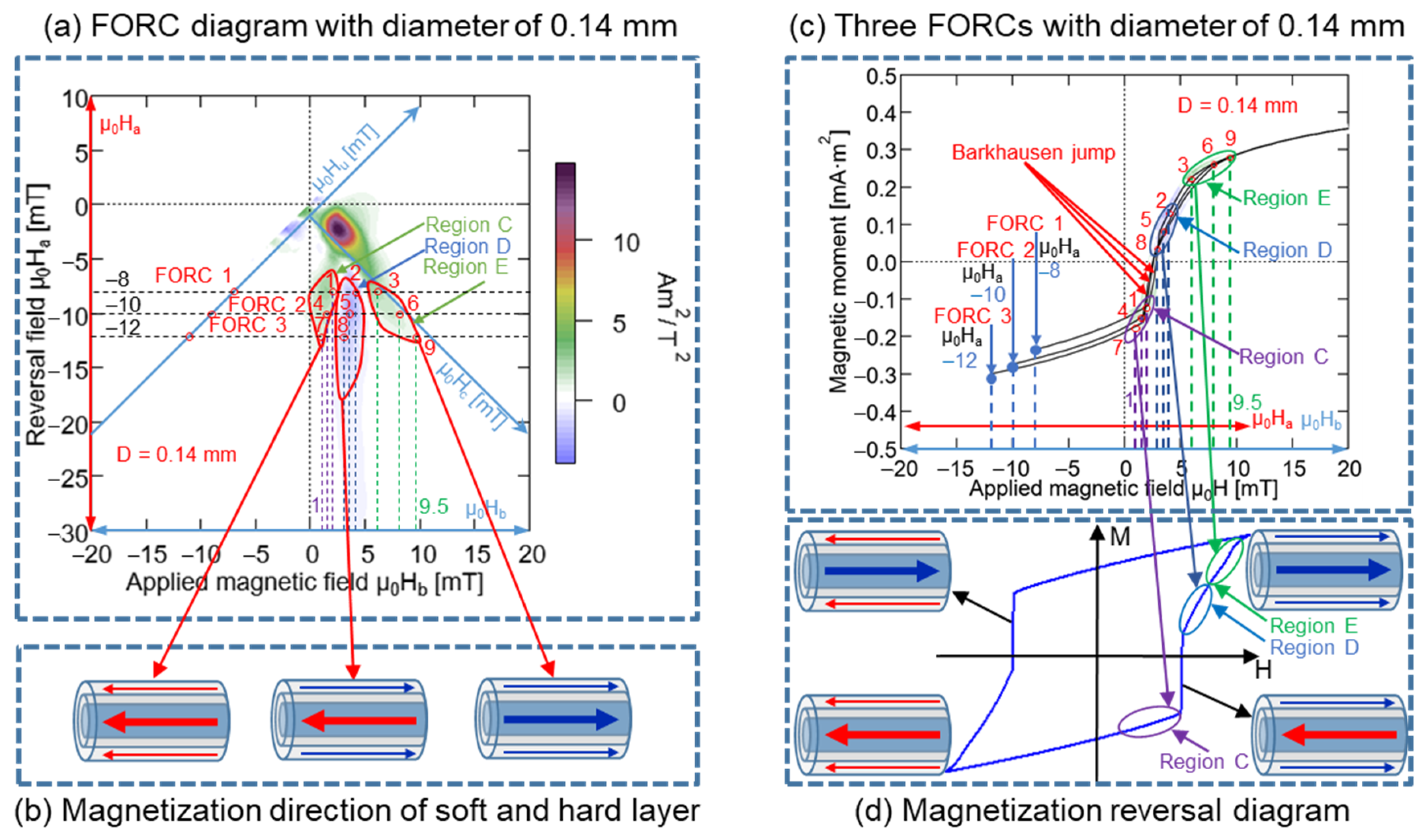
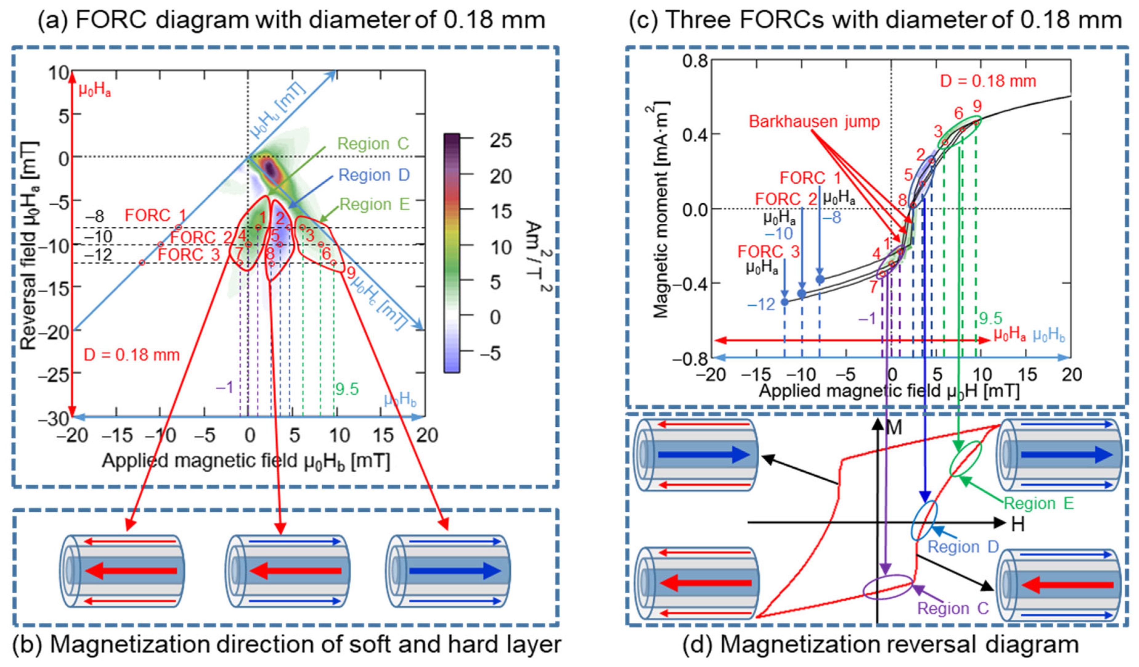
| Region A1 | \ | \ | 1.75–4.25 | −1.5 to 1.25 | 1.25–3.5 | −1 to 1.25 | 0.25–3.25 | −0.75 to 1.5 | 0–3.5 | −0.5 to 1.5 | Soft layer |
| Region A2 | \ | \ | 4.25–5.5 | −0.75 to 0.75 | 3.5–6.5 | −0.75 to 0 | 3.25–6.5 | −0.75 to 1.25 | 3.5–6.5 | −0.5 to 1.25 | Middle layer |
| Region B | \ | \ | \ | \ | \ | \ | 0.75–3 | −2.25 to −0.75 | 0.75–3.25 | −2 to −0.75 | Soft layer |
| Region C | \ | \ | 4.5–7.5 | −5.5 to −1.5 | 3.5–6.5 | −5.5 to −1.5 | 3.25–6.5 | −6.5 to −1.25 | 3.25–6.5 | −7.5 to −1.5 | Interaction |
| Region D | \ | \ | 6.5–10 | −5.5 to −2 | 4.5–9.75 | −6.75 to −1 | 4–8.25 | −5.75 to −1 | 4–9 | −7.5 to −1 | Interaction |
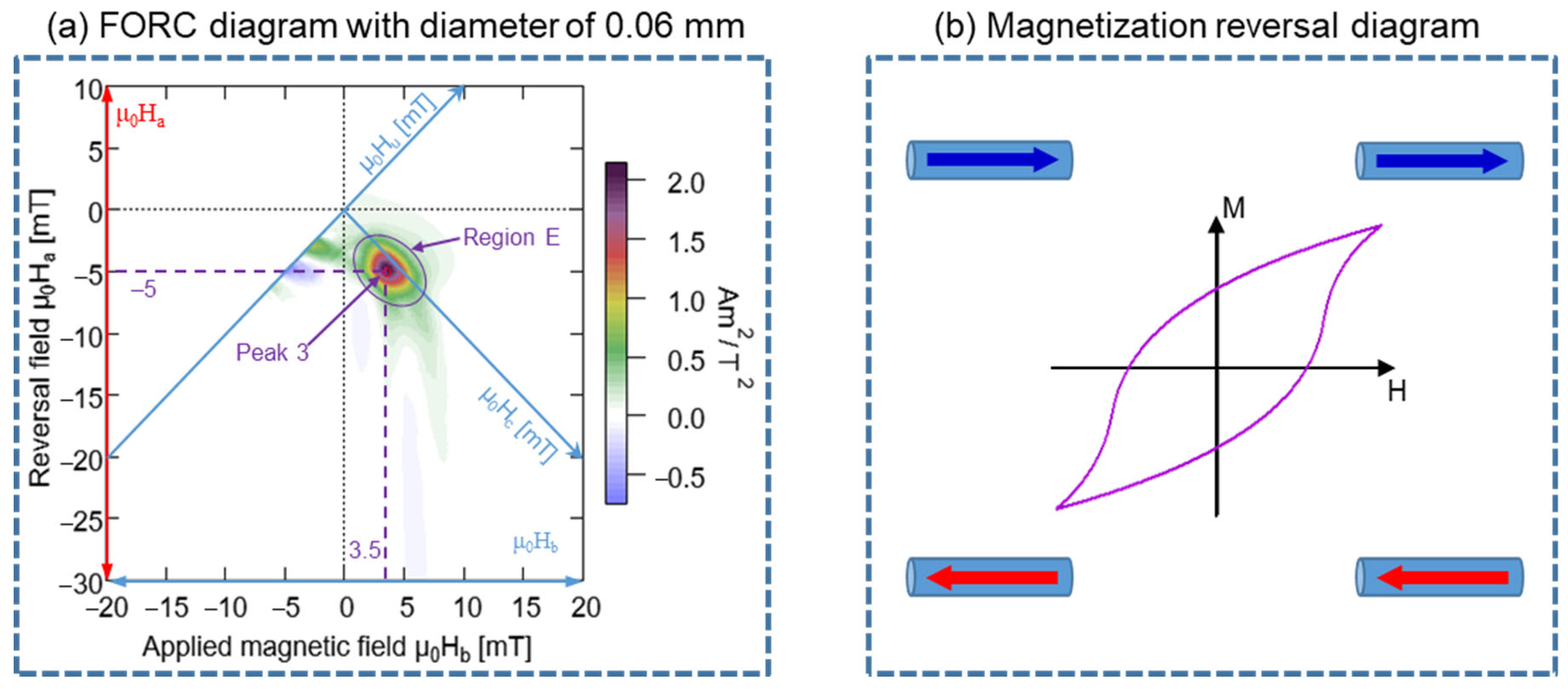
| Region E | 2.25–6.5 | −2 to 1.25 | 5.75–9.75 | −2.75 to 0.25 | 6.25–11.25 | −2.25 to −0.25 | 6.5–10.5 | −2 to 0.25 | 6.5–11.25 | −2 to 0.5 | Hard core |
| Region F | \ | \ | 2–5.5 | 1–3 | 1–3.75 | 1–3 | 0.25–3.5 | 1.5–4.75 | 0.25–2.5 | 1.25–5 | Interaction |
| Peak 1 | \ | \ | 3.5 | 0 | 2.75 | 0.25 | 2 | 0.5 | 1.75 | 0.75 | Soft layer |
| Peak 2 | \ | \ | 4.5 | 0 | 3.75 | −0.25 | 3.5 | 0 | 4.25 | 0.25 | Middle layer |
| Peak 3 | 4.25 | −0.75 | 7 | −1 | 7.5 | −1 | 7.75 | −0.75 | 8.25 | −0.75 | Hard core |
Publisher’s Note: MDPI stays neutral with regard to jurisdictional claims in published maps and institutional affiliations. |
© 2022 by the authors. Licensee MDPI, Basel, Switzerland. This article is an open access article distributed under the terms and conditions of the Creative Commons Attribution (CC BY) license (https://creativecommons.org/licenses/by/4.0/).
Share and Cite
Jiang, L.; Yang, C.; Song, Z.; Takemura, Y. Magnetic Structure of Wiegand Wire Analyzed by First-Order Reversal Curves. Materials 2022, 15, 6951. https://doi.org/10.3390/ma15196951
Jiang L, Yang C, Song Z, Takemura Y. Magnetic Structure of Wiegand Wire Analyzed by First-Order Reversal Curves. Materials. 2022; 15(19):6951. https://doi.org/10.3390/ma15196951
Chicago/Turabian StyleJiang, Liang, Chao Yang, Zenglu Song, and Yasushi Takemura. 2022. "Magnetic Structure of Wiegand Wire Analyzed by First-Order Reversal Curves" Materials 15, no. 19: 6951. https://doi.org/10.3390/ma15196951