Article

Computational Analysis of Fluid Forces on an Obstacle in a Channel Driven Cavity: Viscoplastic Material Based Characteristics

1
Department of Mathematics, Air University, PAF Complex E-9, Islamabad 44000, Pakistan
2
Department of Automation, Biomechanics and Mechatronics, Lodz University of Technology, 1/15 Stefanowskiego, St., 90-924 Lodz, Poland
3
Department of Mathematics, University of Management and Technology, Lahore 54770, Pakistan
4
Faculty of Materials and Manufacturing, College of Mechanical Engineering and Applied Electronics Technology, Beijing University of Technology, Beijing 100124, China
*
Author to whom correspondence should be addressed.
Materials 2022, 15(2), 529; https://doi.org/10.3390/ma15020529
Submission received: 7 November 2021 / Revised: 29 December 2021 / Accepted: 6 January 2022 / Published: 11 January 2022

Abstract

:
In the current work, an investigation has been carried out for the Bingham fluid flow in a channel-driven cavity with a square obstacle installed near the inlet. A square cavity is placed in a channel to accomplish the desired results. The flow has been induced using a fully developed parabolic velocity at the inlet and Neumann condition at the outlet, with zero no-slip conditions given to the other boundaries. Three computational grids, C1, C2, and C3, are created by altering the position of an obstacle of square shape in the channel. Fundamental conservation and rheological law for viscoplastic Bingham fluids are enforced in mathematical modeling. Due to the complexity of the representative equations, an effective computing strategy based on the finite element approach is used. At an extra-fine level, a hybrid computational grid is created; a very refined level is used to obtain results with higher accuracy. The solution has been approximated using P2P1 elements based on the shape functions of the second and first-order polynomial polynomials. The parametric variables are ornamented against graphical trends. In addition, velocity, pressure plots, and line graphs have been provided for a better physical understanding of the situation Furthermore, the hydrodynamic benchmark quantities such as pressure drop, drag, and lift coefficients are assessed in a tabular manner around the external surface of the obstacle. The research predicts the effects of Bingham number (Bn) on the drag and lift coefficients on all three grids C1, C2, and C3, showing that the drag has lower values on the obstacle in the C2 grid compared with C1 and C3 for all values of Bn. Plug zone dominates in the channel downstream of the obstacle with augmentation in Bn, limiting the shear zone in the vicinity of the obstacle.

1. Introduction

Even though the bulk of fluids in the biosphere exhibit Newtonian behavior, most synthetic and nonsynthetic industrial fluids, as well as biological fluids such as the blood, and saliva of humans, exhibit non-Newtonian behavior. Cosmetics, paints, soaps, glues, detergents, and various food items are a few examples. Among these, a substantial class of non-Newtonian materials known as viscoplastic materials or Bingham plastic has a yield stress limit that must be accomplished before considerable deformation can occur. This type of non-Newtonian substance is very important. The viscoplastic fluids include slurries and chocolate, pastes and margarine, mayonnaise, suspension, and others. These ingredients have been used in many sectors and culinary processes and are currently an area of increased scientific interest because of their excellent functionality, practical use, and wide-ranging applicability.
The initial idea of yield stress and its technical aspects was communicated by Shwedov [1], who assessed the behavior of flow, composition, and the quality of viscoplastic materials at various output stress levels. Following Shwedov, an extensive range of experiments was conducted by Bingham, who carried out detailed observations of their fluidity and plasticity [2]. Since then, the interest in these materials has been growing steadily, resulting in numerous studies, modeling, and simulations, that examine such materials in nontrivial flows, either conceptually or experimentally. Several models have such as the Bingham [2], the Herschel–Bulkley [3], and the Casson model [4], attempted to show the relationship between stress and strain in these fluids and gain a better understanding of the physical properties of viscoplastic materials. Thus far, Bingham fluid model seems the strongest; Bingham accomplished remarkable feats by proposing many viscoplastic paints and clarifying the plasticity and fluidity of these materials. Subsequently, Bird et al. [5,6] undertook seminal research, providing a list of several additional materials that exhibit these features. Several attempts [7,8,9] have been made to amend Bingham’s modeling of plastic fluids and create mathematical solutions. Bercovier and Engelmann [7] recognized the discontinuity found in the Bingham model and provided the corrective by linearizing the fluid viscosity. Papanastasiou [8] added to the expression of yield stress by introducing an exponential term. This addition to the model aids in describing yielded and unyielded areas. Barnes [9] provided a detailed study of fluid viscoplastic behavior, stating that the behavior of real viscoplastic fluids is more similar to the Papanastasiou’s regularized viscoplastic fluid than the behavior of ideal Bingham fluid. Further research on yield-stress fluids can be found in [10,11,12,13,14,15].
Much research has been dedicated to the theoretical and practical aspects of the channel flow using Bingham fluids. For the system overriding the motion, the weak solutions have been addressed in [16], and in pipes and plane channel Poiseuille flow, nonlinear stability has been investigated in [17]. For the problem of incoming flow in a pipe, spatial decay estimations have been studied in [18], and slip conditions are used to study Couette–Poiseuille flow in a porous channel in [19]. The convective flow of Bingham fluid in a vertical channel has also been studied; for the Couette–Poiseuille flow, the natural convection is studied in [20]. In a porous channel, the influence of exterior and internal heating on the free convective flow has been explored using Pascal’s piecewise-linear law for Poiseuille flow in [21] and in [22] for mixed convection of non-Newtonian fluids, the analytic solutions have been produced.
The flow around obstacles is a fascinating fluid mechanics problem from a computational, experimental, and analytical standpoint. Due to technological developments in recent years, difficulties with the computational and temporal issues associated with simulations around obstacles have been eliminated. Researchers nowadays focus their efforts on gaining a better knowledge of fluid movement around obstacles and interpreting it physically. Schaefer et al. [23] carried out ground-breaking work in this area by studying the flow characteristics of Newtonian fluid flow around an obstacle. Outcomes for Newtonian fluid throughout the cylinder accompanied by different physical necessities can be found in [24,25,26,27]. The literature includes limited work on non-Newtonian fluids flowing around obstacles. C. H. K. Williamson [24] investigated the characteristics of vortex shedding over a bluff body. Hussain et al. [25] considered continuous and discontinuous Galerkin approaches for computing incompressible problems and investigated the control of the mean flux. Kanaris et al. [26] studied the features of the 3D flow field over an obstacle in a channel and analyzed the confinement only in far wake. Rajani et al. [27] have focused on describing the viscous flow over a cylinder in a channel. The main findings are validated against skin friction and Strouhal frequency shedding. Adachi and Yoshioka [28] investigated the theoretical work in this area. Tokpavi et al. [29,30] examined Bingham fluids around the circular cylinder, including inertia effects. They examined the flow characteristics of Bingham fluid experimentally and showed excellent agreement between earlier theoretical conclusions and their experimental data. The Bingham fluid was exploited by Nirmalkar et al. [31] to explain the forced thermal convection effect past a square shape cylinder. The drag and lift coefficients magnitudes were determined for Reynolds number (Re) = 45 by Mossaz et al. [32] and Syrakos et al. [33] for different values of Bingham number. Moreover, Syrakos et al. [34] investigated the idea of an effective Reynolds number for Bingham fluid.
Abbasi et al. [35] quantitatively evaluated the effects of fluid forces using a cylinder-based Lattice Boltz–Mann Method (LBM) at low Reynolds numbers. Using P 2 P 1 element pair for finite element approach to a channel-driven cavity, Mahmood et al. [36] examined the non-Newtonian flow. Khan et al. [37] used the COMSOL solver to impose least-square FEM computation of viscous fluid flow through a semicylinder block. To tackle a flow problem, Tomio et al. [38] constructed a numerical approach, second-order, finite difference schemes. Recently, Afraz et al. [39] provided a full investigation of fluid forces and thermal analysis of two-dimensional, incompressible, and laminar complicated fluid flow.
The flow of Bingham material has been investigated by many researchers both computationally and experimentally. However, Bingham flow in the present configuration in the presence of obstacles is new. The discussion below is organized as follows; in Section 2, mathematical modeling is explained. The physical configuration and numerical approach are executed in Section 3. A detailed analysis of results is considered in Section 4, and the conclusion is offered in Section 5.

2. Mathematical Modeling

In dimensional form, the model Equations for steady, incompressible flows are defined in [15] as follows:
. u = 0
ρ ( u . u ) = p + . τ
where all the symbols have their traditional meanings. Bingham [2] developed a basic rheological relationship for viscoplastic materials:
{         γ ˙ = 0 ,                                       τ τ y τ = ( τ y γ ˙ + μ P ) ,     τ > τ y  
where the τ ,   γ ˙ ,   τ y   and   μ P denotes the stress tensor, the rate of the strain tensor, the yield stress, and plastic viscosity, respectively. The strain tensor is defined as
γ ˙ u + ( u ) T
Here, u denotes the velocity vector. Defining stress magnitude and strain rate as
τ [ 1 2 ( τ ) : ( τ ) ] 1 2 ,         γ ˙ . [ 1 2 ( γ ˙ ) : ( γ ˙ ) ] 1 2
One crucial observation is that the computational domain can be divided into three areas for viscoplastic fluids, the first where γ ˙ 0 defines the shear zone, whereas γ ˙ 0 shows plug zone and U 0 . There is a discontinuity inherited by Equation (3) which is addressed by Papanastasiou [8] using exponential function as
τ = [ τ y γ ˙ { 1 e x p ( m γ ˙ ) } + μ P ] γ ˙
Here, the parameter m denotes the stress growth. The viscosity, by owing Equation (4), can be written as
η = [ τ y γ ˙ { 1 e x p ( m γ ˙ ) } + μ P ]
Which for the entire flow domain is valid.
Introducing, u * , τ * , γ ˙ *   and   p * the nondimensional variables and choosing L r e f and U r e f as reference length and velocity, respectively, such that
. u * = 0
R e   u * . u * = p * + . τ *
In which
τ * = [ τ y γ ˙ * { 1 e x p ( M γ ˙ * ) } + 1 ] γ ˙ *
where R e = ρ U r e f L r e f μ P is Reynolds number and Bingham number is B n = τ y L r e f μ P U r e f . The parameter m is now given by M = m U r e f L r e f . The nondimensional form of viscosity is
η * = [ B n γ ˙ * { 1 e x p ( M γ ˙ * ) } + 1 ]
M is the nondimensional correspondence of m.
The hydrodynamic forces are accessible, the drag coefficient and lift coefficient C D and C L are immediately available for postprocessing by a nondimensional analog
C D = 2 F d ρ U m e a n 2 D
C L = 2 F l ρ U m e a n 2 D
Here, U m e a n denotes reference velocity, and D is the diameter of the obstacle.

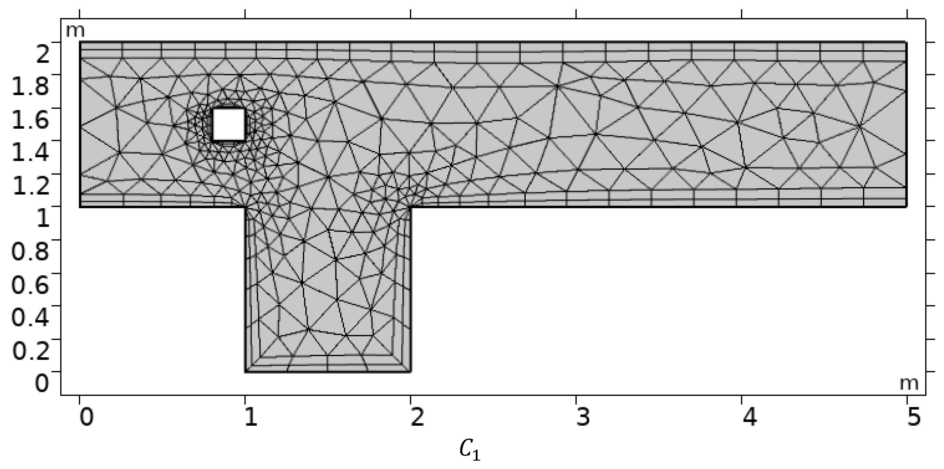
3. Physical Configuration and Numerical Scheme

A schematic diagram of the channel-driven cavity is shown in Figure 1. An open square cavity is placed at the bottom of the channel. A parabolic inflow profile is provided at the channel’s inlet, and at the outlet, a Neumann condition is addressed. The other walls of the channel-driven cavity is set zero no-slip condition, i.e., u = v = 0 . For more accuracy of hydrodynamic forces, an extra-fine hybrid mesh is developed around the obstacles. A square shape cylinder is placed by varying the locations with centers respectively, (0.9, 1.5), (1.5, 1.5), and (2.1, 1.5).
Considering incompressible Navier–Stokes equations given in (1) and (2), together with the rheological law (3) representing Bingham material, a broad range of flow problems can be described. These equations describe the natural processes of life and contribute to understanding the flow of materials in nature. Due to the high nonlinearity of the model, exact solutions to such problems are rare; therefore, we apply FEM computation for the numerical approximation of the governing equations. In this direction, the conforming element pair 2 1 is selected for the velocity and pressure approximations. This element is a stable pair satisfying the inf–sup condition [40,41,42,43]. Newton’s method is applied to solve discrete nonlinear algebraic systems, and the inner linear subproblems are solved using a direct solver. The nonlinear iteration’s convergence condition is specified as follows:
| X n + 1 X n X n + 1 | < 10 6
where X denotes the general component of the solution.
The coarse computational grid for three different obstacle settings C 1 , C 2 , and C 3 are shown in Figure 2. Mesh refinement is an important step in validating any finite element model and enhancing the reader’s trust in the work’s physical outcomes. Since the finite element method (FEM) is based on a transformation of computational domain into the finite number of elements, in Table 1, mesh statistics at different refinement levels for several elements (# EL), and associated degrees of freedom (# DOF) are enumerated.

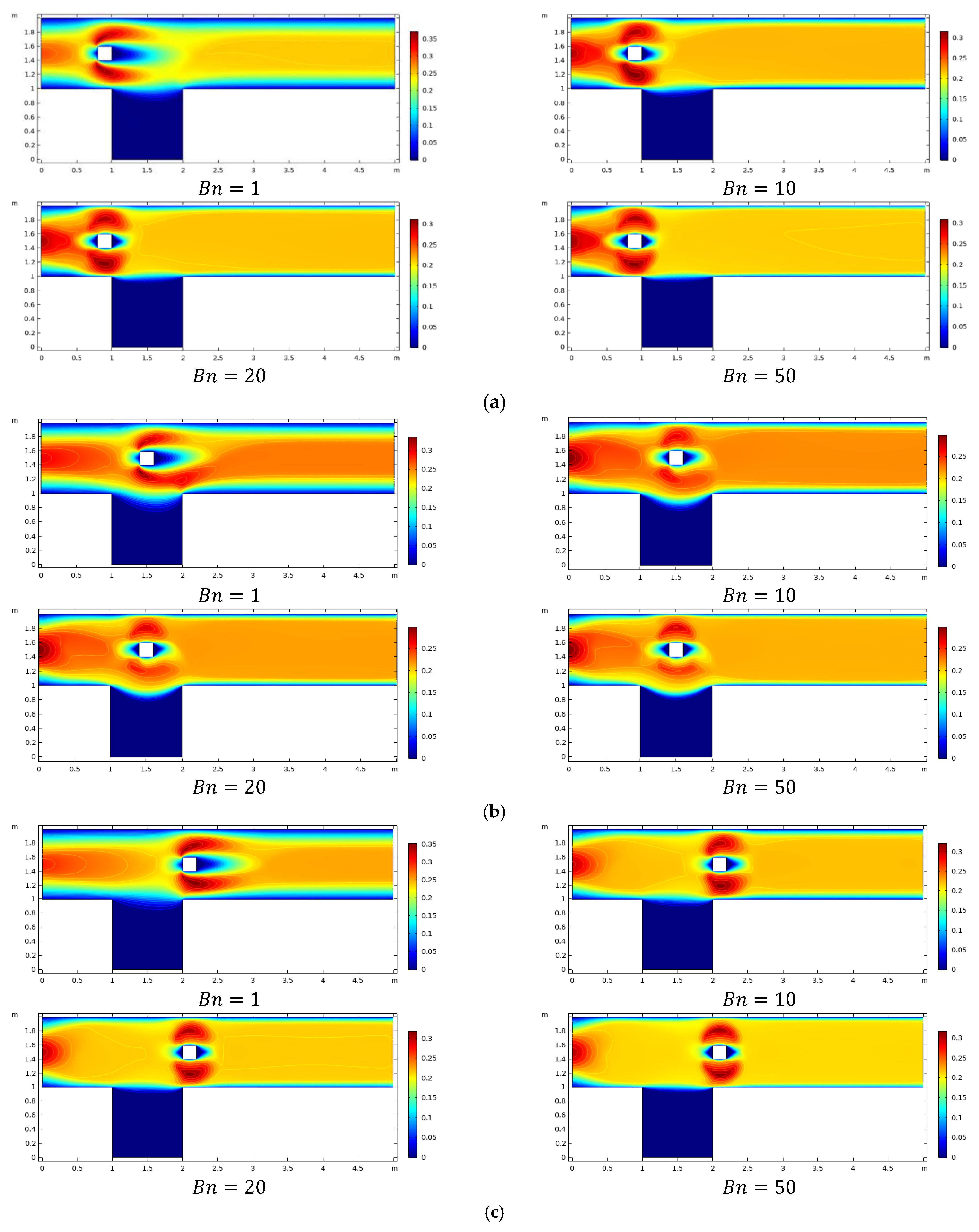
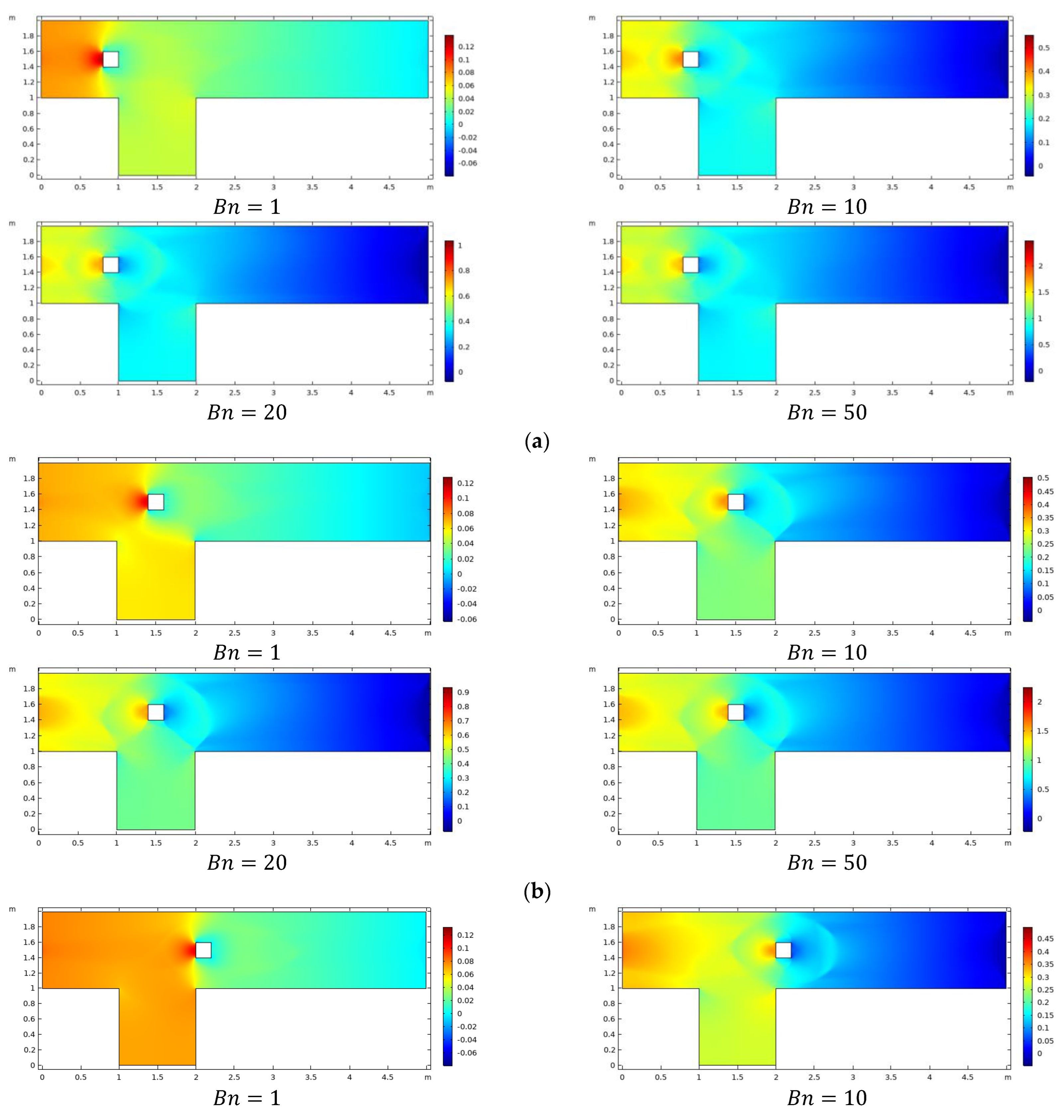
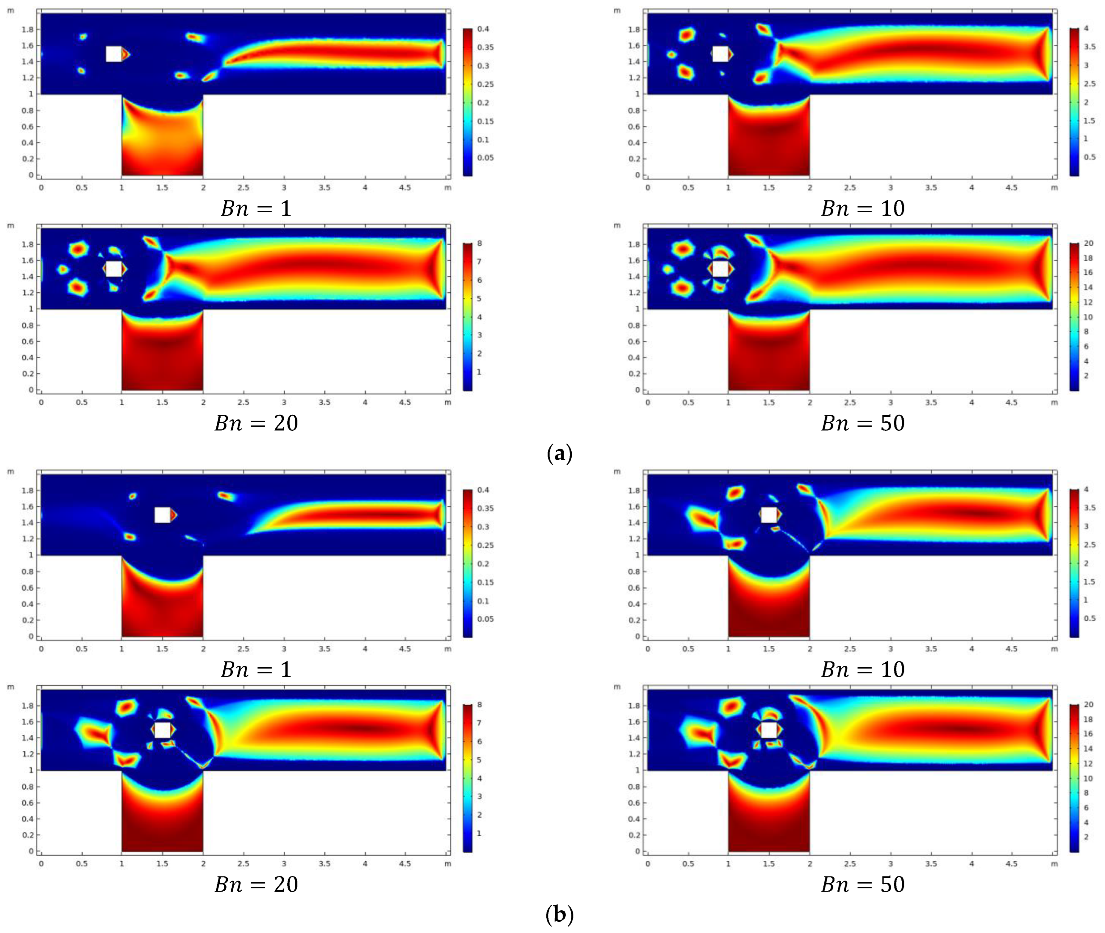
4. Results and Discussions

Figure 3a–c illuminates momentum distribution by adjusting Bingham number from B n = 1 up to 50. The position of the square obstacle is changed, centered at different C 1 , C 2 , and C 3 . The Bingham fluid flow is seen at a fixed Reynolds number R e = 20 . Fluctuation in velocity near an obstacle and other regions of the channel-driven cavity is noticed because the induced velocity at the inlet is parabolic, while for other boundaries, there is a no-slip condition. For all locations C 1 , C 2 , and C 3 , it is observed that velocity decreases with an increase in B n , and the plug zone stretches from the channel’s center to the solid walls, while the shear zone is limited to the immediate vicinity of obstacles.
The pressure changes across the physical domain, particularly in the presence of obstacles located at three different sites by varying B n , for restricted value R e = 20 , is plotted in Figure 4a–c. The figure illustrates that pressure behaves nonlinearly near the obstacle before becoming linear downstream, as predicted in channel flow. Because of plasticity effects amplified by enhancement in the value of B n , the parabolic profile given at the inlet quickly bifurcates at the obstacle and subsequently decreases in the center of the channel. The maximum value of optimal pressure is observed in the presence of an obstacle that interacts with the fluid.
The influence of relevant parameters on viscosity is plotted in Figure 5a–c. By increasing the magnitude of B n , an increase in viscosity is also observed. Higher viscosity values are seen as B n increases even for different obstacle positions. In addition, around the obstacle, there are small islands of high viscosity for all obstacle sites, and their size is growing with increasing B n .
Figure 6a–c depicts line graphs expressing velocity variations at various points in the physical configuration. Because viscosity does not affect injected velocity, a perfect parabolic peak is achieved at the inlet, as seen in the above illustrations. The fluid flow through the channel, on the other hand, varies its behavior near the obstacle and above the cavity. A gradual rise in nonlinearity can also be detected due to B n growth.
For increasing values of Bingham number ( B n ) and confining R e = 20 , Table 2 interprets fluctuation in the pressure across obstacles placed at distinct points in the channel, such as the centers at C 1 , C 2 , and C 3 . It is enumerated from the numerical data obtained by increasing B n pressure drop. The viscosity of Bingham fluids increases as B n increases, causing it to contact the obstacle with greater force and thereby increasing pressure drop. The numeric data obtained for B n ranging from (1 to 50) indicates that the pressure gradient approaches 1.144143 at the obstacle’s position G 1 and approaches 1.129823 and 1.164679 at the obstacle’s positions C 2 and C 3 , respectively. It is also observed that the obstacle’s position affects the pressure gradient. The manipulated difference is evidenced by tabulated values at B n = 1 for restriction R e = 20 , for location C 1 of the obstacle, the pressure drop value is 0.105098, whereas for the same value of B n and R e at the other two locations, i.e., at C 2 = 0.089917 and C 3 = 0.102492 variation in the pressure drop is observed. These findings show that the maximum pressure near the inlet pressure falls over the cavity pressure drops with low intensity, followed by the elevation after the fluid crosses from the cavity.
Table 3 depicts changes in benchmark hydrodynamic parameters such as drag coefficient and lift coefficient on the exterior surface of the obstacle located at C 1 , C 2 and C 3 . It is found that increasing the scale of B n drag and lift, coefficients fluctuate for a fixed value of Reynold number R e = 20 . The negative lift coefficient ( C L ) value illustrates that the lift forces are dominant in the upward direction. The cause for the negative value of lift coefficient is because the obstacle is positioned as if fluid enters the cavity and pushes the obstacle upward, resulting in a numerical pattern like this. From calculated values of drag coefficient at C 1 , C 2 , and C 3 , it is realized that the maximum value of drag is 6.511467 6 at C 1 . By fixing B n = 1 and R e = 20 as it comes closer to C 2 , drag value starts to decrease, having a magnitude of 5.71877 and again increases at C 3 as the magnitude is 6.615889 6. The lift coefficient’s contrasting behavior is adjusted so that fluctuation occurs at C 1 , C 2 , and C 3 as the magnitude of lift coefficient at C 1 = 0.24909 , at the location C 2 decreased value is noticed of magnitude −0.37351 and again increased to 0.28946 at C 3 . Because upward lift forces dominate, negative values are measured when the obstacle is positioned near the inlet and above the cavity position, while positive values are measured at C 3 because lift forces are active from downward.

5. Conclusions

The current study investigates the flow characteristics of a generalized Bingham material flow in a channel-driven cavity, with an obstacle of square shape positioned at various locations inside the channel. The physical problem and relevant rheological laws are transformed into a mathematical form using the Navier–Stokes equation in two-dimension and boundary constraints. The finite element method, a well-known computational tool, is required to report both the solution and the physical occurrences. Graphical trends are used to present the results. The behavior of the momentum distribution of a Bingham fluid at entrance, obstacle, and close to exit regions is represented by bar lines. The pressure variation, as well as the drag coefficient and lift coefficient on the external surface of the obstacle, are tabulated. The most important findings are listed below.
  • As the Bn increases, pressure drops become more vigorous for all obstacle positions.
  • The pressure drop is influenced by the placement of the obstacle, which increases at C1, lowers at C2, and finally boosts at C3.
  • Lift coefficient changes sign-on C2 when Bn exceeds the value Bn = 10 while on other grids, sign change does not occur.
  • Negative lift coefficients are obtained when upward forces dominate, while positive values are obtained when downward forces dominate.
  • Pressure has stagnant values at the front of the obstacle where fluid is interacting with it.
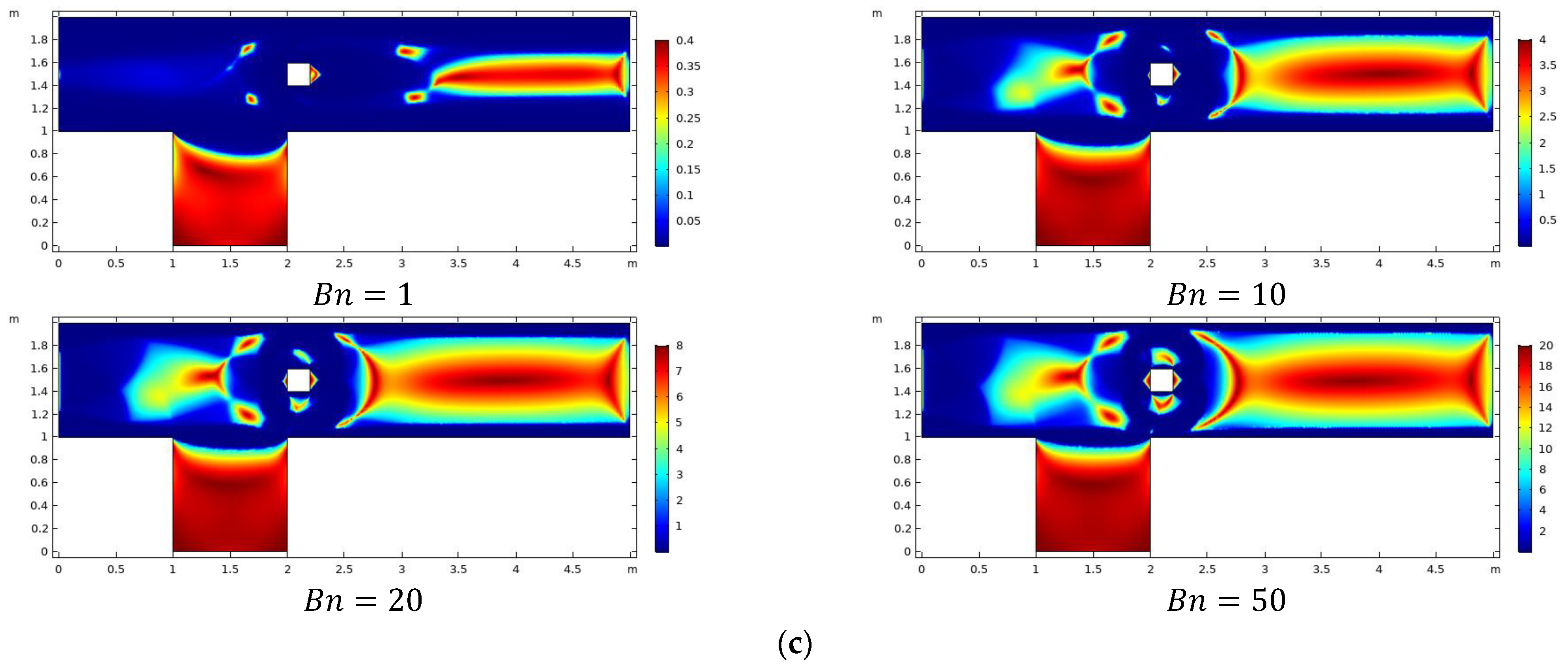
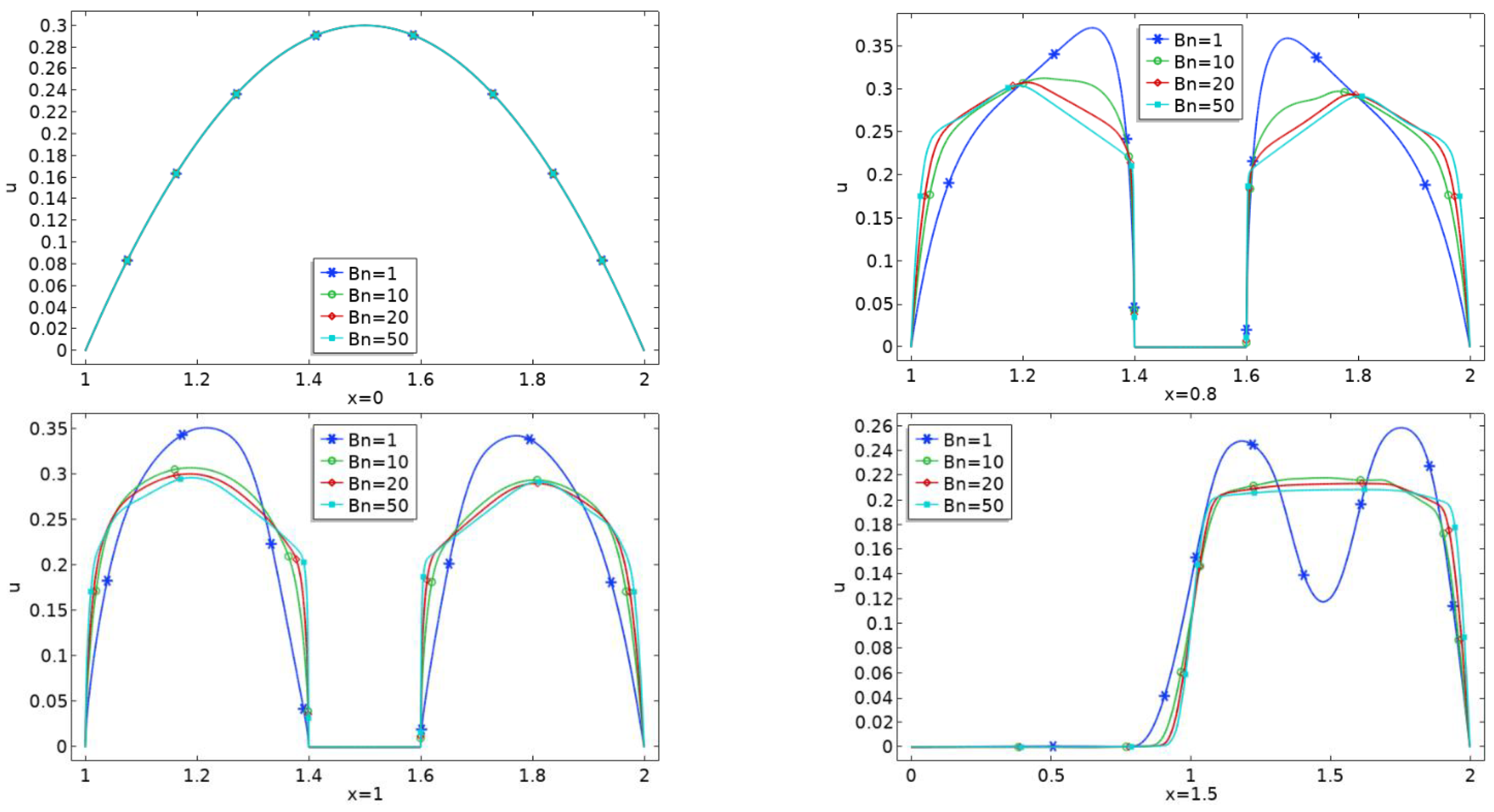
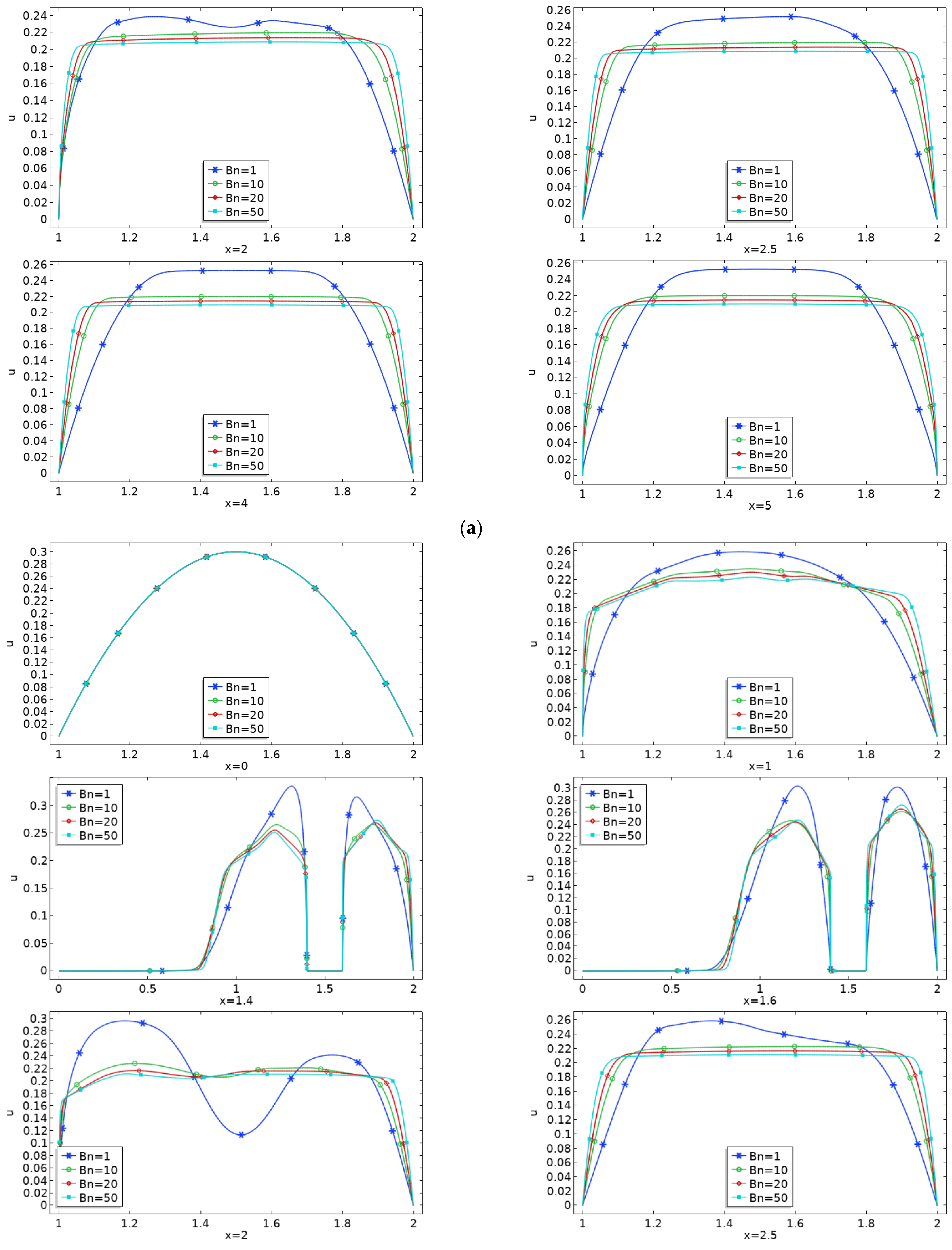
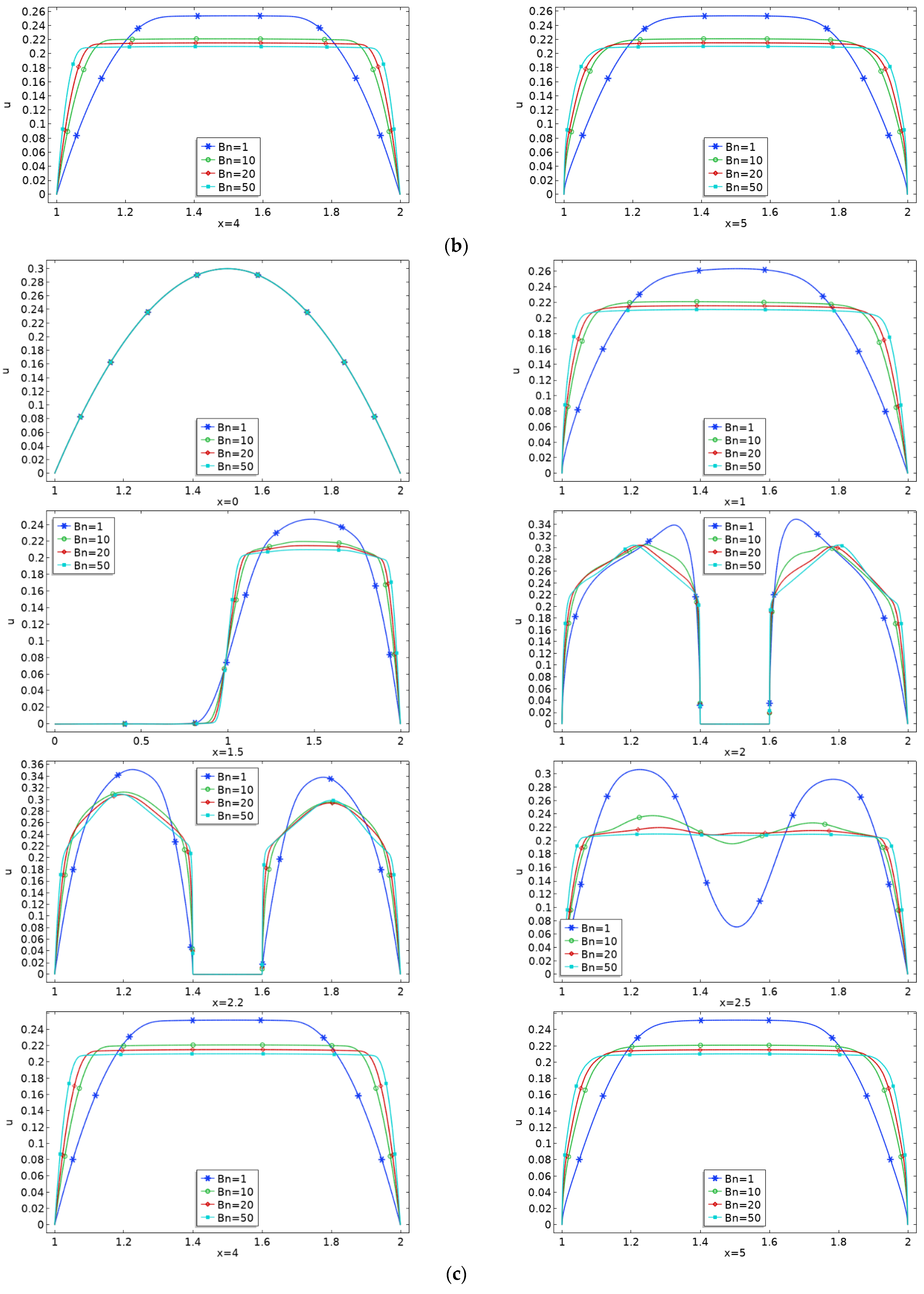
  • Plug zone enhances in the channel downstream of the obstacle with augmentation in Bn limiting the shear zone in the vicinity of the obstacle.

Author Contributions

Conceptualization, R.M.; methodology, A.H.M. and Q.u.A.; software, A.H.M.; validation, H.S.; formal analysis, I.S.; writing—original draft preparation, A.H.M. and Q.u.A.; writing—review and editing, A.H.M. and J.A.; visualization, R.M.; supervision, R.M.; funding acquisition, J.A. All authors have read and agreed to the published version of the manuscript.

Funding

This research received no external funding.

Institutional Review Board Statement

Not applicable.

Informed Consent Statement

Not applicable.

Data Availability Statement

Data is available on request from the corresponding author.

Conflicts of Interest

The authors declare no conflict of interest.

Nomenclature

τ y Yield Stress
μ p Plastic Viscosity
τ Stress Tensor
γ ˙ Rate of Strain Tensor
u Dimensional Velocity Vector
u * Dimensionless Velocity Vector
U i n Velocity at inlet
U m e a n Average Velocity
γ ˙ Shear Rate
p Dimensional pressure
p * Dimensionless pressure
m Dimensional Stress growth parameter
MDimensionless Stress growth parameter
R e Reynold number
B n Bingham number
# ELNumber of Elements
# DOFNumber of degrees of freedom
C D Drag Coefficient
C L Lift Coefficient

References

  1. Shwedov, F.N. La Rigidite de liquids. Rapp. Congr. Intern. Phys. Paris 1900, 1, 478–483. [Google Scholar]
  2. Bingham, E.C. Fluidity and Plasticity; McGraw-Hill: New York, NY, USA, 1922; Volume 2. [Google Scholar]
  3. Herschel, W.H.; Bulkley, R. Konsistenzmessungen von Gummi-Benzollösungen. Colloid Polym. Sci. 1926, 39, 291–300. [Google Scholar] [CrossRef]
  4. Casson, N. A Flow Equation for Pigment-Oil Suspensions of the Printing Ink type. Rheol. Disperse Syst. 1959, 3, 84–104. [Google Scholar]
  5. Bird, R.B.; Dai, G.; Yarusso, B.J. The Rheology and Flow of Viscoplastic Materials. Rev. Chem. Eng. 1983, 1, 1–70. [Google Scholar] [CrossRef]
  6. Bird, R.B.; Armstrong, R.C.; Hassager, O. Fluid Mechanics. In Dynamics of Polymeric Liquids, 2nd ed.; John Wiley and Sons Inc.: New York, NY, USA, 1987; Volume 1, p. 784. [Google Scholar]
  7. Bercovier, M.; Engelman, M. A finite-element method for incompressible non-Newtonian flows. J. Comput. Phys. 1980, 36, 313–326. [Google Scholar] [CrossRef]
  8. Papanastasiou, T.C. Flows of Materials with Yield. J. Rheol. 1987, 31, 385–404. [Google Scholar] [CrossRef]
  9. Barnes, H.A. The yield stress—A review—Everything flows? J. Nonnewton. Fluid Mech. 1999, 81, 133–178. [Google Scholar] [CrossRef]
  10. Syrakos, A.; Georgiou, G.C.; Alexandrou, A.N. Solution of the square lid-driven cavity flow of a Bingham plastic using the finite volume method. J. Non-Newton. Fluid Mech. 2013, 195, 19–31. [Google Scholar] [CrossRef] [Green Version]
  11. Mitsoulis, E.; Zisis, T. Flow of Bingham plastics in a lid-driven square cavity. J. Non-Newton. Fluid Mech. 2001, 101, 173–180. [Google Scholar] [CrossRef]
  12. Dean, E.J.; Glowinski, R.; Guidoboni, G. On the numerical simulation of Bingham visco-plastic flow: Old and new results. J. Non-Newton. Fluid Mech. 2007, 142, 36–62. [Google Scholar] [CrossRef]
  13. Kefayati, G.; Huilgol, R. Lattice Boltzmann method for the simulation of the steady flow of a Bingham fluid in a pipe of square cross-section. Eur. J. Mech.-B/Fluids 2017, 65, 412–422. [Google Scholar] [CrossRef]
  14. Kefayati, G. FDLBM simulation of magnetic field effect on non-Newtonian blood flow in a cavity driven by the motion of two facing lids. Powder Technol. 2014, 253, 325–337. [Google Scholar] [CrossRef]
  15. Mahmood, R.; Kousar, N.; Yaqub, M.; Jabeen, K. Numerical Simulations of the Square Lid Driven Cavity Flow of Bingham Fluids Using Nonconforming Finite Elements Coupled with a Direct Solver. Adv. Math. Phys. 2017, 2017, 1–10. [Google Scholar] [CrossRef]
  16. Obando, B.; Takahashi, T. Existence of weak solutions for a Bingham fluid-rigid body system. Ann. De L’institut Henri Poincaré C Anal. Non Linéaire 2018, 36, 1281–1309. [Google Scholar] [CrossRef] [Green Version]
  17. Nouar, C.; Frigaard, I. Nonlinear stability of Poiseuille flow of a Bingham fluid: Theoretical results and comparison with phenomenological criteria. J. Non-Newton. Fluid Mech. 2001, 100, 127–149. [Google Scholar] [CrossRef]
  18. Borrelli, A.; Patria, M.C.; Piras, E. Spatial decay estimates in the problem of entry flow for a Bingham fluid filling a pipe. Math. Comput. Model. 2004, 40, 23–42. [Google Scholar] [CrossRef]
  19. Chen, Y.-L.; Zhu, K.-Q. Couette–Poiseuille flow of Bingham fluids between two porous parallel plates with slip conditions. J. Non-Newton. Fluid Mech. 2008, 153, 1–11. [Google Scholar] [CrossRef]
  20. Barletta, A.; Magyari, E. Buoyant Couette–Bingham flow between vertical parallel plates. Int. J. Therm. Sci. 2008, 47, 811–819. [Google Scholar] [CrossRef]
  21. Rees, D.A.S.; Bassom, A.P. The Effect of Internal and External Heating on the Free Convective Flow of a Bingham Fluid in a Vertical Porous Channel. Fluids 2019, 4, 95. [Google Scholar] [CrossRef] [Green Version]
  22. Patel, N.; Ingham, D. Analytic solutions for the mixed convection flow of non-newtonian fluids in parallel plate ducts. Int. Commun. Heat Mass Transf. 1994, 21, 75–84. [Google Scholar] [CrossRef]
  23. Schäfer, M.; Turek, S.; Durst, F.; Krause, E.; Rannacher, R. Benchmark Computations of Laminar Flow Around a Cylinder. Notes Numer. Fluid Mech. (NNFM) 1996, 48, 547–566. [Google Scholar]
  24. Williamson, C.H.K. Vortex dynamics in the cylinder wake. Annu. Rev. Fluid Mech. 1996, 28, 477–539. [Google Scholar] [CrossRef]
  25. Hussain, S.; Schieweck, F.; Turek, S. An Efficient and Stable Finite Element Solver of Higher Order in Space and Time for Non-Stationary Incompressible Flow. Int. J. Numer. Meth. Fluids 2013, 73, 927–952. [Google Scholar] [CrossRef]
  26. Kanaris, N.; Grigoriadis, D.; Kassinos, S. Three dimensional flow around a circular cylinder confined in a plane channel. Phys. Fluids 2011, 23, 064106. [Google Scholar] [CrossRef] [Green Version]
  27. Rajani, B.; Kandasamy, A.; Majumdar, S. Numerical simulation of laminar flow past a circular cylinder. Appl. Math. Model. 2009, 33, 1228–1247. [Google Scholar] [CrossRef]
  28. Adachi, K.; Yoshioka, N. On creeping flow of a visco-plastic fluid past a circular cylinder. Chem. Eng. Sci. 1973, 28, 215–226. [Google Scholar] [CrossRef]
  29. Tokpavi, D.L.; Magnin, A.; Jay, P. Very slow flow of Bingham viscoplastic fluid around a circular cylinder. J. Non-Newton. Fluid Mech. 2008, 154, 65–76. [Google Scholar] [CrossRef]
  30. Tokpavi, D.L.; Jay, P.; Magnin, A.; Jossic, L. Experimental study of the very slow flow of a yield stress fluid around a circular cylinder. J. Non-Newton. Fluid Mech. 2009, 164, 35–44. [Google Scholar] [CrossRef]
  31. Nirmalkar, N.; Chhabra, R.; Poole, R. Laminar forced convection heat transfer from a heated square cylinder in a Bingham plastic fluid. Int. J. Heat Mass Transf. 2013, 56, 625–639. [Google Scholar] [CrossRef]
  32. Mossaz, S.; Jay, P.; Magnin, A. Non-recirculating and recirculating inertial flows of a viscoplastic fluid around a cylinder. J. Non-Newton. Fluid Mech. 2012, 177–178, 64–75. [Google Scholar] [CrossRef]
  33. Syrakos, A.; Georgiou, G.C.; Alexandrou, A.N. Thixotropic flow past a cylinder. J. Non-Newton. Fluid Mech. 2015, 220, 44–56. [Google Scholar] [CrossRef] [Green Version]
  34. Syrakos, A.; Georgiou, G.C.; Alexandrou, A.N. Cessation of the lid-driven cavity flow of Newtonian and Bingham fluids. Rheol. Acta 2016, 55, 51–66. [Google Scholar] [CrossRef]
  35. Abbasi, W.S.; Islam, S.U.; Faiz, L.; Rahman, H. Numerical investigation of transitions in flow states and variation in aerodynamic forces for flow around square cylinders arranged inline. Chin. J. Aeronaut. 2018, 31, 2111–2123. [Google Scholar] [CrossRef]
  36. Mahmood, R.; Bilal, S.; Majeed, A.H.; Khan, I.; Sherif, E.S.M. A Comparative Analysis of Flow Features of Newtonian and Power Law Material: A New Configuration. J. Mater. Res. Technol. 2020, 9, 1978–1987. [Google Scholar] [CrossRef]
  37. Khan, I.; Memon, A.A.; Memon, M.A.; Bhatti, K.; Shaikh, G.M.; Baleanu, D.; Alhussain, Z.A. Finite Element Least Square Technique for Newtonian Fluid Flow through a Semicircular Cylinder of Recirculating Region via COMSOL Multiphysics. J. Math. 2020, 2020, 1–11. [Google Scholar] [CrossRef]
  38. Soto, H.P.; Martins-Costa, M.L.; Fonseca, C.; Frey, S. A numerical investigation of inertia flows of Bingham-Papanastasiou fluids by an extra stress-pressure-velocity galerkin least-squares method. J. Braz. Soc. Mech. Sci. Eng. 2010, 32, 450–460. [Google Scholar] [CrossRef] [Green Version]
  39. Majeed, A.H.; Jarad, F.; Mahmood, R.; Saddique, I. Topological Characteristics of Obstacles and Nonlinear Rheological Fluid Flow in Presence of Insulated Fins: A Fluid Force Reduction Study. Math. Probl. Eng. 2021, 2021, 1–15. [Google Scholar] [CrossRef]
  40. Ferronato, M. Preconditioning for Sparse Linear Systems at the Dawn of the 21st Century: History, Current Developments, and Future Perspectives. ISRN Appl. Math. 2012, 2012, 1–49. [Google Scholar] [CrossRef] [Green Version]
  41. Mehmood, A.; Mahmood, R.; Majeed, A.H.; Awan, F.J. Flow of the Bingham-Papanastasiou Regularized Material in a Channel in the Presence of Obstacles: Correlation between Hydrodynamic Forces and Spacing of Obstacles. Model. Simul. Eng. 2021, 2021, 1–14. [Google Scholar] [CrossRef]
  42. Majeed, A.H.; Mahmood, R.; Abbasi, W.S.; Usman, K. Numerical Computation of MHD Thermal Flow of Cross Model over an Elliptic Cylinder: Reduction of Forces via Thickness Ratio. Math. Probl. Eng. 2021, 2021, 1–13. [Google Scholar] [CrossRef]
  43. Mahmood, R.; Bilal, S.; Majeed, A.H.; Khan, I.; Nisar, K.S. CFD analysis for characterization of non-linear power law material in a channel driven cavity with a square cylinder by measuring variation in drag and lift forces. J. Mater. Res. Technol. 2020, 9, 3838–3846. [Google Scholar] [CrossRef]
Figure 1. Physical configuration of the problem.
Materials 15 00529 g001
Figure 2. Computational coarse meshes for different positions of obstacle.
Materials 15 00529 g002aMaterials 15 00529 g002b
Figure 3. (a): Velocity profile with the obstacle center at C1 for various Bn. (b): Velocity profile with the center of obstacle at C2 for various Bn. (c): Velocity profile with the center of obstacle at C3 for various Bn.
Materials 15 00529 g003
Figure 4. (a): Pressure when the center of obstacle at C1 for various Bn. (b): Pressure when the center of obstacle at C2 for various Bn. (c): Pressure when the center of obstacle at C3 for various Bn.
Materials 15 00529 g004aMaterials 15 00529 g004b
Figure 5. (a): Viscosity with the obstacle center at C1 for various Bn. (b): Viscosity with the center of obstacle at C2 for various Bn. (c): Viscosity with the center of obstacle at C3 for various Bn.
Materials 15 00529 g005aMaterials 15 00529 g005b
Figure 6. (a): Line graph of velocity profile when the center of obstacle at C1 for various Bn. (b): Line graph of velocity profile when the center of obstacle at C2 for various Bn. (c): Line graph of velocity profile when the center of obstacle at C3 for various Bn.
Materials 15 00529 g006aMaterials 15 00529 g006bMaterials 15 00529 g006c
Table 1. Number of Degrees of Freedom at Different Refinement Levels.
Refinement Level# EL# DOF
L 1 7694032
L 2 11676130
L 3 17869245
L 4 296215,171
L 5 359021,648
L 6 670733,213
L 7 16,13978,925
L 8 39,724191,180
L 9 52,844250,024
Table 2. Pressure drop for different positions of obstacle.
BnC1C2C3
δp = p2p1δp = p2p1δp = p2p1
10.1050980.0899170.102492
50.1785370.1619530.182264
100.2778290.2604030.285607
150.3797430.3624570.391536
200.4856140.4717410.498451
250.5906310.5809570.608244
300.6986030.6903980.718537
350.8090550.7998740.828990
400.9206180.9095520.940283
451.0324141.0195081.052340
501.1441431.1298231.164679
Table 3. Drag and Lift Coefficients for Various Bn with Different Centre of Obstacle.
BnC1C2C3
CDCLCDCLCDCL
16.511467−0.249095.718770−0.3735106.6158890.28946
512.31288−0.6130911.31525−0.63099012.616710.35282
1019.78717−0.9040718.61922−0.21977020.295340.72005
1527.24873−1.1600726.002790.39536927.931961.21576
2034.7233−1.4186733.411970.90971735.546711.75848
2542.18845−1.7127940.816671.34808343.138432.30321
3049.65995−2.0594448.210881.74355150.712722.83111
3557.127−2.4391255.590062.10666158.274193.33006
4064.58501−2.8246262.961772.43849065.827293.80311
4572.04071−3.2060170.319642.74154273.369694.25363
5079.48114−3.5812177.673433.02252080.902814.68517
Publisher’s Note: MDPI stays neutral with regard to jurisdictional claims in published maps and institutional affiliations.

