Abstract
Here, we report synthesis and investigations of bulk and nano-sized La(0.7−x)EuxBa0.3MnO3 (x ≤ 0.4) compounds. The study presents a comparison between the structural and magnetic properties of the nano- and polycrystalline manganites La(0.7−x)EuxBa0.3MnO3, which are potential magnetocaloric materials to be used in domestic magnetic refrigeration close to room temperature. The parent compound, La0.7Ba0.3MnO3, has Curie temperature TC = 340 K. The magnetocaloric effect is at its maximum around TC. To reduce this temperature below 300 K, we partially replaced the La ions with Eu ions. A solid-state reaction was used to prepare bulk polycrystalline materials, and a sol-gel method was used for the nanoparticles. X-ray diffraction was used for the structural characterization of the compounds. Transmission electron spectroscopy (TEM) evidenced nanoparticle sizes in the range of 40–80 nm. Iodometry and inductively coupled plasma optical emission spectrometry (ICP-OES) was used to investigate the oxygen content of the studied compounds. Critical exponents were calculated for all samples, with bulk samples being governed by tricritical mean field model and nanocrystalline samples governed by the 3D Heisenberg model. The bulk sample with x = 0.05 shows room temperature phase transition TC = 297 K, which decreases with increasing x for the other samples. All nano-sized compounds show lower TC values compared to the same bulk samples. The magnetocaloric effect in bulk samples revealed a greater magnetic entropy change in a relatively narrow temperature range, while nanoparticles show lower values, but in a temperature range several times larger. The relative cooling power for bulk and nano-sized samples exhibit approximately equal values for the same substitution level, and this fact can substantially contribute to applications in magnetic refrigeration near room temperature. By combining the magnetic properties of the nano- and polycrystalline manganites, better magnetocaloric materials can be obtained.
1. Introduction
The search for more efficient refrigeration methods has been ongoing ever since humans looked at the snowy peaks on the mountains from under the blistering sun [1]. Although the desire for a cooled environment and long-lasting food was ever present, no significant progress was made until the advent of electricity [2]. Then, vapor compression cooling systems became dominant as refrigeration became prevalent. However, it has been proven that such refrigeration is harmful to the environment; hence, new ways must be found and researched [2].
A good candidate for such a new method is the use of the magnetocaloric effect in, for example, intermetallic compounds of Gadolinium (Gd) [3], where the efficiency of the Carnot cycle can reach 60% [3], whereas in the conventional gas compression method (CGC), it is only about 5–10% [4]. However, since Curie temperatures of Gd alloys are lower (276 K) than that of Gd (294 K) [3], several other candidates have been investigated [5].
In addition, manganites of the type A1−xBxMnO3 (where A is a trivalent rare earth cation and B is a divalent alkaline earth cation [6] are known for their colossal magnetoresistance (CMR) effect, which is at a maximum close to the Curie temperature TC [7]. This effect refers to when a transition from insulator to metal occurs at a temperature denoted by Tp. The sharp transition from ferromagnetic to paramagnetic phase at TC is important for a high magnetic entropy change. The two temperatures TC and TP are close to each other depending on the size of the domain walls; the larger the wall, the bigger the distance between them, which requires more energy to ”flip” the orientation of the neighboring domain [8]. In nanoparticles, the sizes of the particles vary and the disconnection between them causes the change in magnetic entropy to be more gradual and smaller in magnitude [9].
Besides the CMR effect, the most important property of such materials is the large magnetic entropy change which occurs when the external magnetic field varies in some compounds. In recent times, rare earth manganites such as La1−xSrxMnO3 and Pr1−xBaxMnO3 [10,11] have been of increasing interest for exhibiting such large entropy changes.
The optimal ratio of doping in samples (such as the parent sample for this study: La1−xBaxMnO3) is x = 0.3, where the ratio of Mn3+ and Mn4+ allows for the optimal double exchange process [8].
Magnetic and electrical behavior of these types of compounds depend on the preparation method (which influences the domain wall size), the ratio of Mn3+/Mn4+ ions, and the size difference between the rare earth element and the alkali metal [4,7,9]. In the case where the mismatch is great, as in the case with La and Ba, a separation between TC and TP is observed, and in addition, the magnetic entropy change close to TC is sharp because of strong spin-lattice coupling, which is a good sign for a high magnetocaloric effect [10]. In cases where the difference is relatively small, as with La and Ca, the grain boundary is smaller and the distance between TC and Tp is also smaller [8]. The number of La3+ ions affects the critical exponents, and in the case of (La,Ba)MnO3, they correspond to the short-range Heisenberg model [11].
In this paper, the critical and magnetocaloric behaviors of La(0.7−x)EuxBa0.3MnO3 (where x = 0.05, 0.1, 0.2, 0.3, 0.4) in bulk material and nano-sized particles are discussed. La0.7Ba0.3MnO3 has a large magnetic entropy change at 340 K. It has been shown that substitution of Eu in place of La atoms in La0.7Sr0.3MnO3 samples leads to lowering of TC [12,13] below room the temperature, where the magnetocaloric effect could be important for domestic cooling applications. As a result, the smaller ionic radius of an Eu atom was chosen for this study as a substitute for La in order to promote higher disorder and to manipulate the values of TC. Bulk compounds were prepared by solid-state reaction method, and nanoparticles were made with a modified sol-gel method. All samples have crystal structures belonging to the Rhombohedral (R-3c) symmetry group. Magnetic critical behavior analysis revealed that bulk samples are governed by the tricritical mean field model, while the nano-samples are governed by the 3D Heisenberg model. It was found that the relative cooling power increased with the level of doping, while the magnetic entropy change vs. temperature graphs were the sharpest in the sample with x = 0.05.
The paper is organized as follows. In Section 2, we describe the preparation routes for the bulk polycrystalline and for nano-sized samples, as well as the methods we used to characterize them from structural, morphological, oxygen stoichiometric, electrical, and magnetic perspectives. In Section 3, we present the results of our investigations and the analyses of the obtained data. We also discuss the critical magnetic behavior and the magnetocaloric effect of the samples. Finally, Section 4 summarizes the conclusions resulting from this study.
2. Materials and Methods
The bulk samples were prepared by solid-state reaction. Precursors, consisting of oxides La2O3 (99.9%), Eu2O3 (99.99%), MnO2 (99.9%), and carbonate BaCO3 (99.9%) from Alfa Aesar, were mixed by hand in an agate mortar using a pestle for approximately 3 h each. The mixed powder was then calcinated at 1100 °C for 24 h in air. After that, the samples were pressed at 3 tons into pellets and sintered at 1350 °C for 30 h in air to produce 2 g samples.
The nano-sized samples were prepared with the sol-gel method. Nitrates of La (99.9%), Eu (99.9%), Ba (99%), and Mn (98%) from Alfa Aesar were used as precursors. They were dissolved in pure water at 60 °C for 45–60 min, after which 10 g of sucrose of 99% purity was added. The mixture was stirred for another 45 min to allow for positive ions to attach to the sucrose chain. The temperature was then reduced and pectin was added 20 min before the end of mixing in order to expand the xero-gel. The mixture was dried in a sand bath for 24 h and then placed in a high-air flow oven at 1000 °C for 2 h.
Both systems were structurally categorized using X-ray diffraction (XRD), and the data were analyzed using the FULLPROF Rietveld refinement technique. Scanning electron microscopy (SEM) was used to determine grain sizes along with the Williamson–Hall method for analyzing XRD data. EDX was used to confirm sample stoichiometry. Transmission Electron Microscopy (TEM) was used for determining the average size of nanoparticles.
Oxygen stoichiometry was determined by iodometric analytical titration and with inductively coupled plasma atomic emission spectroscopy (ICP-OES). In iodometry, an amount of the sample is placed in hydrochloric (HCl) acid, in which only Mn positive ions react with negative ions of Cl to produce Cl2. The gas is then pushed by nitrogen into another vessel containing potassium iodide. Iodine molecules are formed as a result, and the solution is titrated with sodium thiosulfate. Then, the ratio of Mn3+ and Mn4+ is calculated.
Electrical properties were measured using the four-point technique in a cryogen-free superconducting setup. Four-point chips, measuring voltage and current separately, were placed in a range of temperature between 10 K and 300 K in applied magnetic fields of up to 7 T.
Magnetic measurements were made using a Vibrating Sample Magnetometer (VSM) in the range of 4–300 K and in magnetic fields of up to 4 T.
3. Results
3.1. Structural Analysis
X-ray diffraction patterns show that all of the samples are single phase. The amount of impurities was smaller than 5% in all of the samples. A shift in 2θ to the right with increasing substitution of Eu indicates smaller cell dimensions. The patterns for nanocrystalline samples exhibit wider peaks due to their sizes. Figure 1 shows stacked XRD patterns for bulk and nanocrystalline samples, respectively.
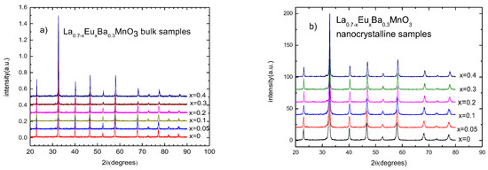
Figure 1.
X-ray diffraction patterns for (a) La0.7−xEuxMnO3 polycrystalline bulk samples and (b) La0.7−xEuxMnO3 nano-sized samples.
Rietveld refinement analysis confirms the rhombohedral structure of the parent compound for each studied sample with an R-3c space group. Figure 2 presents the values for lattice parameter (a) and cell volume (V) for all of the samples as a function of Eu content (x). As observed, with increasing substitution level, the lattice parameter becomes smaller. This is due to Eu3+ ions having a smaller ionic radius (1.206 Å) than La3+ ions (1.5 Å) [14,15]. In turn, this changes the Mn-O-Mn angle, creating distortion in the Mn-O octahedral [14].
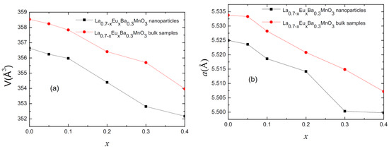
Figure 2.
(a) Plot of cell volume for polycrystalline bulk and nano-sized samples. (b) Plot of cell parameter “a” for polycrystalline bulk and nano-sized samples.
In order to understand the stability of these structures, the Goldschmidt tolerance factor was calculated using following relation [7,14]:
where RA is the radius of A cation, RB is the radius of B cation, and R0 is the radius of the anion.
It should be noted that with an increasing Eu ion content in the samples, the tolerance factor decreases slightly but remains consistent with keeping an orthorhombic/rhombohedral structure. Eu ions cause a decrease in RA and an increase in disorder [14]. In turn, this will decrease orbital overlap and the band gap. The values of the tolerance factor are within the values for an orthorhombic/rhombohedral structure [15]. The angle of Mn-O-Mn bonds increased in the parent samples for both bulk and nanocrystalline samples from 167° to 169° for x = 0.05. Furthermore, as shown in Table 1 and Table 2, the bond length of Mn-O diminishes with each additional substitution.

Table 1.
Calculated tolerance factors, Mn-O lengths, and crystallite sizes for nanocrystalline samples using the Williamson–Hall and Rietveld methods, including strain values.
Table 2.
Calculated Mn-O lengths and crystallite sizes for polycrystalline bulk samples using the Williamson–Hall and Rietveld methods, including strain values.
The Williamson–Hall (W-H) method [16] for determining crystallite sizes was used for both systems. Table 1 shows the calculation for nanocrystalline samples with an average size range of 30–55 nm for the crystallites. This agrees with the results of TEM investigation. Pictured in Figure 3, TEM shows that the average size of the particles is about 50 nm, varying between 30 nm and 70 nm. Widely used Scherrer size calculations do not take into account the strain between the grains, and thus, they tend to be lower in value. According to Williamson–Hall calculations, the size varies from 106 nm to 172 nm, while scanning electron microscopy (SEM) shows the grain size to be 3–10 μm. The same can be observed for Rietveld crystallite size results; although they are bigger than from the WH method, they are still smaller than the SEM results. This can be attributed to the fact that a single grain contains several crystallites.
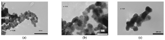
Figure 3.
Selected TEM pictures for La1−xEuxMnO3 nano-sized samples for x = 0.05 (a), x = 0.1 (b), x = 0.2 (c).
Energy dispersive X-ray spectroscopy (EDX) was also carried out for the bulk samples. As seen in Figure 4b, where a typical example is presented, the stoichiometry of heavy elements (including lanthanum, europium, barium, and manganese) is in very good agreement with the theoretical values. The distribution of the elements on the surface is considerably uniform. It is good to note here that oxygen is a much smaller atom and does not interact with X-rays nor heavier atoms [17] (pp. 279–307). For that reason, iodometry was implemented as a reliable way to calculate oxygen content.
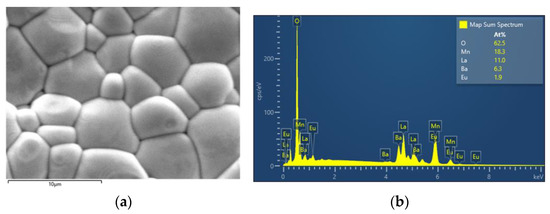
Figure 4.
(a) SEM picture of the La0.65Eu0.05Ba0.3MnO3 sample. (b) EDX for the La0.65Eu0.05Ba0.3MnO3 sample.
3.2. Oxygen Content
Iodometric titration and inductively coupled plasma atomic emission spectroscopy were used to study the oxygen content of the bulk samples.
Iodometry is a reliable and popular method of determining oxygen content in manganites [18], as it involves direct measurement of the fraction of Mn3+ vs. Mn4+ ions. In this study, all of the samples exhibited an excess of Mn3+ content. This could be attributed to the oxygen deficiency during calcination and sintering. An average of 75% Mn3+ would result in an average oxygen content of O2.97 in the range of 2.96–2.99 [19], which would affect its electrical and magnetic properties [19]. The experiment showed acceptable dispersion and error. Standard deviation is a measure of dispersion of data values, or how close they are to the “mean” value, while relative standard deviation is the percentage value of the standard deviation around the “mean”. In our study, the relative standard deviation did not exceed 2.7%, showing close proximity to the mean. Results are shown in Table 3.
Table 3.
Average oxygen content calculated using iodometry and inductively coupled plasma optical emission spectrometry (ICP-OES).
The results of iodometry were confirmed with inductively coupled plasma optical emission spectroscopy (ICP-OES) [20]. The process involves passing of the elements through a plasma of argon, which causes excitation and emission of specific wavelengths of light. The results are presented in Table 3. The average oxygen content according to ICP-OES falls well within the error limit of the iodometry results.
3.3. Electrical Measurements
An investigation of electrical resistivity at 0, 1, 2 T was carried out using the four-point probe method. The graphs are shown in Figure 5. As can be seen, the sample with x = 0.3 exhibits an expected behavior typical of a ferromagnetic manganite, with a maximum at Tp. The samples with x = 0–0.2 have similar behaviors, while the sample with x = 0.4 exhibits semi-conducting behavior. The results for Curie temperatures (TC, as obtained from magnetic measurements), Tp, the values of the resistivities in the absence of a magnetic field (ρpeak, at 0 T), and the values of magnetoresitance (MR) at Tp are presented in Table 4. Magnetoresistance was calculated using the following formula [16]:
MR% = [(ρ(H) − ρ(0))/ρ(0)] × 100,
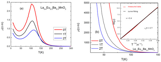
Figure 5.
Resistivity vs. temperature graphs for (a) x = 0.3 and (b) x = 0.4. The inset shows the fitting of ln(ρ) as a function of T−1/4 for μ0H = 0 T.
Table 4.
Experimental values for La0.7−xEuxBa0.3MnO3 bulk materials: electrical properties.
The first observation to be made here is that the Tp metallic–insulator transition temperature for each sample at 0 T magnetic field is lower than its TC; for example, TC (x = 0.05) = 297 K, and Tp (x = 0.05) = 256 K. This is due to the effect of grain boundaries which act as a semiconductor (or insulator) pushing the inter-grain coupling to lower temperatures [21]. When an external magnetic field is applied, the peak shifts to the right, increasing the conductive properties of the sample. This can be attributed to the lowering of spin fluctuations and to the delocalization of charge carriers caused by the applied magnetic field, which improves the double exchange interaction [22].
Each addition of a smaller-sized Eu3+ ion in place of an La3+ ion causes disorder [7]. It also changes the angle between Mn-O-Mn by “pulling” oxygen towards the A-site [23]. A decrease in the angle changes the overlap of the electron orbital, which reduces the hopping amplitude of the electrons and causes them to be more localized. This can be observed in the systematic lowering of the Tp of samples with an increasing level of substitution. For high Eu content (x = 0.4), the disorder and the reduced value of the Mn-O-Mn angle resulted in a semiconductor-like behavior of the electrical conductivity of the compound.
From the values for resistivity (ρpeak) and magnetoresistance (MRMax) in Table 4, it is eviden, that both of them tend to increase with increasing substitution level of Eu. The maximum observed resistivity for the x = 0.3 sample is 240 Ω٠cm and (MRMax) (2 T) = 63.6%, while the resistivity increases to several orders of MΩ·m for x = 0.4.
The samples with x < 0.4 have typical CMR resistivity behavior as a function of temperature and applied magnetic field, as can be seen in Figure 5, except in the low-temperature region where an upturn of resistivity occurs. The analysis of these temperature dependences is usually made both for the metallic regime before metal–insulator transition (MIT) and for the semiconducting behavior in the range of higher temperatures [24]. Within the metallic region behavior, the dominant scattering phenomena are electron-electron and electron–magnon [24] (pp. 21–32) with ρ = ρ0 + ρ2T2 + ρ4.5T4.5. At higher temperatures, after MIT, the resistivity shows semiconductor behavior and its temperature dependence can be described by using the variable range hopping (VRH) and small polaron hopping (SPH) models [25].
For the semiconducting sample, with x = 0.4 (Figure 5b), the best fit for the resistivity behavior is the expression corresponding to the VRH model for a three-dimensional system: ρ(T) = ρ0 exp (T0/T)0.25 (as shown in the inset of Figure 5b, for μ0H = 0 T), where ρ0 is the prefactor and T0 is a characteristic temperature which is related to the density of states at the Fermi level and to the localization length.
It is interesting that in spite of the semiconducting behavior, this sample shows CMR properties. This behavior suggests an electrical conduction mechanism which takes place (by tunneling) between isolated manganite grains which have negative magnetoresistance.
The behavior of resistivity at temperatures below Tp is of interest in this study. A minimum in resistivity can be observed at around 30–50 K before resistivity increases again. This behavior is exhibited by all samples except the one with the highest amount of Eu, where resistivity increases drastically below Tp. In the literature, the minimum in resistivity was partially attributed to Kondo-like effects [14]. These minima are caused by small magnetic impurities which localize electrons of opposite spin, thus increasing the scattering of conduction electrons. However, this scenario is quite different from that of polycrystalline manganites with different size grains separated by (disordered matter) grain boundaries; this rules out the hypothesis of the Kondo effect [26].
The upturn can be better explained by the combined effect of electron–electron interactions, electron–phonon scattering, and weak localization [24,27]. In addition, the disorder and strain from the grain boundaries can also act as supplementary localization factors of charge carriers. Besides these, the electrical conductivity of the grain boundaries depreciates with decreasing temperature, leading to increased resistivity. The upturn in the thermal dependence of resistivity is a consequence of both intrinsic (intragrain) effects and extrinsic grain boundary scattering/tunneling effects [28], as was also found in some other polycrystalline complex transition metal oxides. The sample with the highest Eu content exhibits a continual increase in resistivity below Tp, which can be explained by the size and quality of the grain boundaries. It is evident that grain boundaries play a dominant role in the electrical behavior of the samples.
3.4. Magnetic Properties
All of the samples exhibit ferromagnetic–paramagnetic transitions. Typical and selected magnetization vs. temperature (M(T)) plots are presented in Figure 6. Curie temperatures can be calculated from the derivative of the magnetization with respect the temperature, with the inflection point corresponding to Tc, which can be seen in Table 5, Table 6 and Table 7 [29]. With increasing Eu content x, the values of Tc gradually and systematically become lower as a result of the induced disorder. The sample with x = 0.05 has Curie temperature TC = 297 K.
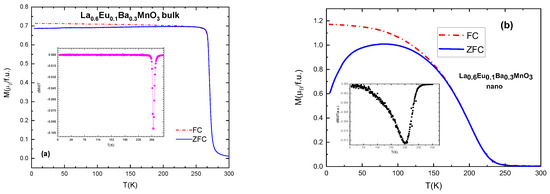
Figure 6.
(a) ZFC-FC curves and derivative of magnetization (in inset) for the bulk sample with x = 0.1; (b) ZFC-FC curves and derivative (in inset) for nanocrystalline sample with x = 0.1.
Nano-scale particles also show ferromagnetic behavior, but their TC values are lower compared to the equivalent bulk material, as shown in Figure 6. This is due to the size of particles and their ”surface effects” which occur as a result of a large surface-to-volume ratio [30], i.e., disorder effects in the surface layer of the particles which contain an increased number of broken chemical bond and other defects, resulting in spin canting and reducing the magnetic moment of the particles [31]. An average difference in TC values is 70–90 K for the samples with the same substitution level: TC (x = 0.1 bulk) = 270 K and TC (x = 0.1 nano) = 200 K. It is also interesting that the slope of the magnetization change of the M(T) curves in nanoparticles is much lower than in bulk, which can be attributed to the distribution of the particle sizes within the samples. In general, bulk material has higher values of magnetization and a narrower temperature range of the magnetic phase transition, as can be seen in Figure 6.
Arrott plots (M2 vs. H/M) allow the determination of the magnetic phase transition order [32]. According to the Banerjee criterion, positive and negative slopes of the curves correspond to second- and first-order magnetic phase transitions, respectively [28]. All of the samples exhibit positive slopes for these curves, indicating second-order magnetic phase transitions. A selected sample of Arrott plots are presented in Figure 7.
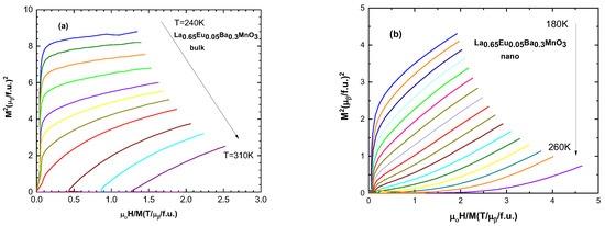
Figure 7.
Arrott plot (M2 vs. H/M) for (a) the bulk sample with x = 0.05 and for (b) the nanocrystalline sample with x = 0.05.
Arrott plots are based on Landau’s mean field theory, [33]. The Gibbs free energy around a critical point is defined as
where a and b are coefficients which depend on temperature. Minimizing the Gibbs free energy with respect to magnetization, we obtain
G (T,M) = GO + MH + aM2 + bM4 +…,
H/M = 2a + 4bM2,
According to Gibbs free energy equations, the isotherm lines must be parallel and straight, but that is not observed in Arrott plots. The problem lies in inexactness of the critical exponents [34]. β relates to spontaneous magnetization and α is related to the inverse of susceptibility χ [34,35].
These equations can be generalized as follows [34]:
where ε is the reduced temperature (T − Tc)/Tc and M0, h0/M0, and D are critical amplitudes.
MS(T) = M0 (−ε)β, T < TC,
M= D (μ0H1/δ), T = TC,
For mean field theory, we have γ = 1, β = 0.5, and δ = 3. For the 3D Heisenberg model, we have γ = 1.366, β = 0.355, and δ = 4.8. For the Ising model, we have γ = 1.24, β = 0.325, and δ = 4.82. For the tricritical mean field model, we have γ = 1, β = 0.25, and δ = 5 [24,36].
The modified Arrott plot method [35] is an iterative method. It begins with an Arrott–Noakes plot (M1/β vs. μ0H/M1/γ), which involves finding proper exponents which will make the lines parallel and straight to determine the β and γ critical exponents [10]. Spontaneous magnetization MS(T,0) is found from the intercepts of isotherms with the ordinate of the plot. The inverse of the susceptibility χ0−1(T) is taken from the intercept with the abscissa. Further fitting of these values into Equations (6)–(8) refines the values to those very close to real ones. The Widom scaling relation β + γ = β δ [10] gives the value of δ. Selected graphs for modified Arrott plots are presented in Figure 8; the data are presented in full in Table 5.
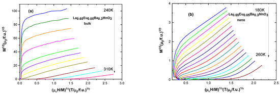
Figure 8.
Modified Arrott plots for (a) the bulk sample with x = 0.05 and for (b) the nanocrystalline sample with x = 0.05.
Table 5.
Critical exponent values for all samples.
Table 5.
Critical exponent values for all samples.
| Compound | γ | β | δ | Tc (K) | |
|---|---|---|---|---|---|
| x= 0 | bulk | 1.065 | 0.288 | 4.69 | 340 |
| x = 0.05 | bulk | 0.915 | 0.234 | 4.9 | 297 |
| x = 0.1 | bulk | 1.07 | 0.24 | 5.45 | 270 |
| x = 0.2 | bulk | 0.976 | 0.246 | 4.967 | 198 |
| x = 0.3 | bulk | 0.933 | 0.255 | 4.659 | 142 |
| x= 0.4 | bulk | 1.022 | 0.249 | 5.104 | 99 |
| x = 0 | nano | 1.823 | 0.493 | 4.698 | 263 |
| x= 0.05 | nano | 1.968 | 0.548 | 4.589 | 220 |
| x = 0.1 | nano | 1.867 | 0.521 | 4.584 | 200 |
| x = 0.2 | nano | 1.755 | 0.477 | 4.679 | 136 |
| x= 0.3 | nano | 1.931 | 0.537 | 4.596 | 90 |
| x = 0.4 | nano | 1.789 | 0.512 | 4.49 | 64 |
| Mean field model | 1 | 0.5 | 3 | ||
| 3D Heisenberg model | 1.366 | 0.355 | 4.8 | ||
| Ising model | 1.24 | 0.325 | 4.82 | ||
| Tricritical mean field model | 1 | 0.25 | 5 | ||
Figure 9 shows the values for critical exponents for two of the samples: one of bulk and one of nano-scale. It is evident that the bulk samples are more closely governed by the tricritical mean field model (β = 0.234, γ = 0.915, δ = 4.9) for ferromagnets and the nanoparticle samples are governed by the 3D Heisenberg model (β = 0.548, γ = 1.968, δ = 4.589), rather than mean field theory model.
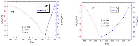
Figure 9.
Calculated values for critical exponents for (a) the bulk sample with x = 0.05 (b) for the nanocrystalline sample with x = 0.05.
Usually, the 3D Heisenberg model can describe the critical properties of the short-range interactions in doped manganites, together with other theoretical models, such as the mean field and tricritical mean field models. The critical exponent values are related to the range of exchange interaction J(r), spin, and system dimensionality. Within renormalization group theory [37], J(r) = 1/rd+σ (d—dimensionality of the system; σ—range of interaction). For σ greater than 2, the 3D Heisenberg model is valid. For σ < 3/2, the mean field theory of long-range interaction is valid. For an intermediate range, a different universality class occurs. For the tricritical point, the critical exponents are universal: β = 0.25, γ = 1, and δ = 5. The tricritical point sets a boundary between two different ranges of order phase transitions. In this study, we focused on the general different magnetic properties of nano- and bulk polycrystalline manganites, not on their high-detail magnetic critical behavior. The modified Arrott plot (MAP) method is very accurate, and its agreement with the Kouvel–Fisher (KF) method and critical isotherm (CI) plots is usually quite remarkable [24,38]; indeed, some authors only analyze these data [39]. This is why we report here the results obtained by using MAP analysis.
All of the samples exhibit a very small coercive field as evident from hysteresis curves, with the largest values of 170 Oe for x = 0.05 bulk and 960 Oe for x = 0.4 nano-sample. This can be largely attributed to low anisotropy and lack of pinning sites [40]. Nanoparticles show greater coercivity than their bulk counterparts, as shown in Table 6 and Table 7. It has been found, in previous works, that nanoparticle coercivity tends to increase with a decreasing size in the multi-domain range, and then it decreases in the single-domain range until it reaches a superparamagnetic state, when it becomes zero [41]. Low coercivity is of utmost importance for the magnetocaloric effect.
Suitability for cooling via the magnetocaloric effect is determined by the value of magnetic entropy change in the material [40]. An appropriate ratio between Mn3+ and Mn4+ is needed for optimal ferromagnetic behavior. About 30% Mn4+ gives the best results [8]. When the number of charge carries increases, the risk of entering a charge ordered state occurs, where electron hopping is prohibited by rigid atomic distribution [8]. For second-order phase transitions (which were established via Arrott plots earlier), magnetic entropy change (ΔSM) can be calculated from magnetization M (μ0H) isotherm data and is approximated by the following equation [42]:
To estimate the magnetocaloric effect, we plot −ΔSM vs. T (temperature) for values of external magnetic field (μ0H) of 1, 2, 3, 4 T in Figure 10. Furthermore, relative cooling power (RCP) is calculated as the product of entropy change (ΔSM) and temperature change at half maximum (δTFWHM)
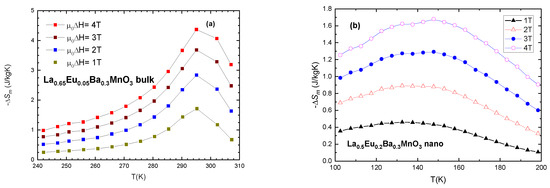
Figure 10.
Magnetic entropy change vs. temperature for selected samples: (a) x = 0.05 bulk and (b) x = 0.2 nanocrystalline sample.
Table 6 shows the progression of magnetic entropy change in bulk samples and Table 7 shows the same for nano-sized samples. It is evident that maximum magnetic entropy change occurs at temperatures very close to Tc. Of interest in both systems is the fact that both bulk and nanocrystalline samples with x ≤ 0.3 exhibit RCP values which are in the range of the values recommended for magnetocaloric materials [43]. An interesting note to be made is that the values of Relative Cooling Power (RCP) for similar samples are comparable to each other. RCP (x = 0.2) bulk = 212.4 9 (J/kg) and RCP (x = 0.2) nano = 218.6 (J/kg) (Table 6 and Table 7) for μ0ΔH = 4 T. The values for the maximum magnetic entropy change are very good in comparison with similar compounds presented in the literature as potential magnetocaloric materials [10,44]. Another interesting and useful note is the shape of the curves of magnetic entropy change for bulk and nanocrystalline samples. The bulk material exhibits a sharp curve, while nanoparticles have lower but wider curves. This is due to the size distribution of the nanoparticles and their separation. While the peak entropy change |ΔSM| for bulk material is higher (4.2 J/KgK) than for nano-material (1.63 J/kgK), the width of the temperature change (δTFWHM) is reversed, with 37 K for bulk and 95 K for equivalent samples (x = 0.05) when μ0ΔH = 4 T. This fact can be useful for the cooling industry, where a wider range of applications is preferable.
Table 6.
Experimental values for La0.7−xEuxBa0.3MnO3 bulk materials: magnetic measurements.
Table 6.
Experimental values for La0.7−xEuxBa0.3MnO3 bulk materials: magnetic measurements.
| Compound (Bulk) | TC (K) | Ms (μB/f.u.) | Hci (Oe) | |ΔSM| (J/kgK) μ0ΔH = 1 T | |ΔSM| (J/kgK) μ0ΔH = 4 T | RCP (S) (J/kgK) μ0ΔH = 1 T | RCP (S) (J/kgK) μ0ΔH = 4 T | Refs |
|---|---|---|---|---|---|---|---|---|
| La0.7Ba0.3MnO3 | 340 | 4.04 | 200 | 1.33 | 3.5 | 53.7 | 158.4 | This work |
| La0.65Eu0.05Ba0.3MnO3 | 297 | 3.87 | 172 | 1.71 | 4.2 | 42.7 | 155.4 | This work |
| La0.6Eu0.1Ba0.3MnO3 | 270 | 3.84 | 63 | 1.6 | 4.1 | 40 | 187.7 | This work |
| La0.5Eu0.2Ba0.3MnO3 | 198 | 3.7 | 67 | 1.41 | 3.7 | 38.1 | 212.6 | This work |
| La0.4Eu0.3Ba0.3MnO3 | 142 | 3.78 | 66 | 1.7 | 3.5 | 42.6 | 176.4 | This work |
| La0.3Eu0.4Ba0.3MnO3 | 99 | 3.46 | 120 | 1.02 | 2.83 | 25.7 | 133.3 | This work |
| La0.7Ca0.3MnO3 | 256 | 1.38 | 41 | [10] | ||||
| La0.7Sr0.3MnO3 | 365 | - | 4.44 (5 T) | 128 (5 T) | [10] | |||
| La0.6Nd0.1Ca0.3MnO3 | 233 | 1.95 | 37 | [10] | ||||
| Gd5Si2Ge2 | 276 | - | 18 (5 T) | - | 535 (5 T) | [10] | ||
| Gd | 293 | 2.8 | 35 | [10] |
Table 7.
Experimental values for La0.7−xEuxBa0.3MnO3 nano materials.
Table 7.
Experimental values for La0.7−xEuxBa0.3MnO3 nano materials.
| Compound (Nano) | Tc (K) | Ms (μB/f.u.) | Hci (Oe) | |ΔSM| (J/kgK) μ0ΔH = 1 T | |ΔSM| (J/kgK) μ0ΔH = 4 T | RCP(S) (J/kgK) μ0ΔH = 1 T | RCP(S) (J/kgK) μ0ΔH = 1 T | Refs |
|---|---|---|---|---|---|---|---|---|
| La0.7Ba0.3MnO3 | 263 | 2.79 | 4800 | 1.04 | 1.37 | 105.4 | 130.1 | This work |
| La0.65Eu0.05Ba0.3MnO3 | 220 | 2.95 | 410 | 0.43 | 1.63 | 43.3 | 155.6 | This work |
| La0.6Eu0.1Ba0.3MnO3 | 200 | 2.6 | 390 | 0.93 | 1.23 | 93.5 | 135.3 | This work |
| La0.5Eu0.2Ba0.3MnO3 | 136 | 2.96 | 280 | 0.46 | 1.68 | 47.8 | 218.4 | This work |
| La0.4Eu0.3Ba0.3MnO3 | 90 | 2.3 | 590 | 0.39 | 1.99 | 38.3 | 187.7 | This work |
| La0.3Eu0.4Ba0.3MnO3 | 64 | 2.09 | 960 | 0.25 | 1.09 | 23.3 | 119.9 | This work |
| La0.67Ca0.33MnO3 | 260 | 0.97 (5 T) | 27 (5 T) | [45] | ||||
| Pr0.65(Ca0.6Sr0.4)0.35MnO3 | 220 | 0.75 | 21.8 | [46] | ||||
| La0.6Sr0.4MnO3 | 365 | 1.5 | 66 | [47] |
4. Conclusions
The compounds La0.7−xEuxBa0.3MnO3 (x = 0, 0.05, 0.1, 0.2, 0.3, 0.4) were synthetized by solid-state reaction to produce a bulk material whose crystalline structure and morphology were investigated by XRD and SEM. The sol-gel method was used to produce nano-scale particles, which were analyzed by XRD and TEM, showing an average size of 30–70 nm. Both systems are single phase, with rhombohedral (R-3c) lattice symmetry. Cell parameters diminish with addition of Eu in the lattice structure. Mn-O bond length tends to shorten with an increasing level of Eu, and the addition of Eu increases the angle Mn-O-Mn. ZFC-FC plots suggest single magnetic phase and low magnetic anisotropy. The sample with x = 0.05 shows a magnetic phase transition at 297 K for bulk compound, while the La0.7Ba0.3MnO3 nanoparticle sample has TC = 263 K. Both systems show very small coercivity, with nano-sized samples being slightly larger: 63 Oe for the bulk sample with x = 0.1 and 390 Oe for the corresponding nanocrystalline sample. Iodometry was used in order to estimate oxygen content in samples, showing a lower concentration of Mn4+ ions, leading to the lowest value of oxygen content to be O2.97±0.02 for the x = 0.4 sample. General oxygen deficiency was confirmed by inductively coupled plasma optical emission spectrometry (ICP-OES). The samples with x < 0.4 show metallic–insulator transition at a temperature Tp lower than magnetic transition temperatures Tc. The sample with x = 0.4 exhibits increasing resistivity with decreasing temperature below 160 K, suggesting either the ferromagnetic clusters are non-metallic or they are too small to compensate the increase of resistivity induced by disorder. All samples show negative magnetoresistance. The sample with x = 0.3 exhibits magnetoresistance MR (2 T) = 63.6%. Arrott plots confirm second-order magnetic phase transition for all of the samples. Modified Arrott plot analysis revealed the critical exponents for bulk samples to be in the tricritical mean field model range and in the 3D Heisenberg model range for nanocrystalline samples. The maximum magnetic entropy change of 4.2 J/kgK was observed for the x = 0.05 bulk sample for µ0ΔH = 4 T. Nanocrystalline samples exhibit lower peak magnetic entropy change (1.63 J/kgK for x = 0.05), but Tfwhm exceeds 100 K (130K for x = 0.2). Relative cooling power RCP is comparable between equivalent samples for both systems: 212.4 J/kg for x = 0.3 in nanocrystalline samples and 212.6 J/kg for bulk. The value of RCP close to room temperature phase transition TC = 297 K for the bulk sample La0.65Eu0.05Ba0.3MnO3 is 155.4 J/Kg, possessing the required parameters of a magnetocaloric material. Since the temperature range (δTFWHM) for nano-sized samples La0.7Ba0.3MnO3 and La0.65Eu0.05Ba0.3MnO3 covers a wide range (95 K) including room temperature, they may be used in multistep refrigeration processes. However, we should be cautious in taking high RCP values for nano-materials at face value [48]; potentially, fewer compounds would be necessary for use in stacks of refrigeration systems. This wide range of effective cooling in nanoparticles together with high entropy change in bulk material can be combined for suitable commercial cooling.
Author Contributions
R.A., conceptualization, investigation, methodology, writing—original draft, writing—review and editing, visualization, supervision; R.H., R.B., E.C., F.P. and T.F., methodology, investigation, writing—review and editing; I.G.D., conceptualization, investigation, methodology, visualization, supervision, writing—review and editing. All authors have read and agreed to the published version of the manuscript.
Funding
This research received no external funding.
Institutional Review Board Statement
Not applicable.
Informed Consent Statement
Not applicable.
Data Availability Statement
Data presented in this study are available in this article.
Acknowledgments
The authors acknowledge Ioan Ursu from the Faculty of Physics, Babes Bolyai University, for assistance.
Conflicts of Interest
The authors declare no conflict of interest.
References
- Fidler, J.C. A History of Refrigeration throughout the World. Int. J. Refrig. 1979, 2, 249–250. [Google Scholar] [CrossRef]
- Briley, G.C. A History of Refrigeration. ASHRAE J. 2004, 46, S31–S34. [Google Scholar]
- Gschneidner, K.A.; Pecharsky, V.K. Thirty Years of near Room Temperature Magnetic Cooling: Where We Are Today and Future Prospects. Int. J. Refrig. 2008, 31, 945–961. [Google Scholar] [CrossRef]
- Dorin, B.R.; Avsec, J.; Plesca, A. The Efficiency of Magnetic Refrigeration and a Comparison with Compresor Refrigeration Systems. J. Energy Tecnol. 2018, 11, 59–69. [Google Scholar]
- Moya, X.; Kar-Narayan, S.; Mathur, N.D. Caloric Materials near Ferroic Phase Transitions. Nat. Mater. 2014, 13, 439–450. [Google Scholar] [CrossRef]
- Dagotto, E.; Hotta, T.; Moreo, A. Colossal Magnetoresistant Materials: The Key Role of Phase Separation. Phys. Rep. 2001, 344, 1–153. [Google Scholar] [CrossRef]
- Dagotto, E. Nanoscale Phase Separation and Colossal Magnetoresistance, 1st ed.; Springer Science & Business Media: New York, NY, USA, 2002; pp. 271–284. [Google Scholar]
- Coey, J.M.D.; Viret, M.; Von Molnár, S. Mixed-Valence Manganites. Adv. Phys. 1999, 48, 167–293. [Google Scholar] [CrossRef]
- Rostamnejadi, A.; Venkatesan, M.; Alaria, J.; Boese, M.; Kameli, P.; Salamati, H.; Coey, J.M.D. Conventional and Inverse Magnetocaloric Effects in La0.45Sr 0.55MnO3 Nanoparticles. J. Appl. Phys. 2011, 110, 043905. [Google Scholar] [CrossRef]
- Varvescu, A.; Deac, I.G. Critical Magnetic Behavior and Large Magnetocaloric Effect in Pr0.67Ba0.33MnO3 Perovskite Manganite. Phys. B Condens. Matter 2015, 470–471, 96–101. [Google Scholar] [CrossRef]
- Weng, S.; Zhang, C.; Han, H. 3D-Heisenberg Ferromagnetic Characteristics in a La0.67 Ba0.33 MnO3 Film on SrTiO3. Eur. Phys. J. B 2021, 94, 91. [Google Scholar] [CrossRef]
- Liedienov, N.A.; Pashchenko, A.V.; Pashchenko, V.P.; Prokopenko, V.K.; Revenko, Y.F. Structure defects, phase transitions, magnetic resonance and magneto-transport properties of La0.6–xEuxSr0.3Mn1.1O3–δ ceramics. Low Temp. Phys. 2016, 42, 1102–1111. [Google Scholar] [CrossRef]
- Amaral, J.S.; Reis, M.S.; Amaral, V.S.; Mendonca, T.M.; Araujo, J.P.; Sa, M.A.; Tavares, P.B.; Vieira, J.M. Magnetocaloric effect in Er- and Eu-substituted ferromagneticLa-Sr manganites. J Magn. Magn. Mat. 2009, 290, 686–689. [Google Scholar]
- Raju, K.; Manjunathrao, S.; Venugopal Reddy, P. Correlation between Charge, Spin and Lattice in La-Eu-Sr Manganites. J. Low Temp. Phys. 2012, 168, 334–349. [Google Scholar] [CrossRef]
- Rao, C.N.R. Perovskites. In Encyclopedia of Physical Science and Technology; Elsevier: Amsterdam, The Netherlands, 2003; pp. 707–714. [Google Scholar]
- Nath, D.; Singh, F.; Das, R. X-Ray Diffraction Analysis by Williamson-Hall, Halder-Wagner and Size-Strain Plot Methods of CdSe Nanoparticles—A Comparative Study. Mater. Chem. Phys. 2020, 239, 2764–2772. [Google Scholar] [CrossRef]
- Wolfgong, W.J. Chemical Analysis Techniques for Failure Analysis. In Handbook of Materials Failure Analysis with Case Studies from the Aerospace and Automotive Industries; Butterworth-Heinemann: Oxford, UK, 2016; pp. 279–307. [Google Scholar]
- Licci, F.; Turilli, G.; Ferro, P. Determination of Manganese Valence in Complex La-Mn Perovskites. J. Magn. Magn. Mater. 1996, 164, L268–L272. [Google Scholar] [CrossRef]
- Tali, R. Determination of Average Oxidation State of Mn in ScMnO3 and CaMnO3 by Using Iodometric Titration. Damascus Univ. J. Basic Sci. 2007, 23, 9–19. [Google Scholar]
- Covaci, E.; Senila, M.; Ponta, M.; Frentiu, T. Analitical performance and validation of optical emission and atomic absorption spectrometry methods for multielemental determination in vegetables and fruits. Rev. Roum. Chim. 2020, 65, 735–745. [Google Scholar] [CrossRef]
- Deac, I.G.; Tetean, R.; Burzo, E. Phase Separation, Transport and Magnetic Properties of La2/3A1/3Mn1−XCoxO3, A = Ca, Sr (0.5 ≤ x ≤ 1). Phys. B Condens. Matter 2008, 403, 1622–1624. [Google Scholar] [CrossRef]
- Gross, R.; Alff, L.; Büchner, B.; Freitag, B.H.; Höfener, C.; Klein, J.; Lu, Y.; Mader, W.; Philipp, J.B.; Rao, M.S.R.; et al. Physics of Grain Boundaries in the Colossal Magnetoresistance Manganites. J. Magn. Magn. Mater. 2000, 211, 150–159. [Google Scholar] [CrossRef]
- Raju, K.; Pavan Kumar, N.; Venugopal Reddy, P.; Yoon, D.H. Influence of Eu Doping on Magnetocaloric Behavior of La0.67Sr0.33MnO3. Phys. Lett. Sect. A Gen. At. Solid State Phys. 2015, 379, 1178–1182. [Google Scholar] [CrossRef]
- Kubo, K.; Ohata, N. A Quantum Theory of Double Exchange. J. Phys. Soc. Jpn. 1972, 33, 21–32. [Google Scholar] [CrossRef]
- Liedienov, N.A.; Wei, Z.; Kalita, V.M.; Pashchenko, A.V.; Li, Q.; Fesych, I.V.; Turchenko, V.A.; Hou, C.; Wei, X.; Liu, B.; et al. Spin-dependent magnetism and superparamagnetic contribution to the magnetocaloric effect of non-stoichiometric manganite nanoparticles. Appl. Mater. Today 2022, 26, 101340. [Google Scholar] [CrossRef]
- Panwar, N.; Pandya, D.K.; Agarwal, S.K. Magneto-Transport and Magnetization Studies of Pr2/3Ba 1/3MnO3:Ag2O Composite Manganites. J. Phys. Condens. Matter 2007, 19, 456224. [Google Scholar] [CrossRef]
- Panwar, N.; Pandya, D.K.; Rao, A.; Wu, K.K.; Kaurav, N.; Kuo, Y.K.; Agarwal, S.K. Electrical and Thermal Properties of Pr 2/3(Ba1-XCsx)1/3MnO 3 Manganites. Eur. Phys. J. B 2008, 65, 179–186. [Google Scholar] [CrossRef]
- Banerjee, B.K. On a Generalised Approach to First and Second Order Magnetic Transitions. Phys. Lett. 1964, 12, 16–17. [Google Scholar] [CrossRef]
- Joy, P.A.; Anil Kumar, P.S.; Date, S.K. The Relationship between Field-Cooled and Zero-Field-Cooled Susceptibilities of Some Ordered Magnetic Systems. J. Phys. Condens. Matter 1998, 10, 11049–11054. [Google Scholar] [CrossRef]
- Arun, B.; Suneesh, M.V.; Vasundhara, M. Comparative Study of Magnetic Ordering and Electrical Transport in Bulk and Nano-Grained Nd0.67Sr0.33MnO3 Manganites. J. Magn. Magn. Mater. 2016, 418, 265–272. [Google Scholar] [CrossRef]
- Peters, J.A. Relaxivity of Manganese Ferrite Nanoparticles. Prog. Nucl. Magn. Reson. Spectrosc. 2020, 120, 72–94. [Google Scholar] [CrossRef]
- Arrott, A. Criterion for Ferromagnetism from Observations of Magnetic Isotherms. Phys.Rev. 1957, 108, 1394–1396. [Google Scholar] [CrossRef]
- Jeddi, M.; Gharsallah, H.; Bejar, M.; Bekri, M.; Dhahri, E.; Hlil, E.K. Magnetocaloric Study, Critical Behavior and Spontaneous Magnetization Estimation in La0.6Ca0.3Sr0.1MnO3 Perovskite. RSC Adv. 2018, 8, 9430–9439. [Google Scholar] [CrossRef]
- Stanley, H.E. Introduction to Phase Transitions and Critical Phenomena; Oxford University Press: Oxford, UK, 1987; pp. 7–10. [Google Scholar]
- Arrott, A.; Noakes, J.E. Approximate Equation of State for Nickel Near Its Critical Temperature. Phys. Rev. Lett. 1967, 19, 786–789. [Google Scholar] [CrossRef]
- Pathria, R.K.; Beale, P.D. Phase Transitions: Criticality, Universality, and Scaling. In Statistical Mechanics; Elsevier: Amsterdam, The Netherlands, 2022; pp. 417–486. [Google Scholar]
- Fisher, M.E.; Ma, S.K.; Nickel, B.G. Critical Exponents for Long-Range Interactions. Phys. Rev. Lett. 1972, 29, 917. [Google Scholar] [CrossRef]
- Smari, M.; Walha, I.; Omri, A.; Rousseau, J.J.; Dhari, E.; Hlil, E.K. Critical parameters near the ferromagnetic–paramagnetic phase transition in La0.5Ca0.5−xAgxMnO3 compounds (0.1 ≤ x ≤ 0.2). Ceram. Int. 2014, 40, 8945–8951. [Google Scholar] [CrossRef]
- Kim, D.; Revaz, B.; Zink, B.L.; Hellman, F.; Rhyne, J.J.; Mitchell, J.F. Tri-critical Point and the Doping Dependence of the Order of the Ferromagnetic Phase Transition of La1−xCaxMnO3. Phys. Rev. Lett. 2002, 89, 227202. [Google Scholar] [CrossRef] [PubMed]
- Zverev, V.; Tishin, A.M. Magnetocaloric Effect: From Theory to Practice. In Reference Module in Materials Science and Materials Engineering; Elsevier: Amsterdam, The Nederlands, 2016; pp. 5035–5041. [Google Scholar] [CrossRef]
- Majumder, D.D.; Majumder, D.D.; Karan, S. Magnetic Properties of Ceramic Nanocomposites. In Ceramic Nanocomposites; Woodhead Publishing Series in Composites Science and Engineering; Banerjee, R., Manna, I., Eds.; Elsevier B.V.: Amsterdam, The Netherlands, 2013; pp. 51–91. [Google Scholar] [CrossRef]
- Souca, G.; Iamandi, S.; Mazilu, C.; Dudric, R.; Tetean, R. Magnetocaloric Effect and Magnetic Properties of Pr1-XCexCo3 Compounds. Stud. Univ. Babeș-Bolyai Phys. 2018, 63, 9–18. [Google Scholar] [CrossRef]
- Naik, V.B.; Barik, S.K.; Mahendiran, R.; Raveau, B. Magnetic and Calorimetric Investigations of Inverse Magnetocaloric Effect in Pr0.46 Sr0.54 MnO3. Appl. Phys. Lett. 2011, 98, 112506. [Google Scholar] [CrossRef]
- Gong, Z.; Xu, W.; Liedienov, N.A.; Butenko, D.S.; Zatovsky, I.V.; Gural’skiy, I.A.; Wei, Z.; Li, Q.; Liu, B.; Batman, Y.A.; et al. Expansion of the multifunctionality in off-stoichiometric manganites using post-annealing and high pressure: Physical and electrochemical studies. Phys Chem. Chem. Phys. 2002, 24, 21872–21885. [Google Scholar] [CrossRef]
- Hueso, L.E.; Sande, P.; Miguéns, D.R.; Rivas, J.; Rivadulla, F.; López-Quintela, M.A. Tuning of the magnetocaloric effect in nanoparticles synthesized by sol–gel techniques. J. Appl. Phys. 2002, 91, 9943–9947. [Google Scholar] [CrossRef]
- Anis, B.; Tapas, S.; Banerjee, S.; Das, I. Magnetocaloric properties of nanocrystalline Pr0.65(Ca0.6Sr0.4)0.35MnO3. J. Appl. Phys. 2008, 103, 013912. [Google Scholar] [CrossRef]
- Ehsani, M.H.; Kameli, P.; Ghazi, M.E.; Razavi, F.S.; Taheri, M. Tunable magnetic and magnetocaloric properties of La0.6Sr0.4MnO3 nanoparticles. J. Appl. Phys. 2013, 114, 223907. [Google Scholar] [CrossRef]
- Griffith, L.D.; Mudryk, Y.; Slaughter, J.; Pecharsky, V.K. Material-based figure of merit for caloric materials. J. Appl. Phys. 2018, 123, 034902. [Google Scholar] [CrossRef]


Publisher’s Note: MDPI stays neutral with regard to jurisdictional claims in published maps and institutional affiliations. |
© 2022 by the authors. Licensee MDPI, Basel, Switzerland. This article is an open access article distributed under the terms and conditions of the Creative Commons Attribution (CC BY) license (https://creativecommons.org/licenses/by/4.0/).