2.2. Rolling Process
Rolling was carried out in Liuzhou Iron and Steel Co., Guangxi Province. The diameter of the composite billet was 159 mm, the thickness of the stainless steel pipe was 6 mm, and the diameter of the finished bar was 28 mm. The complete rolling line included 14 rolling mills and 2 flying shears. The rolling steps of the clad rebar are shown below. First, the composite billet was placed in a walking beam furnace for heating at 1250 °C for 3 h. After heating, the clad rebar was rolled using a rolling mill and air-cooled to room temperature. It is worth noting that the cooling water was closed during the whole rolling process for safeguarding the full recrystallization of clad rebar.
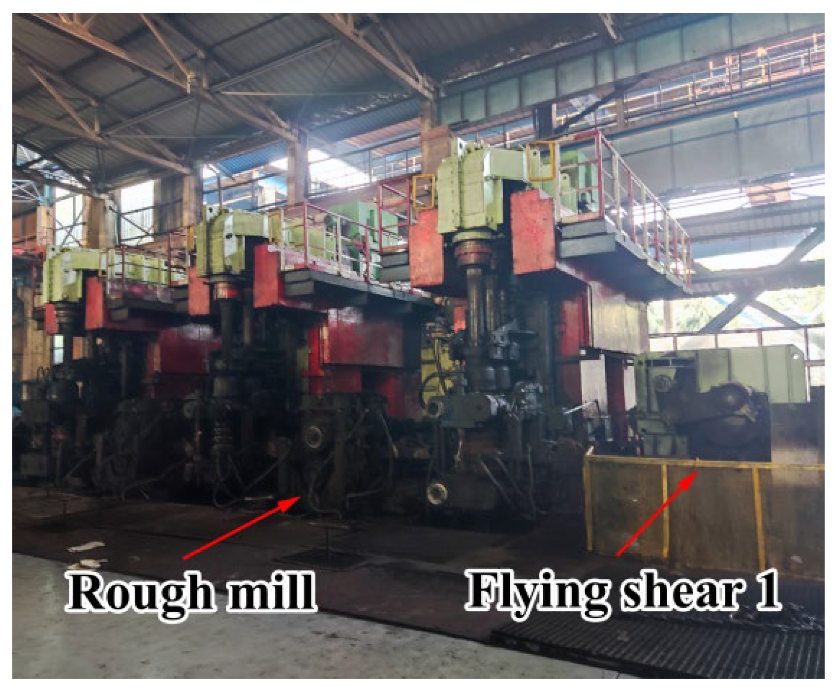
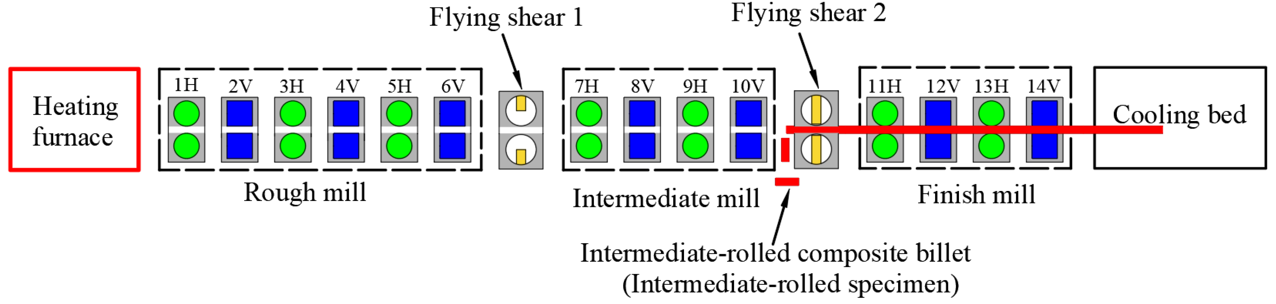
Figure 1 shows a schematic of the rough-rolling unit and the first flying shear arrangement, while
Figure 2 shows a schematic of the intermediate-rolling unit and the second flying shear arrangement.
Table 2 shows the rolling parameters of the clad rebar.
The rough-rolled composite billets were prepared as follows. When the composite billet “head” reached the first flying shear position, a command was issued through the central control console and the flying shear quickly cut the billet “head”. A total of two specimens, each approximately 1 m long, were cut.
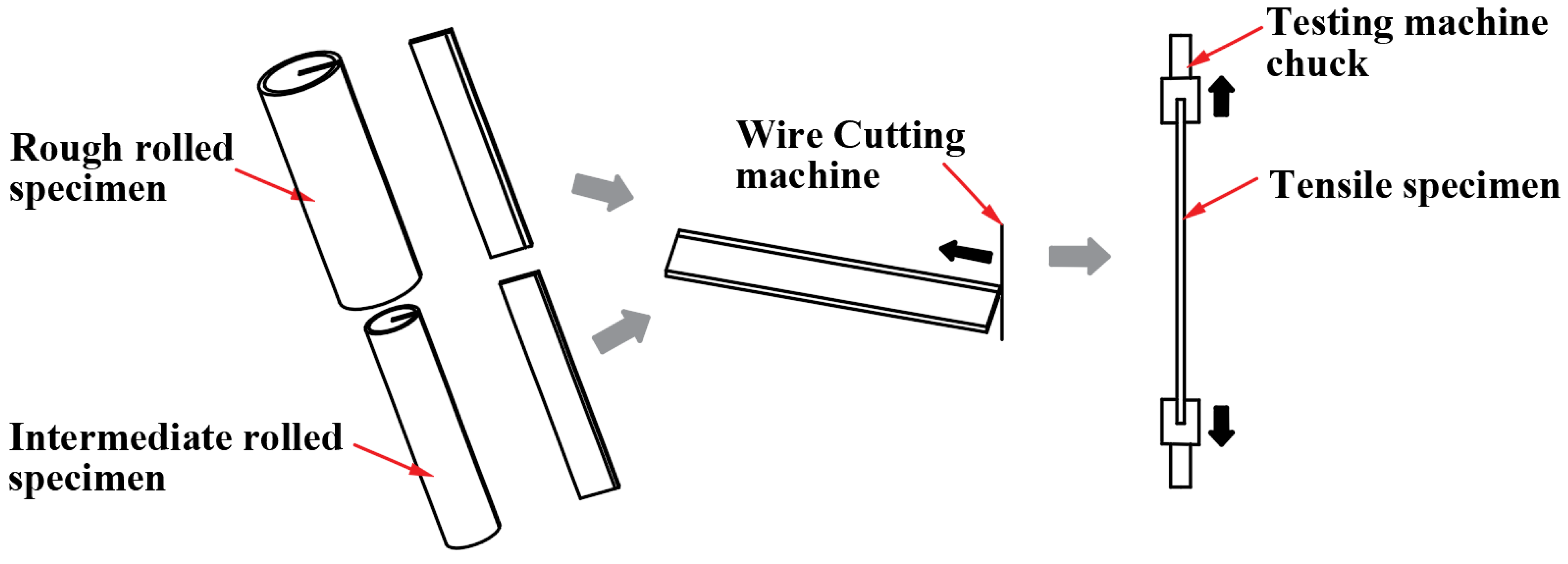
Figure 3 shows a schematic of the rough-rolling and specimen-cutting process.
Figure 4 shows a schematic of the intermediate-rolling and specimen-cutting process. The intermediate-rolled composite billets were prepared as follows. When the composite billet “tail” reached the position of the second flying shear, a command was issued through the central console and the flying shear quickly cut the billet “tail”. A total of two specimens, each approximately 1.5 m long, were cut.
The rough- and intermediate-rolled specimens were air-cooled to room temperature, numbered, and packed.
Figure 5 shows the surface morphology of the rough- and intermediate-rolled specimens and clad rebar. According to the hole pattern provided by Liuzhou Iron and Steel Co., the cumulative reduction rates corresponding to the rough- and intermediate-rolled specimens were 47.5% and 73.3%, respectively; moreover, the cumulative reduction rate corresponding to the finished clad rebar was 82.3%.
2.3. Detection Methods
The machine vision method was employed to determine the stainless steel percentage of each specimen (i.e., rough- and intermediate-rolled specimens and clad rebar) as follows. First, a 33UX287 industrial camera (The Imaging Source, New Taipei City, Taiwan, China) was used to image the end-face of the specimens. The images obtained were then subjected to grayscale processing, noise reduction, adaptive thresholding, canny edge detection, and cladding area calculation. Finally, the stainless steel occupancy ratio was obtained.
The method proposed in reference [
22] was used to calculate the average cladding thickness. First, the end-face profiles of the specimens were divided into 20 equal parts along the circumference. The cladding thickness corresponding to each part was obtained using a CAD (Autodesk company, San Rafael, CA, USA) measurement tool, and the average of these measurements was calculated.
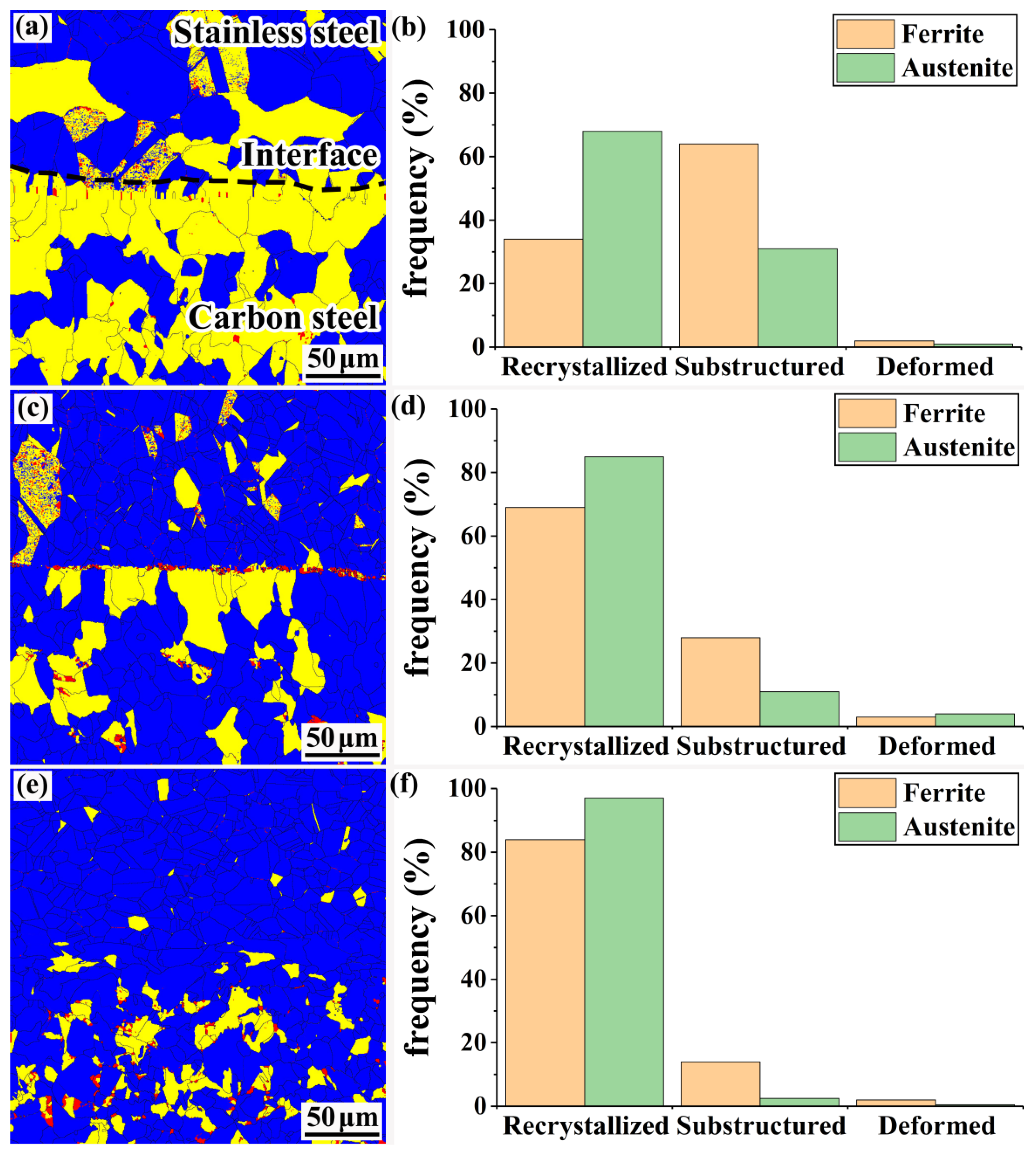
Electron backscatter diffraction (Carl Zeiss AG, Oberkochen, Germany) was used to observe and count the composite interface grain size, dislocation density, and percentage of recrystallized grains. Here, the scan step was 200 μm. The specific steps are as follows: the composite interface image was first obtained with the help of the electron backscatter diffraction and then imported into Channel5 software for calculating the grain sizes of ferrite and austenite with the grain size statistical function of the software.
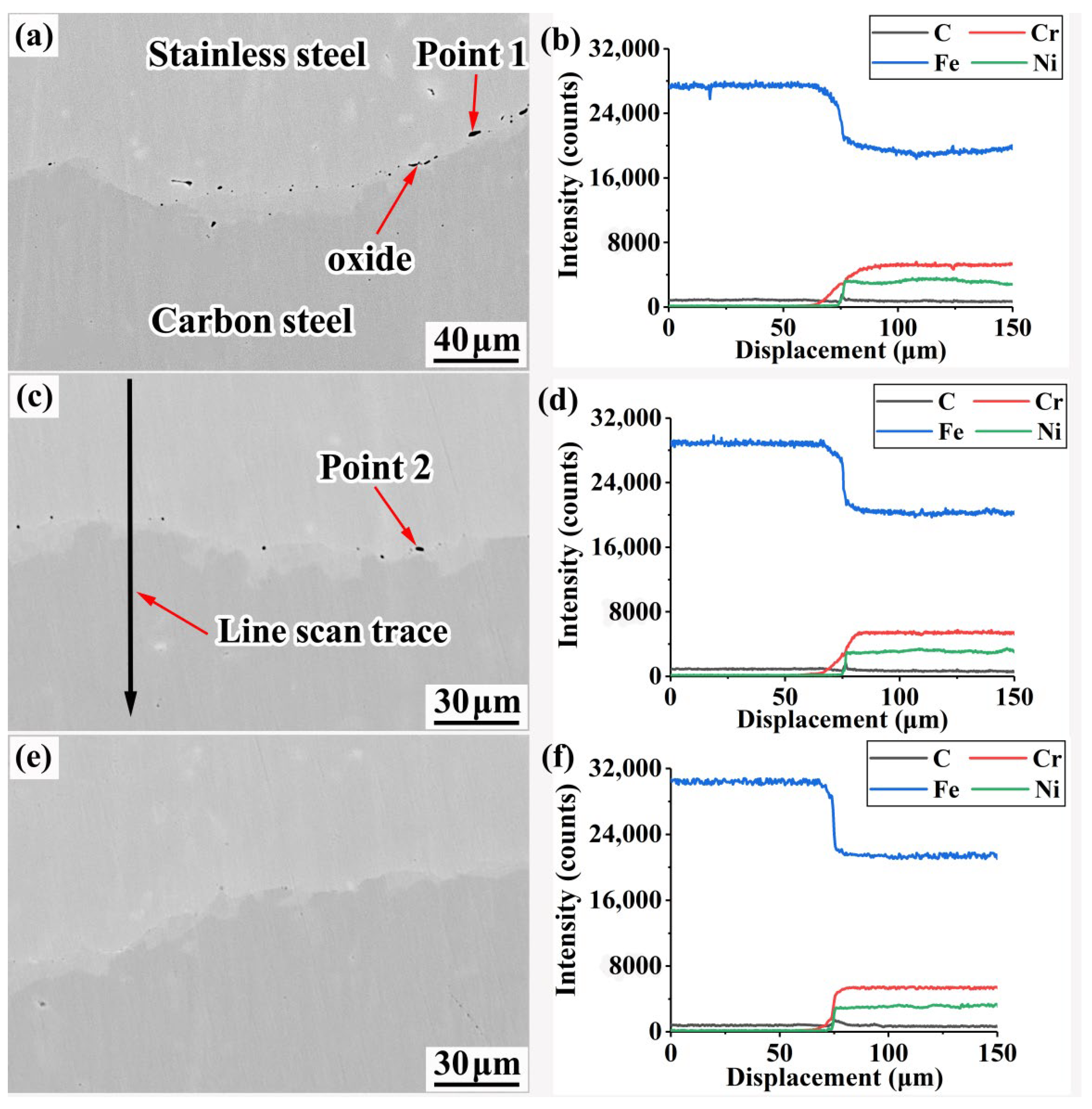
A SOPTOP optical microscope and JXA-8230 electron probe (Japan Electronics Co., Akishima-shi, Japan) were used to observe the metallographic organization and distribution of each alloying element in the composite interface, respectively.
A high-temperature Vickers hardness test system (Fuzhen Technology (Beijing) Co., Beijing, China) was used to assess the microhardness of the composite interface; here, the test load was 50 g.
The bond strength of the composite interface was tested using the method proposed in reference [
23].
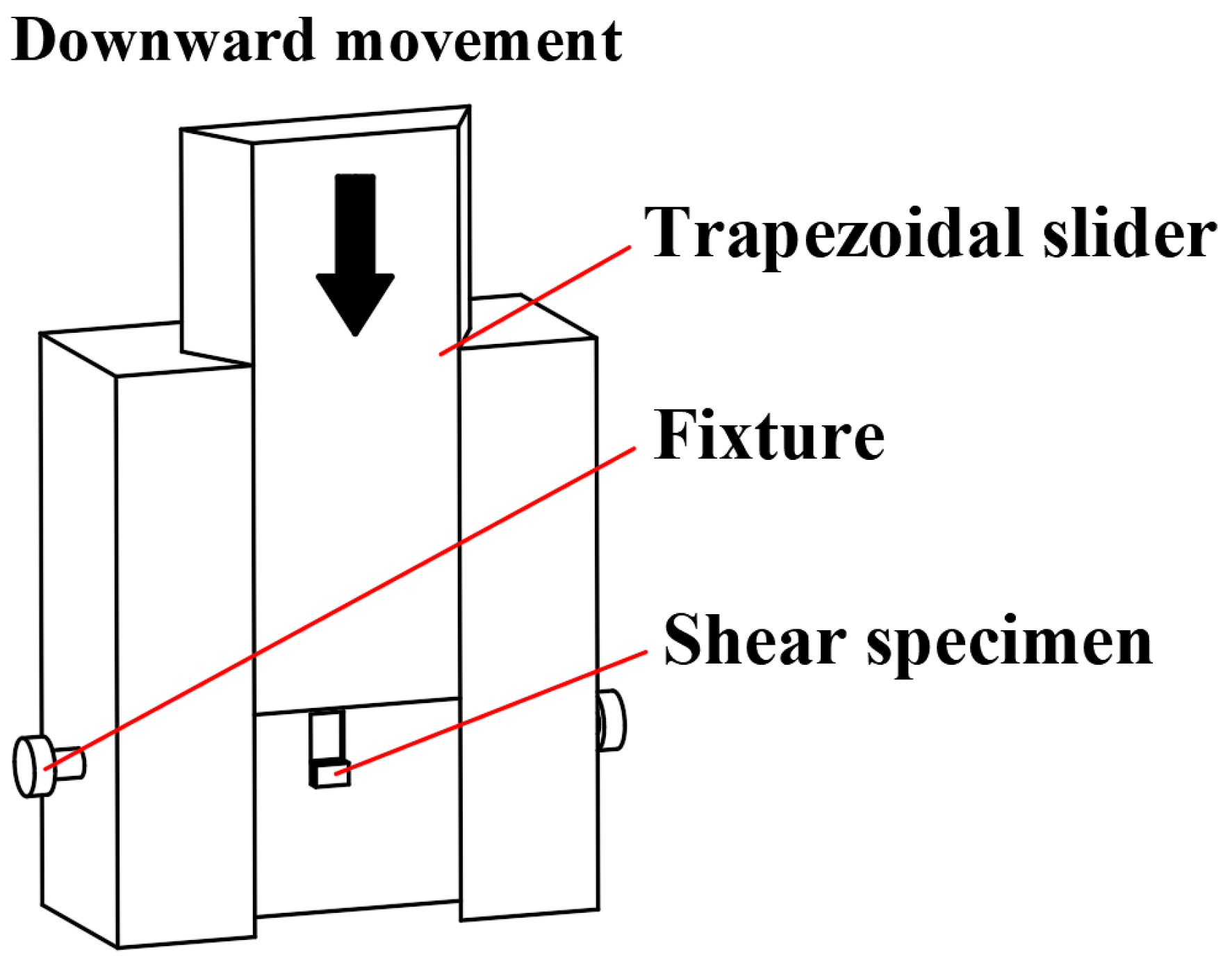
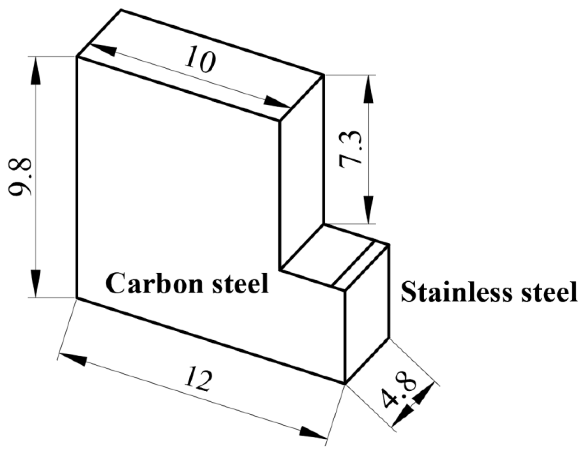
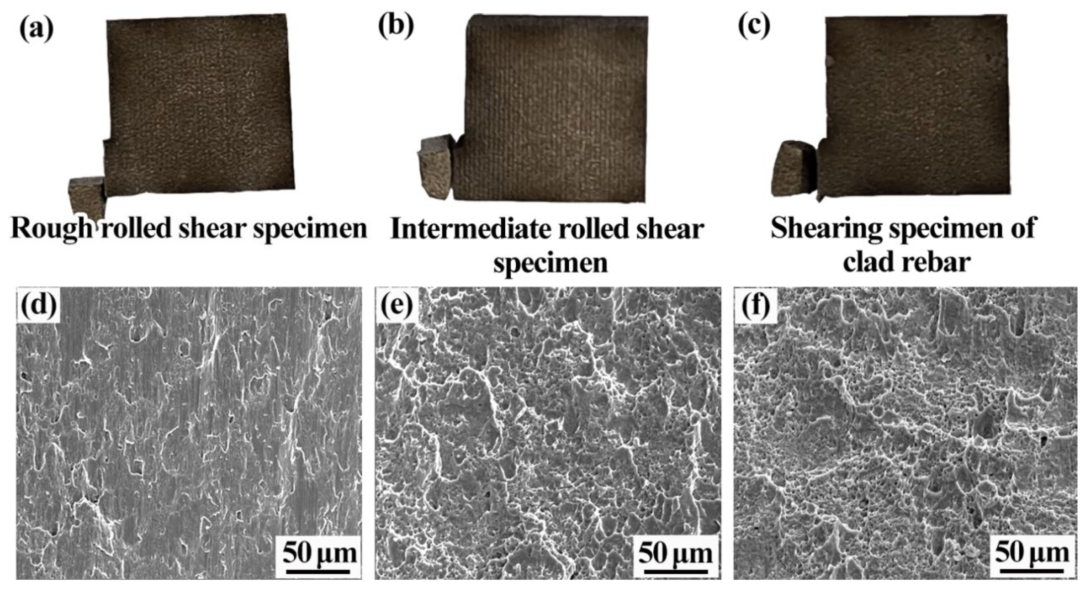
Figure 6 shows a schematic of the shearing jig during operation. First, the shear specimen was cut into the shape as shown in
Figure 7, then the shear specimen was placed in the shear jig and the cladding of the specimen was sheared from the substrate using a trapezoidal slider. Finally, the bond strength of the composite interface was calculated on the basis of the shearing forces.
Figure 8 shows a schematic of the tensile test procedure. First, the tensile specimens of specific shapes (as shown in
Figure 9) were cut using a wire cutter, and then the electro-hydraulic servo tester (Instron Limited, High Wycombe, UK) was used to test the performance of these tensile specimens.
Figure 8 shows the dimensions of the tensile specimens (unit, mm) and
Figure 9 shows a schematic of the tensile test procedure.
The tensile and shear fracture morphologies of the specimens were observed using a scanning electron microscope (Tescan Brno, South Moravia, Czech Republic) at an accelerating voltage of 30 kv.


