Figure 1.
The curve of water saturation with stages in water saturation trend: variation of saturation of the three concrete types (MIX 1, 2 and 3) in linear time scale.
Figure 1.
The curve of water saturation with stages in water saturation trend: variation of saturation of the three concrete types (MIX 1, 2 and 3) in linear time scale.
Figure 2.
Test setup for ultrasonic pulse velocity measurements.
Figure 2.
Test setup for ultrasonic pulse velocity measurements.
Figure 3.
Typical time signals of ultrasonic pulse waves propagating through the MIX 1 concrete cylinders with various water saturation conditions: (a) P-wave and (b) S-wave signals.
Figure 3.
Typical time signals of ultrasonic pulse waves propagating through the MIX 1 concrete cylinders with various water saturation conditions: (a) P-wave and (b) S-wave signals.
Figure 4.
Test setup of electrical resistivity measurements of concrete: (
a) four-point Wenner probe configuration, with an equal distance (=38 mm) between the electrodes, and (
b) A-A section view of the Wenner probe configuration in
Figure 4a.
Figure 4.
Test setup of electrical resistivity measurements of concrete: (
a) four-point Wenner probe configuration, with an equal distance (=38 mm) between the electrodes, and (
b) A-A section view of the Wenner probe configuration in
Figure 4a.
Figure 5.
Test setup for the uniaxial compressive test for measurements of compressive strength and static modulus of elasticity of concrete cylinders.
Figure 5.
Test setup for the uniaxial compressive test for measurements of compressive strength and static modulus of elasticity of concrete cylinders.
Figure 6.
Schematic diagram for the ANN architecture used in analysis: this specific architecture considers the combination of five parameters for strength estimation.
Figure 6.
Schematic diagram for the ANN architecture used in analysis: this specific architecture considers the combination of five parameters for strength estimation.
Figure 7.
Methodology flowchart for using the regression learner application inside MATLAB.
Figure 7.
Methodology flowchart for using the regression learner application inside MATLAB.
Figure 8.
Correlation between actual fc,test and predicted fc,pred using different combinations of the five parameters from multivariate regression analysis: (a) only UPV parameters: P, S, or P and S, (b) combination of UPV and one other parameter: P and WB, S and WB, P and ER, or S and ER, (c) combination of UPV, ER and WB: P, ER and WB, or S, ER and WB and (d) five all parameters: P, S, ER, D and WB. Note—S: S-wave velocity, P: P-wave velocity, ER: electric resistivity, D: density and WB: water-to-binder ratio.
Figure 9.
Correlation between actual fc,test and predicted fc,pred using different combinations of the five parameters from ANN analysis. (a) only UPV parameters: P, S, or P and S, (b) combination of UPV and one other parameter: P and WB, S and WB, P and ER or S and ER, (c) combination of UPV, ER and WB: P, ER and WB or S, ER and WB and (d) five all parameters: P, S, ER, D and WB. Note—S is S-wave velocity, P is P-wave velocity, ER is electric resistivity, D is density and WB is water-to-binder ratio.
Figure 10.
Sample parameter optimization using LM algorithm training: (a) 2 parameters, (b) 3 parameters and (c) 5 parameters.
Figure 10.
Sample parameter optimization using LM algorithm training: (a) 2 parameters, (b) 3 parameters and (c) 5 parameters.
Figure 11.
Correlation between actual fc,test and predicted fc,pred using different combinations of the five parameters from support vector machine analysis. (a) only UPV parameters: P, S, or P and S, (b) combination of UPV and one other parameter: P and WB, S and WB, P and ER or S and ER, (c) combination of UPV, ER and WB: P, ER and WB or S, ER and WB and (d) five all parameters: P, S, ER, D and WB. Note S is S-wave velocity, P is P-wave velocity, ER is electric resistivity, D is density and WB is water-to-binder ratio.
Figure 12.
Correlation between actual fc,test and predicted fc,pred using different combinations of the five parameters from Gaussian process regression analysis. (a) only UPV parameters: P, S, or P and S, (b) combination of UPV and one other parameter: P and WB, S and WB, P and ER or S and ER, (c) combination of UPV, ER and WB: P, ER and WB or S, ER and WB and (d) five all parameters: P, S, ER, D and WB. Note S is S-wave velocity, P is P-wave velocity, ER is electric resistivity, D is density and WB is water-to-binder ratio.
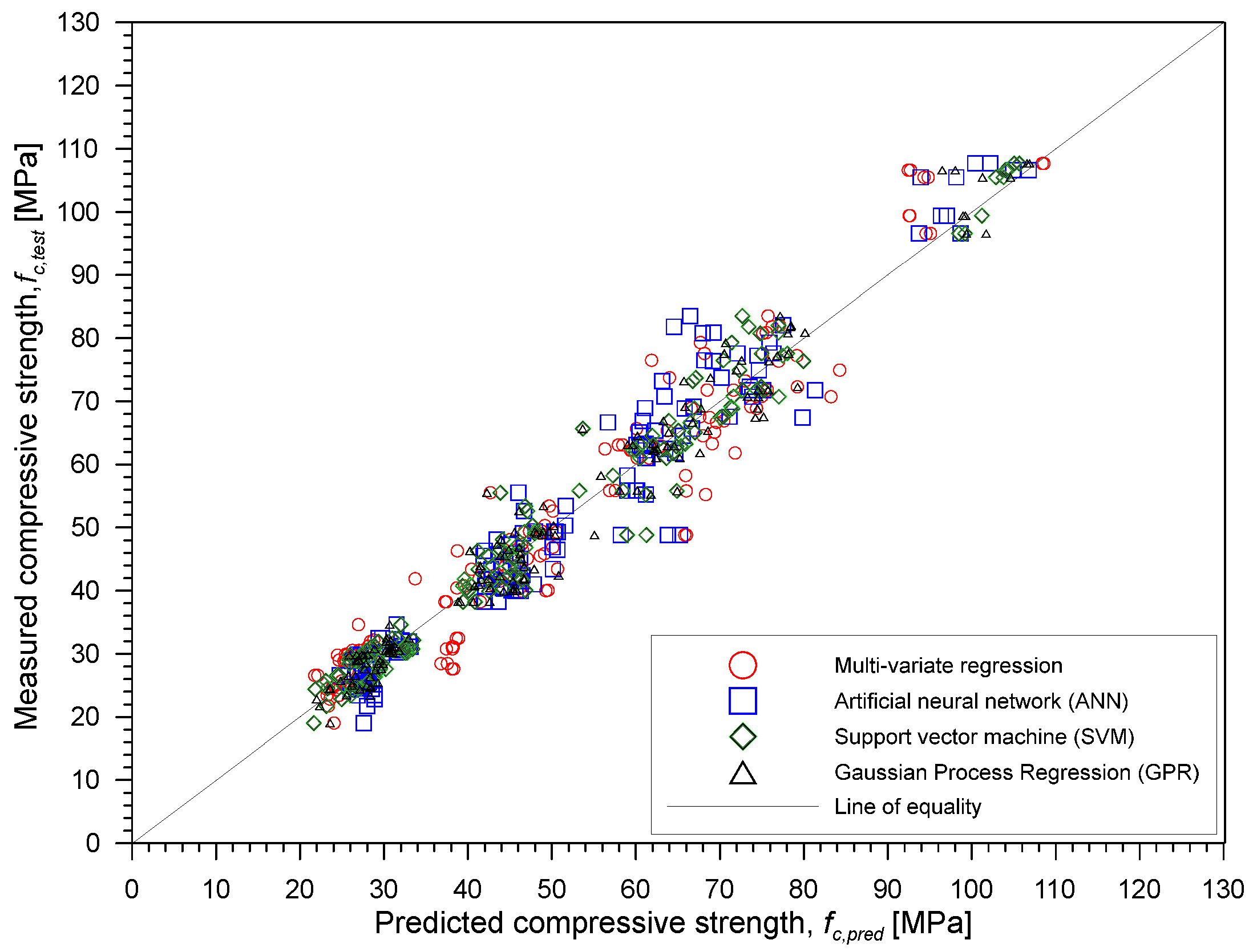
Figure 13.
Correlation between measured and predicted compressive strength of concrete using the combination of five parameters from four different machine learning methods.
Figure 13.
Correlation between measured and predicted compressive strength of concrete using the combination of five parameters from four different machine learning methods.
Table 1.
Summary of principles, advantages and limitations of popular data fusion methods in prior studies.
Table 1.
Summary of principles, advantages and limitations of popular data fusion methods in prior studies.
| Data Fusion Method | Principles | Advantage | Limitations |
|---|
| Conventional Method | 1. Regression Analysis | Conventional statistical approach in determining the relationship between a dependent variable and independent variable/s. | | |
| Machine Learning Method | 2. Artificial Neural Network (ANN) | Computing technique designed to simulate the human brain’s method in problem-solving. | Information such is stored on the entire network, not on a database. Disappearance of a few pieces of information in one place does not prevent the network from functioning.
| |
| 3. Support Vector Machine (SVM) | Classifies the data using hyperplane which acts like a decision boundary between different classes. | | |
| 4. Gaussian Process Regression (GPR) | Nonparametric, Gaussian process calculates the probability distribution over all admissible functions that fit the data set. | | |
Table 2.
Concrete mixture proportions of the concrete cylinders used in this study.
Table 2.
Concrete mixture proportions of the concrete cylinders used in this study.
| | Mixture Proportion (kg/m3) | | |
|---|
| W | C | S | G | SCMs | CA | W/B
(%) | SV/AV |
|---|
| FA | SC | AE | | |
|---|
| MIX 1 | 170 | 99 | 884 | 931 | 33 | 198 | 1.98 | 51.52 | 0.490 |
| MIX 2 | 170 | 110 | 858 | 923 | 37 | 220 | 2.57 | 35.43 | 0.495 |
| MIX 3 | 160 | 312 | 725 | 876 | 63 | 250 | 6.88 | 25.60 | 0.456 |
Table 3.
Summary of constant coefficients for the estimated saturation curves determined by non-linear regression analysis.
Table 3.
Summary of constant coefficients for the estimated saturation curves determined by non-linear regression analysis.
| | | | | | |
|---|
| MIX 1 | 9.985 × 10 | 4.312 × 10⁴ | 1.617 × 10² | 5.509 × 10² | 6.767 × 10³ |
| MIX 2 | 9.987 × 10 | 2.245 × 10⁴ | 5.738 × 10 | 3.719 × 10² | 4.788 × 10³ |
| MIX 3 | 9.900 × 10 | 2.356 × 10⁴ | 1.314 × 10² | 3.575 × 10² | 4.902 × 10³ |
Table 4.
Summary of approximate time t for the target saturation degree of specimens (25%, 50%, 75% and 100%) determined from the estimated saturation curves for the MIX 1, 2 and 3 concrete cylinders.
Table 4.
Summary of approximate time t for the target saturation degree of specimens (25%, 50%, 75% and 100%) determined from the estimated saturation curves for the MIX 1, 2 and 3 concrete cylinders.
| | Time t (min) |
|---|
| 25% | 50% | 75% | 100% |
|---|
| MIX 1 | 5.6 | 20.4 | 111.2 | 14,400 |
| MIX 2 | 8.7 | 40.7 | 271.9 | 14,400 |
| MIX 3 | 8.1 | 33.4 | 208.8 | 14,400 |
Table 5.
Summary of statistical analysis of the parameters.
Table 5.
Summary of statistical analysis of the parameters.
| | | D | S | P | ER | fc |
|---|
| Mix 1 | N | 50 | 50 | 50 | 40 | 50 |
| µ | 2089.94 | 1967.07 | 3665.97 | 49.17 | 28.01 |
| σ | 65.26 | 28.09 | 234.26 | 75.31 | 3.24 |
| COV | 3.12 | 1.43 | 6.39 | 153.16 | 11.55 |
| Mix 2 | N | 50 | 50 | 50 | 40 | 50 |
| µ | 2266.98 | 2190.95 | 4268.88 | 46.60 | 47.80 |
| σ | 46.62 | 47.54 | 246.37 | 47.51 | 7.88 |
| COV | 2.06 | 2.17 | 5.77 | 101.96 | 16.48 |
| Mix 3 | N | 50 | 49 | 50 | 40 | 48 |
| µ | 2341.04 | 2325.08 | 4581.52 | 43.94 | 74.61 |
| σ | 35.85 | 41.67 | 217.98 | 37.33 | 15.09 |
| COV | 1.53 | 1.79 | 4.76 | 84.96 | 20.22 |
Table 6.
Pearson correlation between the variables.
Table 6.
Pearson correlation between the variables.
| | WB | S | D | P | ER | SD | SAL | fc |
|---|
| WB | 1 | −0.964 | −0.899 | −0.854 | 0.000 | 0 | 0 | −0.859 |
| S | −0.964 | 1 | 0.86 | 0.8 | 0.073 | −0.057 | −0.007 | 0.874 |
| D | −0.899 | 0.86 | 1 | 0.919 | −0.25 | 0.378 | 0.041 | 0.648 |
| P | −0.854 | 0.8 | 0.919 | 1 | −0.308 | 0.386 | −0.096 | 0.582 |
| ER | 0.000 | 0.073 | −0.25 | −0.308 | 1 | −0.707 | 0 | 0.319 |
| SD | 0 | 0.378 | −0.057 | 0.386 | −0.707 | 1 | 0 | 0.022 |
| SAL | 0 | 0.041 | −0.007 | −0.096 | 0 | 0 | 1 | −0.344 |
| fc | −0.859 | 0.874 | 0.648 | 0.582 | 0.319 | −0.344 | 0.022 | 1 |
Table 7.
Summary of nonlinear equations obtained from different parameter combinations.
Table 7.
Summary of nonlinear equations obtained from different parameter combinations.
| Combination | Equation | R2 |
|---|
| P, S, WB, ER, D | | 0.930 |
| P, WB, ER | | 0.920 |
| S, WB, ER | | 0.907 |
| P, WB | | 0.886 |
| S, WB | | 0.844 |
| P, ER | | 0.118 |
| S, ER | | 0.861 |
| P, S | | 0.818 |
| P | | 0.440 |
| S | | 0.838 |
Table 8.
Coefficient of determination values (R-squared values, R2) of training results from artificial neural network (ANN) training for all experimental data.
Table 8.
Coefficient of determination values (R-squared values, R2) of training results from artificial neural network (ANN) training for all experimental data.
| Coefficient of Determination, R2 |
|---|
| Combination | Training | Validation | Test | Overall |
|---|
| S, P, WB, ER, D | 0.98 | 0.98 | 0.98 | 0.97 |
| P, WB, ER | 0.97 | 0.98 | 0.96 | 0.96 |
| S, WB, ER | 0.95 | 0.97 | 0.95 | 0.94 |
| P, WB | 0.94 | 0.98 | 0.96 | 0.93 |
| S, WB | 0.91 | 0.93 | 0.93 | 0.89 |
| P, ER | 0.77 | 0.92 | 0.84 | 0.75 |
| S, ER | 0.94 | 0.93 | 0.92 | 0.92 |
| S, P | 0.93 | 0.95 | 0.94 | 0.92 |
Table 9.
Coefficient of determination values (R-squared values, R2) of training results from regression learner training.
Table 9.
Coefficient of determination values (R-squared values, R2) of training results from regression learner training.
| Coefficient of Determination, R2 |
|---|
| Combination | SVM | GPR |
|---|
| R2 | Kernel | R2 | Model |
|---|
| S, P, WB, ER, D | 0.95 | Quadratic | 0.96 | Exponential |
| P, WB, ER | 0.94 | Quadratic | 0.94 | Exponential |
| S, WB, ER | 0.93 | Quadratic | 0.93 | Exponential |
| P, WB | 0.92 | Medium Gaussian | 0.92 | Exponential |
| S, WB | 0.85 | Fine Gaussian | 0.88 | Exponential |
| P, ER | 0.71 | Fine Gaussian | 0.70 | Exponential |
| S, ER | 0.86 | Medium Gaussian | 0.90 | Exponential |
| S, P | 0.88 | Fine Gaussian | 0.92 | Exponential |
| P | 0.35 | Cubic | 0.34 | Exponential |
| S | 0.84 | Fine Gaussian | 0.86 | Exponential |
Table 10.
R-squared comparison between the different methods used in the study.
Table 10.
R-squared comparison between the different methods used in the study.
| R-Squared |
|---|
| Combination | ANN | SVM | GPR | Multi-Variate Regression |
|---|
| S, P, WB, ER, D | 0.97 | 0.95 | 0.96 | 0.93 |
| S, WB | 0.89 | 0.83 | 0.85 | 0.84 |
| S, WB, ER | 0.94 | 0.93 | 0.93 | 0.91 |
| P, WB | 0.93 | 0.92 | 0.92 | 0.89 |
| P, WB, ER | 0.96 | 0.94 | 0.94 | 0.92 |
| S | - | 0.84 | 0.86 | 0.84 |
| P | - | 0.35 | 0.34 | 0.44 |
| S, P | 0.92 | 0.88 | 0.92 | 0.82 |
| S, ER | 0.92 | 0.86 | 0.90 | 0.86 |
| P, ER | 0.75 | 0.71 | 0.70 | 0.12 |
Table 11.
Comparison of RMSE between the different methods used in the study.
Table 11.
Comparison of RMSE between the different methods used in the study.
| RMSE (MPa) |
|---|
| Combination | ANN | SVM | GPR | Multi-Variate Regression |
|---|
| S, P, WB, ER, D | 4.988 | 4.971 | 4.292 | 5.879 |
| S, WB | 8.354 | 8.762 | 7.783 | 8.783 |
| S, WB, ER | 6.153 | 5.991 | 5.742 | 6.796 |
| P, WB | 9.476 | 6.476 | 6.163 | 7.522 |
| P, WB, ER | 5.493 | 5.485 | 5.305 | 6.4792 |
| S | - | 9.146 | 8.462 | 9.769 |
| P | - | 18.04 | 18.154 | 18.708 |
| S, P | 7.055 | 7.843 | 6.543 | 9.512 |
| S, ER | 6.745 | 8.2987 | 7.0455 | 8.293 |
| P, ER | 11.950 | 12.036 | 12.305 | 20.896 |
Table 12.
Comparison of MAE between the different methods used in the study.
Table 12.
Comparison of MAE between the different methods used in the study.
| MAE (MPa) |
|---|
| Combination | ANN | SVM | GPR | Multi-Variate Regression |
|---|
| S, P, WB, ER, D | 3.579 | 3.568 | 3.058 | 4.4005 |
| S, WB | 6.291 | 6.230 | 5.741 | 6.297 |
| S, WB, ER | 4.551 | 4.374 | 4.240 | 5.190 |
| P, WB | 7.073 | 4.963 | 4.698 | 5.849 |
| P, WB, ER | 3.929 | 3.975 | 3.918 | 5.161 |
| S | - | 6.367 | 6.141 | 7.059 |
| P | - | 12.337 | 13.072 | 12.756 |
| S, P | 5.235 | 5.638 | 4.447 | 6.918 |
| S, ER | 5.005 | 6.035 | 5.121 | 6.577 |
| P, ER | 9.414 | 8.419 | 9.081 | 17.215 |


