
Crack Initiation Mechanism and Life Prediction of Ti60 Titanium Alloy Considering Stress Ratios Effect in Very High Cycle Fatigue Regime

 , ,
, , 
Abstract
:1. Introduction
2. Experimental Procedure
2.1. Material
2.2. Experiment
3. Experimental Results
3.1. S-N Diagram
3.2. Fracture Surfaces
4. The Effect of the Stress Ratio on the Production of Fatigue Failure
5. Fatigue Strength Prediction
6. Fatigue Life Prediction of Internal Crack Initiation
7. Conclusions and Perspectives
7.1. Conclusions
- (1)
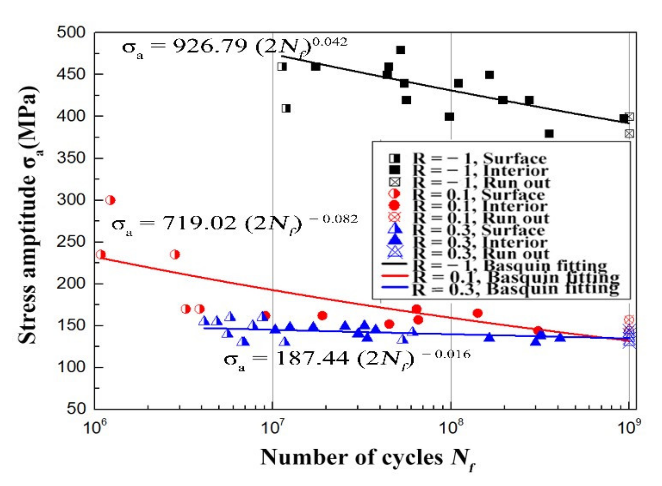
- The S-N curves with different stress ratios show continuous declining tendencies. Fatigue cracks found to be initiated from subsurface of the specimens, and the tendency of internal crack initiation increases when R > 0.
- (2)
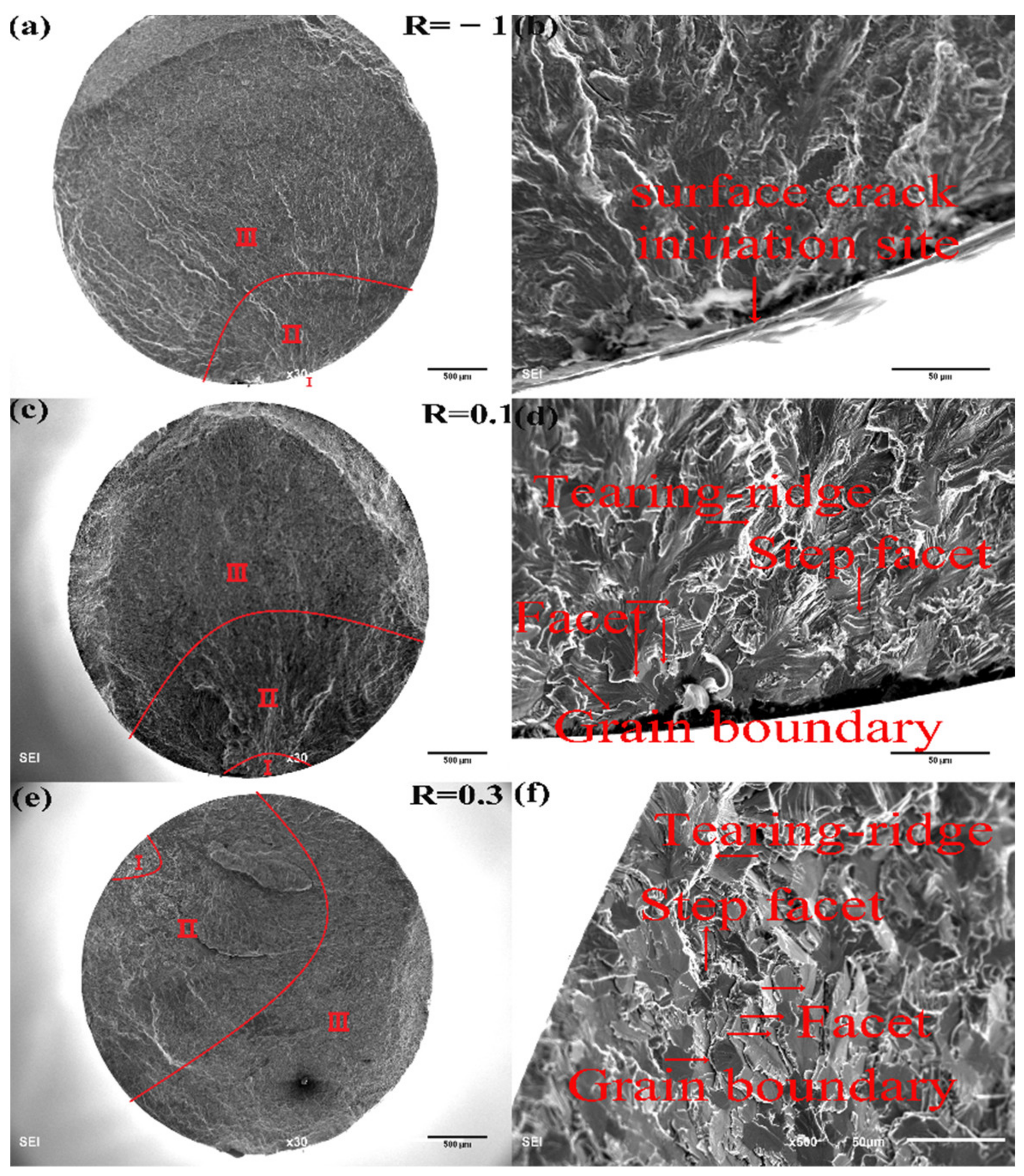
- Based on SEM observations on fracture surfaces, the whole progress of fatigue failure can be divided into four regions: (I) crack initiating stage involving a large number of small flat rough areas; (II) highly rough areas containing radial ridges; (III) a relatively flat and wide area containing radial stripes; and (IV) an area containing obvious dimples.
- (3)
- The ΔKI of internal crack initiation is much larger than that of surface crack initiation. The mean values of ΔKI are 4.36, 3.57 and 3.49 MPa at stress ratios of −1, 0.1 and 0.3, respectively. The difference in the ΔKI can be explained by the crack closure effect.
- (4)
- Two modified fatigue strength prediction models on the Ti60 titanium alloy are developed and in good agreement with experimental results.
7.2. Perspectives
- (1)
- The very high cycle fatigue regime for Ti60 titanium alloy at high temperature especially at 600 °C need to be researched for its the service environment of Ti60 titanium.
- (2)
- The temperature with stress ratio effect on Ti60 titanium alloy at a very high cycle regime also need to be researched, the comprehensive influence factor for a very high cycle regime should be further researched.
Author Contributions
Funding
Institutional Review Board Statement
Informed Consent Statement
Data Availability Statement
Conflicts of Interest
References
- Rockel, M.B.; Roman, B. Titanium and Titanium Alloys. Corrosion Handbook; Dechema: Frankfurt, Germany, 2012; Volume 43, pp. 24–29. [Google Scholar]
- He, Y.; Xiao, G.; Li, W.; Huang, Y. Residual Stress of a TC17 Titanium Alloy after Belt Grinding and Its Impact on the Fatigue Life. Materials 2018, 11, 2218. [Google Scholar] [CrossRef] [PubMed] [Green Version]
- Fang, C.D. High cycle fatigue research program of aircraft gas turbine engine. Int. Aviat. 2005, 8, 63–65. [Google Scholar]
- Bathias, C. There is no infinite fatigue life in metallic materials. Fatigue Fract. Eng. Mater. Struct. 1999, 22, 559–565. [Google Scholar] [CrossRef]
- Heinz, S.; Balle, F.; Wagner, G.D.; Eifler, D. Analysis of fatigue properties and failure mechanisms of Ti6Al4V in the very high cycle fatigue regime using ultrasonic technology and 3D laser scanning vibrometry. Ultrasonics 2013, 53, 1433–1440. [Google Scholar] [CrossRef] [PubMed]
- Liu, X.; Sun, C.; Hong, Y. Effects of stress ratio on high-cycle and very-high-cycle fatigue behavior of a Ti-6Al-4V alloy. Mater. Sci. Eng. A 2015, 622, 228–235. [Google Scholar] [CrossRef]
- Li, W.; Zhao, H.; Nehila, A.; Zhang, Z.; Sakai, T. Very high cycle fatigue of TC4 titanium alloy under variable stress ratio: Failure mechanism and life prediction. Int. J. Fatigue 2017, 104, 342–354. [Google Scholar] [CrossRef]
- Heinz, S.; Eifler, D. Crack initiation mechanisms of Ti6A14V in the very high cycle fatigue regime. Int. J. Fatigue 2016, 93, 301–308. [Google Scholar] [CrossRef]
- Chai, G. The formation of subsurface non-defect fatigue crack origins. Int. J. Fatigue 2006, 28, 1533–1539. [Google Scholar] [CrossRef]
- Jha, S.K.; Szczepanski, C.J.; John, R.; Larsen, J.M. Deformation heterogeneities and their role in life-limiting fatigue failures in a two-phase titanium alloy. Acta Mater. 2015, 82, 378–395. [Google Scholar] [CrossRef]
- Larsen, J.; Jha, S.; Szczepanski, C.; Caton, M.; John, R.; Rosenberger, A.; Buchanan, D.; Golden, P.; Jira, J. Reducing uncertainty in fatigue life limits of turbine engine alloys. Int. J. Fatigue 2013, 57, 103–112. [Google Scholar] [CrossRef] [Green Version]
- Jha, S.K.; Szczepanski, C.J.; Golden, P.J.; Porter, W.J., III; John, R. Characterization of fatigue crack-initiation facets in relation to lifetime variability in Ti-6Al-4V. Int. J. Fatigue 2012, 42, 248–257. [Google Scholar] [CrossRef]
- Golden, P.J.; John, R.; Porter, W.J., III. Investigation of variability in fatigue crack nucleation and propagation in alpha+beta Ti-6Al-4V. In Proceedings of the 10th International Fatigue Conference, Prague, Czech Republic, 6–11 June 2010; pp. 1839–1847. [Google Scholar]
- Jha, S.; Larsen, J.; Rosenberger, A. Rosenberger, Towards a physics-based description of fatigue variability behavior in probabilistic life-prediction. Eng. Fract. Mech. 2009, 76, 681–694. [Google Scholar] [CrossRef]
- He, C.; Liu, Y.; Dong, J.; Wang, Q.; Wagner, D.; Bathias, C. Through thickness property variations in friction stir welded AA6061 joint fatigued in very high cycle fatigue regime. Int. J. Fatigue 2016, 82, 379–386. [Google Scholar] [CrossRef]
- Hong, Y.; Lei, Z.; Sun, C.; Zhao, A. Propensities of crack interior initiation and early growth for very-high-cycle fatigue of high strength steels. Int. J. Fatigue 2014, 58, 144–151. [Google Scholar] [CrossRef] [Green Version]
- Wang, Q.Y.; Bathias, C.; Kawagoishi, N.; Chen, Q. Effect of inclusion on subsurface crack initiation and gigacycle fatigue strength. Int. J. Fatigue 2002, 24, 1269–1274. [Google Scholar] [CrossRef]
- Cui, W.; Chen, X.; Cheng, L.; Ding, J.; Wang, C.; Wang, B. Fatigue property and failure mechanism of TC4 titanium alloy in the HCF and VHCF region considering different forging processes. Mater. Res. Express 2021, 8, 046524. [Google Scholar] [CrossRef]
- Yang, K.; Zhong, B.; Huang, Q.; He, C.; Huang, Z.-Y.; Wang, Q.; Liu, Y.-J. Stress ratio and notch effects on the very high cycle fatigue properties of a near-alpha titanium alloy. Materials 2018, 11, 1778. [Google Scholar] [CrossRef] [Green Version]
- Li, W.; Xing, X.; Gao, N.; Wang, P. Subsurface crack nucleation and growth behavior and energy-based life prediction of a titanium alloy in high-cycle and very-high-cycle regimes. Eng. Fract. Mech. 2019, 221, 106705. [Google Scholar] [CrossRef]
- Es-Souni, M. Creep deformation behavior of three high-temperature near alpha-Ti alloys: IMI 834, IMI 829, and IMI 685. Metall. Mater. Trans. A 2001, 32, 285–293. [Google Scholar] [CrossRef]
- Williams, J.C.; Starke, E.A., Jr. Progress in structural materials for aerospace systems. Acta Mater. 2003, 51, 5775–5799. [Google Scholar] [CrossRef]
- Yang, L.; Liu, J.; Tan, J.; Chen, Z.; Wang, Q.; Yang, R. Dwell and normal cyclic fatigue behaviours of Ti60 alloy. J. Mater. Sci. Technol. 2014, 30, 706–709. [Google Scholar] [CrossRef]
- Peters, M.; Kumpfert, J.; Ward, C.; Leyens, C. Titanium alloys for aerospace applications. Adv. Eng. Mater. 2003, 5, 419–427. [Google Scholar] [CrossRef]
- Satyanarayana, D.; Omprakash, C.; Sridhar, T.; Kumar, V. Effect of microstructure on creep crack growth behavior of a near-alpha titanium alloy IMI-834. Metall. Mater. Trans. A 2009, 40, 128–137. [Google Scholar] [CrossRef]
- Whittaker, M.; Harrison, W.; Hurley, P.; Williams, S. Modelling the behaviour of titanium alloys at high temperature for gas turbine applications. Mater. Sci. Eng. A 2010, 527, 4365–4372. [Google Scholar] [CrossRef] [Green Version]
- Qin, Y.; Zhang, D.; Jiang, W.; He, X. Microstructure and mechanical properties of welded joints of titanium alloy Ti60 after laser welding and subsequent heat treatment. Met. Sci. Heat Treat. 2021, 62, 689–695. [Google Scholar] [CrossRef]
- Song, D.; Wang, T.; Jiang, S.; Xie, Z. Influence of welding parameters on microstructure and mechanical properties of electron beam welded Ti60 to GH3128 joint with a Cu interlayer. Chin. J. Aeronaut. 2021, 34, 39–46. [Google Scholar] [CrossRef]
- Wang, T.; Lu, S.; Wang, K.; Ouyang, D.; Yao, Q. Hot deformation behavior and processing parameter optimization of Ti60 alloy. Rare Met. Mater. Eng. 2020, 49, 3552–3561. [Google Scholar]
- Zhang, Y.; Wang, B.; Zhang, H.; Li, Y. The effects of thermal deformation temperatures on microstructure and mechanical properties of TiBw/Ti60 composites synthesized by SPS. Mater. Res. Express 2021, 8, 066520. [Google Scholar] [CrossRef]
- Huang, Z.Y.; Liu, H.Q.; Wang, H.M.; Wagner, D.; Khan, M.K.; Wang, Q.Y. Effect of stress ratio on VHCF behavior for a compressor blade titanium alloy. Int. J. Fatigue 2016, 93, 232–237. [Google Scholar] [CrossRef]
- Liu, X.; Sun, C.; Hong, Y. Faceted crack initiation characteristics for high-cycle and very-high-cycle fatigue of a titanium alloy under different stress ratios. Int. J. Fatigue 2016, 92, 434–441. [Google Scholar] [CrossRef] [Green Version]
- Gao, T.; Xue, H.; Sun, Z.; Retraint, D.; He, Y. Micromechanisms of crack initiation of a Ti-8Al-1Mo-1V alloy in the very high cycle fatigue regime. J. Int. J. Fatigue 2021, 150, 106314. [Google Scholar] [CrossRef]
- Sakai, T.; Sato, Y.; Oguma, N. Characteristic S-N properties of high-carbon-chromium-bearing steel under axial loading in long-life fatigue. Fatigue Fract. Eng. Mater. Struct. 2002, 25, 765–773. [Google Scholar] [CrossRef]
- Murakami, Y.; Nomoto, T.; Ueda, T. On the mechanism of fatigue failure in the superlong life regime (N > 10(7) cycles). Part II: A fractographic investigation. Fatigue Fract. Eng. Mater. Struct. 2000, 23, 903–910. [Google Scholar] [CrossRef]
- Sakai, T.; Sato, Y.; Nagano, Y.; Takeda, M.; Oguma, N. Effect of stress ratio on long life fatigue behavior of high carbon chromium bearing steel under axial loading. Int. J. Fatigue 2006, 28, 1547–1554. [Google Scholar] [CrossRef]
- Sohar, C.R.; Betzwar-Kotas, A.; Gierl, C.; Weiss, B.; Danninger, H. Fractographic evaluation of gigacycle fatigue crack nucleation and propagation of a high Cr alloyed cold work tool steel. Int. J. Fatigue 2008, 30, 2191–2199. [Google Scholar] [CrossRef]
- Nikitin, A.; Palin-Luc, T.; Shanyavskiy, A. Crack initiation in VHCF regime on forged titanium alloy under tensile and torsion loading modes. Int. J. Fatigue 2016, 93, 318–325. [Google Scholar] [CrossRef] [Green Version]
- Stanzl-Tschegg, S.; Schönbauer, B. Near-threshold fatigue crack propagation and internal cracks in steel. Procedia Eng. 2010, 2, 1547–1555. [Google Scholar] [CrossRef] [Green Version]
- Mayer, H.; Haydn, W.; Schuller, R.; Issler, S.; Furtner, B.; Bacher-Höchst, M. Very high cycle fatigue properties of bainitic high carbon-chromium steel. Int. J. Fatigue 2009, 31, 242–249. [Google Scholar] [CrossRef]
- Sun, C.; Liu, X.; Hong, Y. A two-parameter model to predict fatigue life of high-strength steels in a very high cycle fatigue regime. Acta Mech. Sin. 2015, 31, 383–391. [Google Scholar] [CrossRef]


| Material | Ti | Al | Sn | Zr | Mo | Si | Ta | C |
|---|---|---|---|---|---|---|---|---|
| Ti60 | 84.84 | 5.6 | 4.0 | 3.5 | 1.0 | 0.5 | 0.5 | 0.06 |
| Alloy | E/GPa | σb/Mpa | σ0.2/Mpa | A/% | Z/% |
|---|---|---|---|---|---|
| Ti60 | 114 | 1044 | 934 | 11 | 23 |
| Stress Ratio | R = −1 | R = 0.1 | R = 0.3 |
|---|---|---|---|
| a | 926.79 | 719.02 | 187.44 |
| b | −0.042 | −0.082 | −0.016 |
| Fatigue limit (MPa) | 380 | 144 | 125 |
| Stress Ratio | R = −1 | R = 0.1 | R = 0.3 (Surface) | R = 0.3 (Interior) |
|---|---|---|---|---|
| Mean value | 4.36 | 3.96 | 3.81 | 3.48 |
| standard error | 0.021 | 0.034 | 0.049 | 0.041 |
| Standard deviation | 0.073 | 0.107 | 0.148 | 0.136 |
| R | C | t |
|---|---|---|
| −1 | 1.11565 × 1050 | −7.14963 |
| 0.1 | 1.52153 × 10¹⁵ | −1.47486 |
| 0.3 | 2.21737 × 10¹⁴ | −1.42973 |
| R | α | l |
|---|---|---|
| −1 | 4.11 × 10⁻⁷ | 2.44709 |
| 0.1 | 1.32 × 10⁻¹¹ | −4.36986 |
| 0.3 | 0.0488 | 6.6042 |
Publisher’s Note: MDPI stays neutral with regard to jurisdictional claims in published maps and institutional affiliations. |
© 2022 by the authors. Licensee MDPI, Basel, Switzerland. This article is an open access article distributed under the terms and conditions of the Creative Commons Attribution (CC BY) license (https://creativecommons.org/licenses/by/4.0/).
Share and Cite
He, R.; Peng, H.; Liu, F.; Khan, M.K.; Chen, Y.; He, C.; Wang, C.; Wang, Q.; Liu, Y. Crack Initiation Mechanism and Life Prediction of Ti60 Titanium Alloy Considering Stress Ratios Effect in Very High Cycle Fatigue Regime. Materials 2022, 15, 2800. https://doi.org/10.3390/ma15082800
He R, Peng H, Liu F, Khan MK, Chen Y, He C, Wang C, Wang Q, Liu Y. Crack Initiation Mechanism and Life Prediction of Ti60 Titanium Alloy Considering Stress Ratios Effect in Very High Cycle Fatigue Regime. Materials. 2022; 15(8):2800. https://doi.org/10.3390/ma15082800
Chicago/Turabian StyleHe, Ruixiang, Haotian Peng, Fulin Liu, Muhammad Kashif Khan, Yao Chen, Chao He, Chong Wang, Qingyuan Wang, and Yongjie Liu. 2022. "Crack Initiation Mechanism and Life Prediction of Ti60 Titanium Alloy Considering Stress Ratios Effect in Very High Cycle Fatigue Regime" Materials 15, no. 8: 2800. https://doi.org/10.3390/ma15082800
APA StyleHe, R., Peng, H., Liu, F., Khan, M. K., Chen, Y., He, C., Wang, C., Wang, Q., & Liu, Y. (2022). Crack Initiation Mechanism and Life Prediction of Ti60 Titanium Alloy Considering Stress Ratios Effect in Very High Cycle Fatigue Regime. Materials, 15(8), 2800. https://doi.org/10.3390/ma15082800