Analysis of the Microstructure Development of Nb-Microalloyed Steel during Rolling on a Heavy-Section Mill
Abstract
1. Introduction
2. Microstructure Evolution Model
Description of the Microstructure Development Model Modification
- −
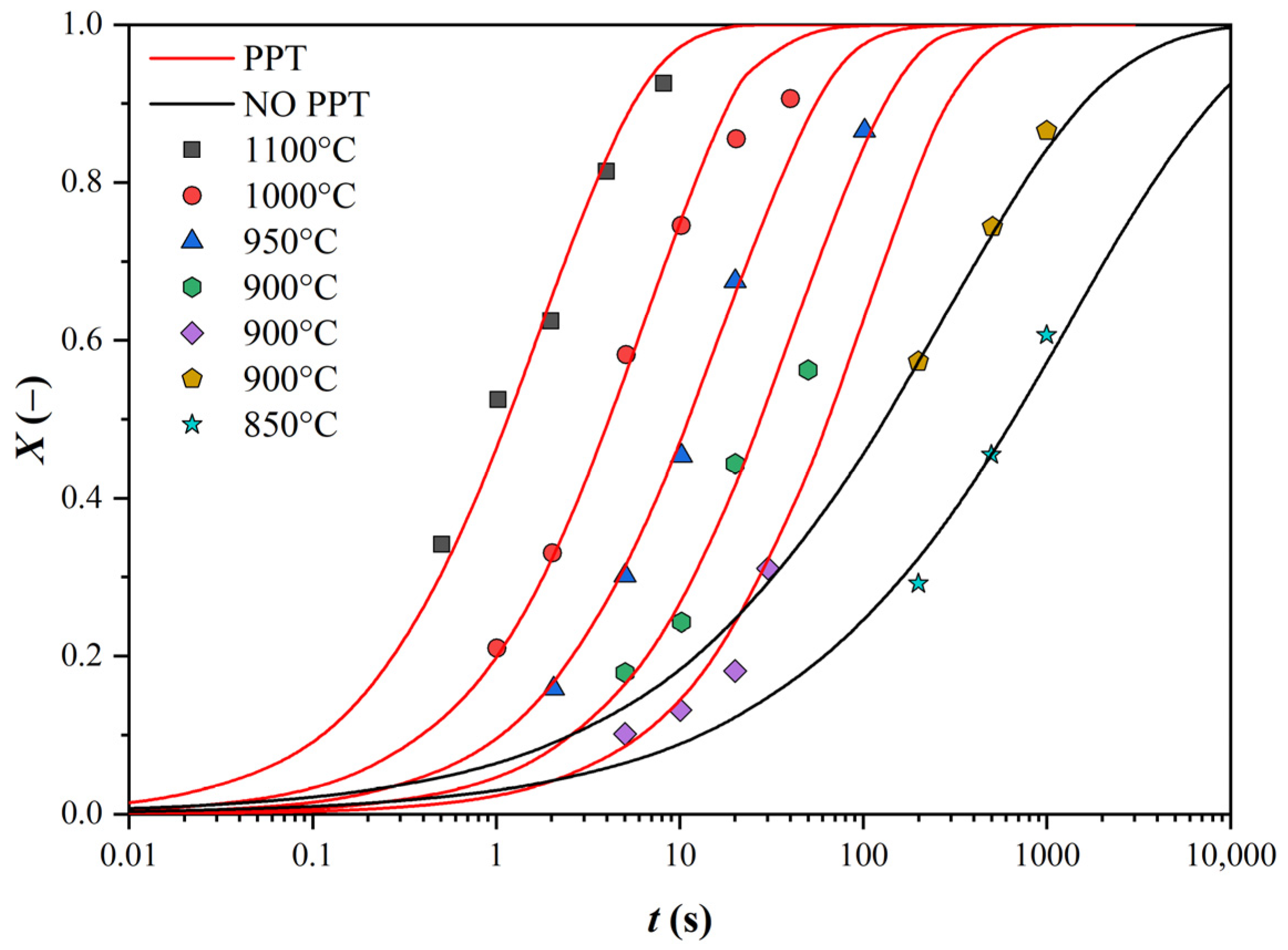
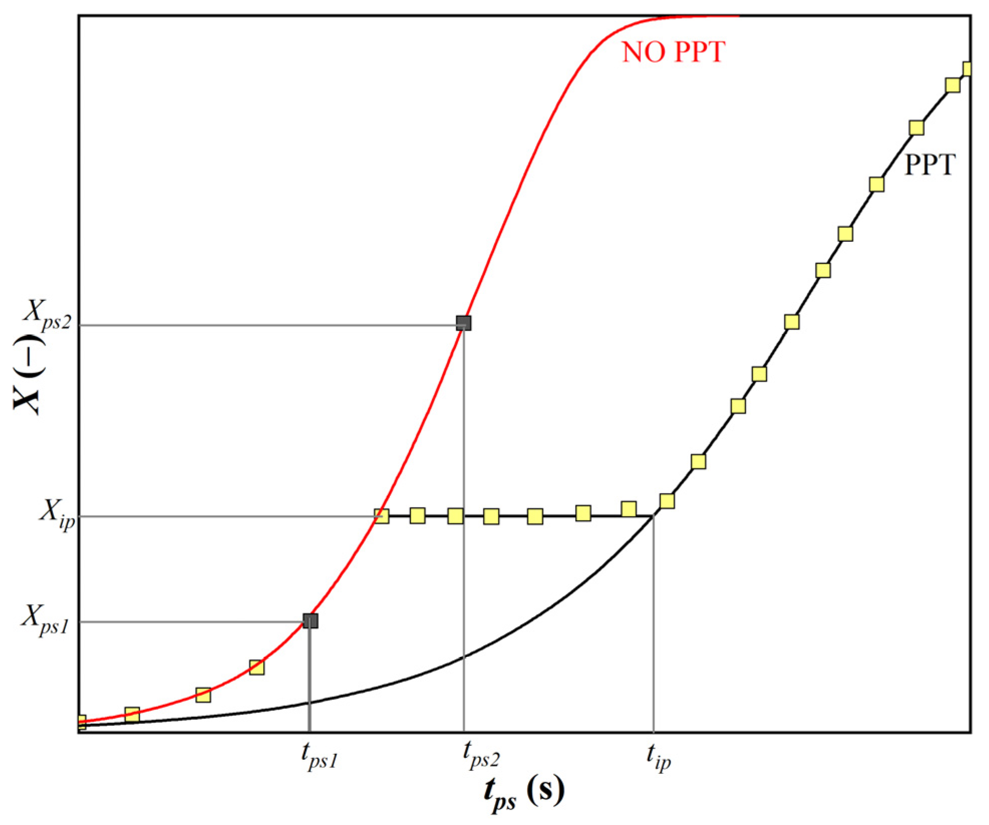
- greater than the proportion of the softened structure at time tps for the curve without SIP (tps1 and Xtps1 in Figure 9);
- −
- less than the proportion of the softened structure at time tps for the curve without SIP (tps2 and Xtps2 in Figure 9).
3. Plain Strain Compression Test (PSCT)
3.1. Experiment Description
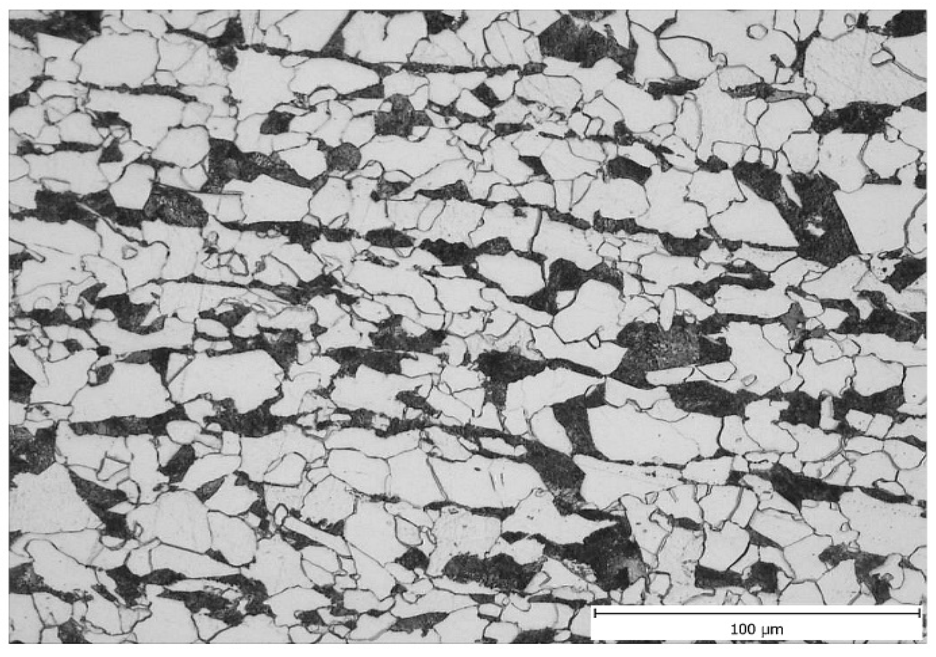
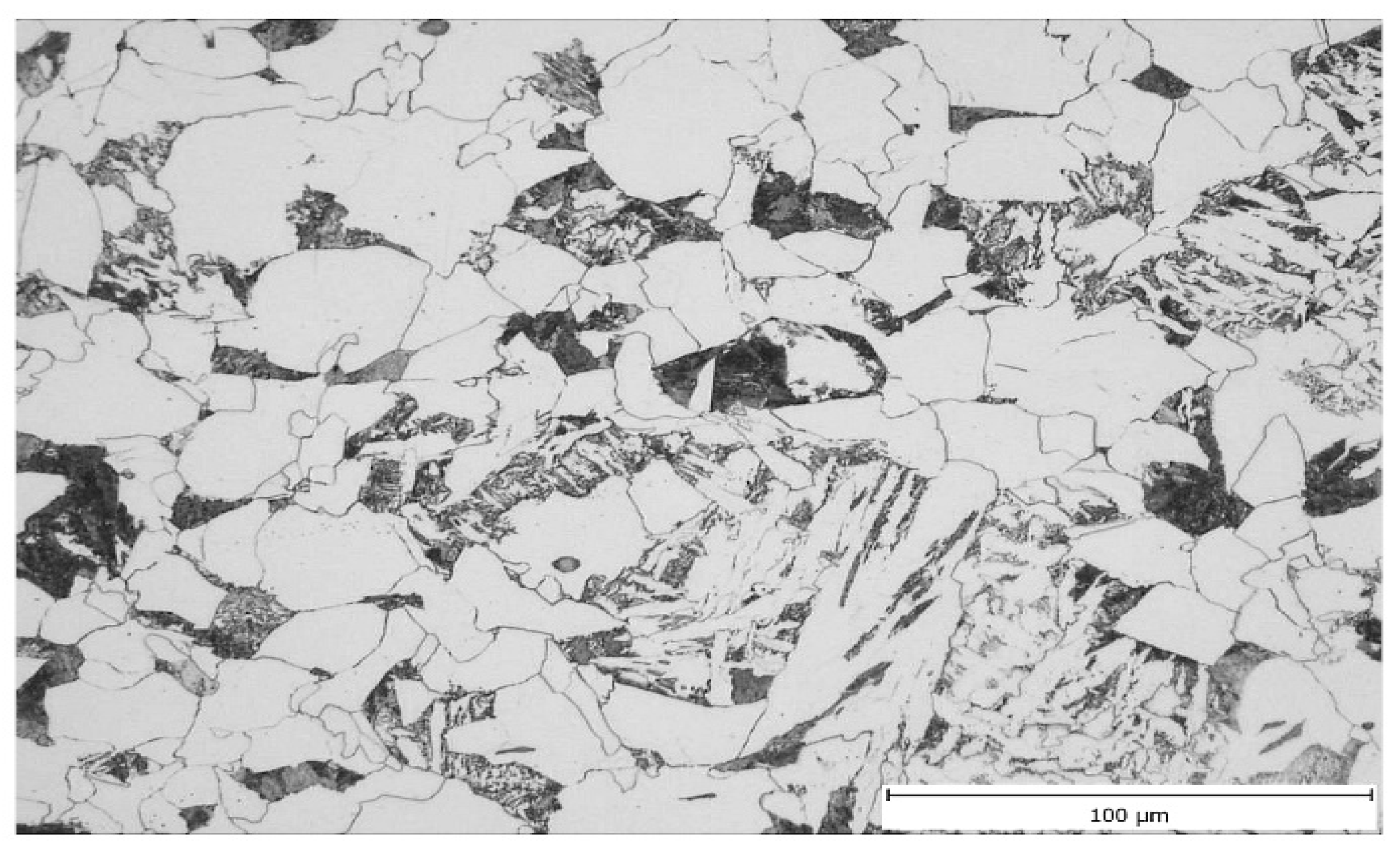
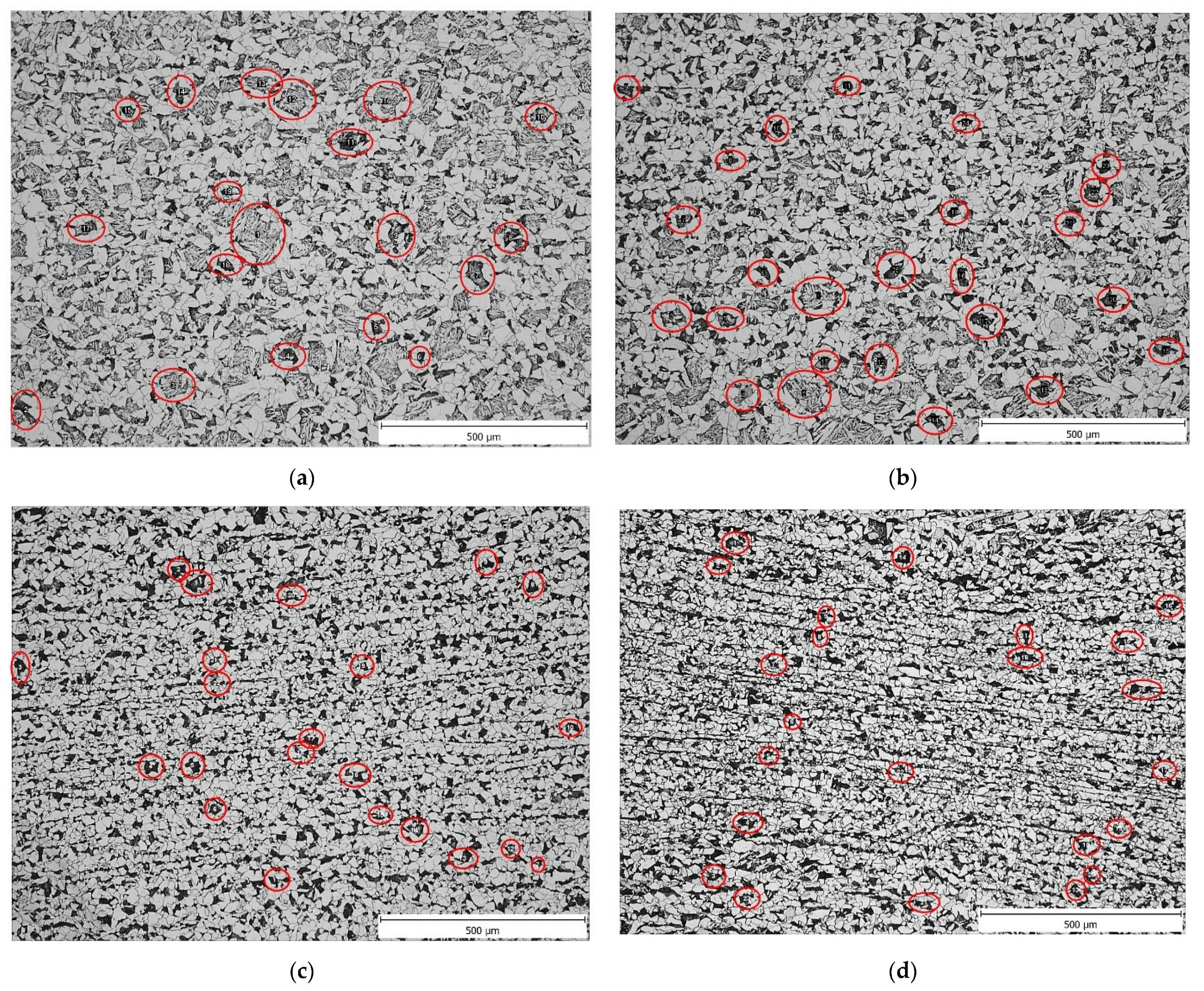
3.2. Microstructural Analysis
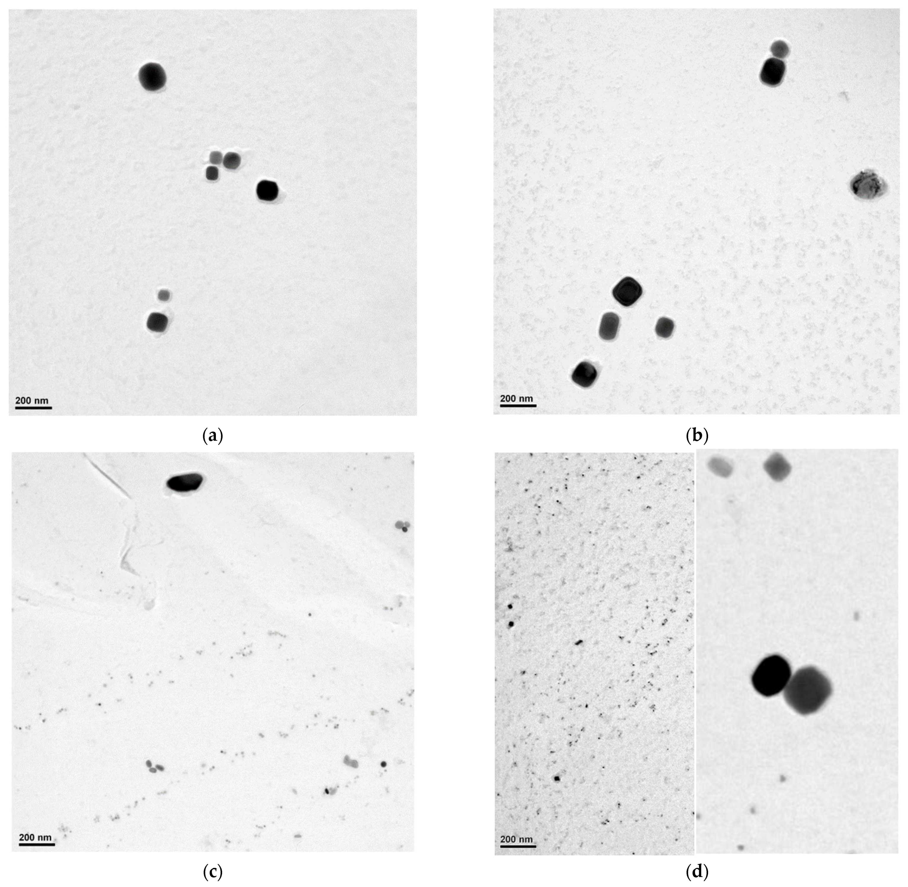
3.3. Precipitate Analysis
3.4. Simulation of PSCTs Using a Modified Microstructure Evolution Model
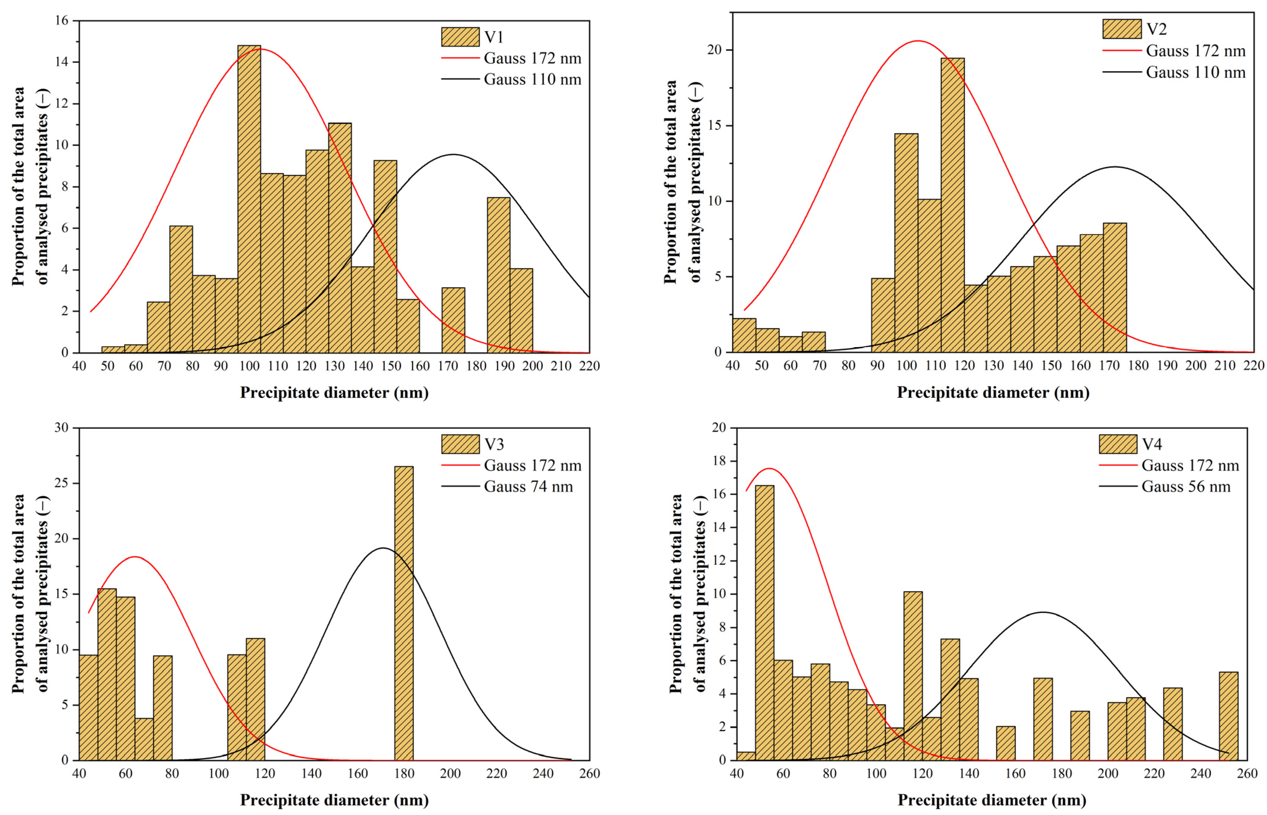
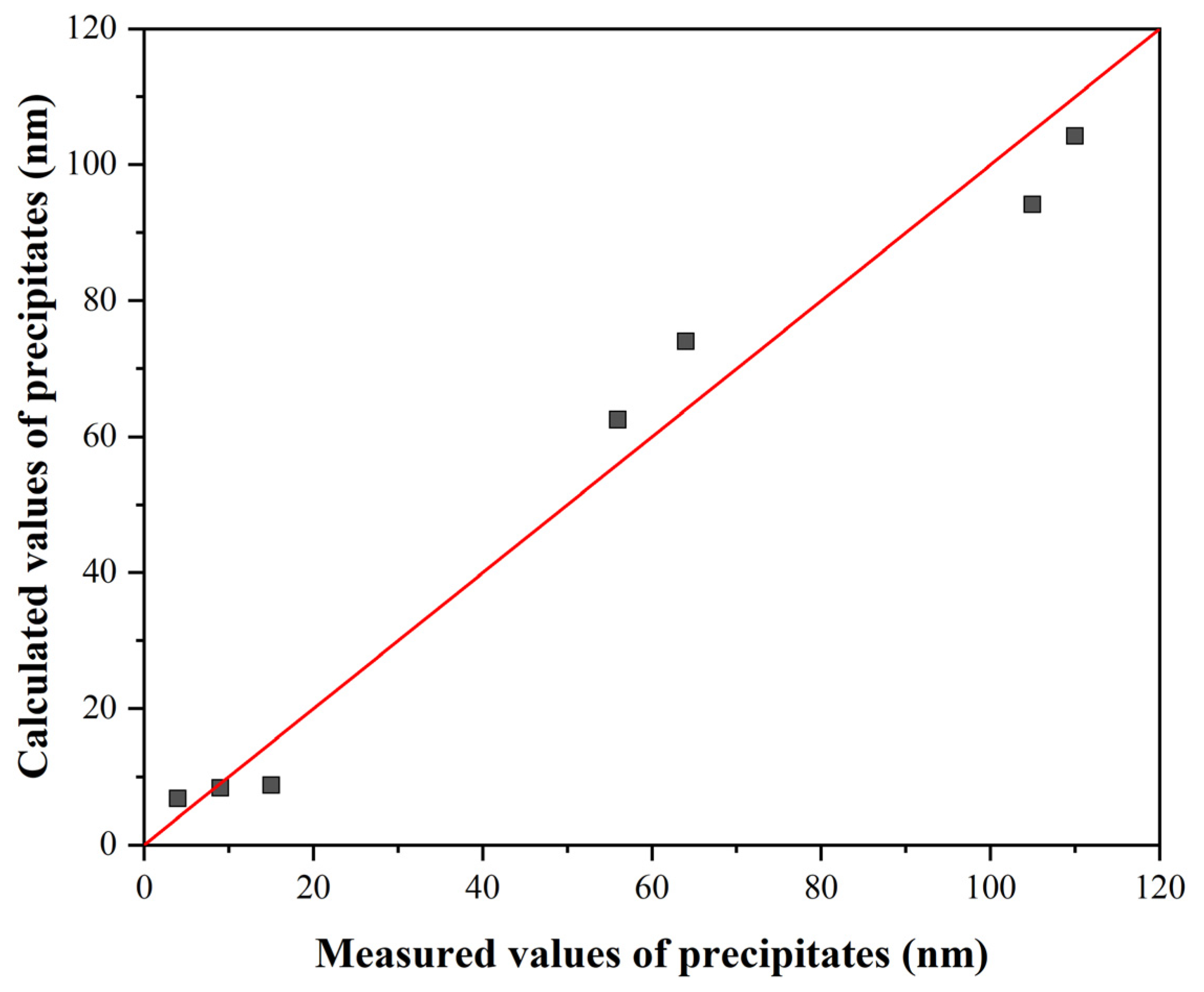
3.5. Analysis of Precipitate Size Distribution
- −
- undissolved precipitates with a mean value of 172 nm;
- −
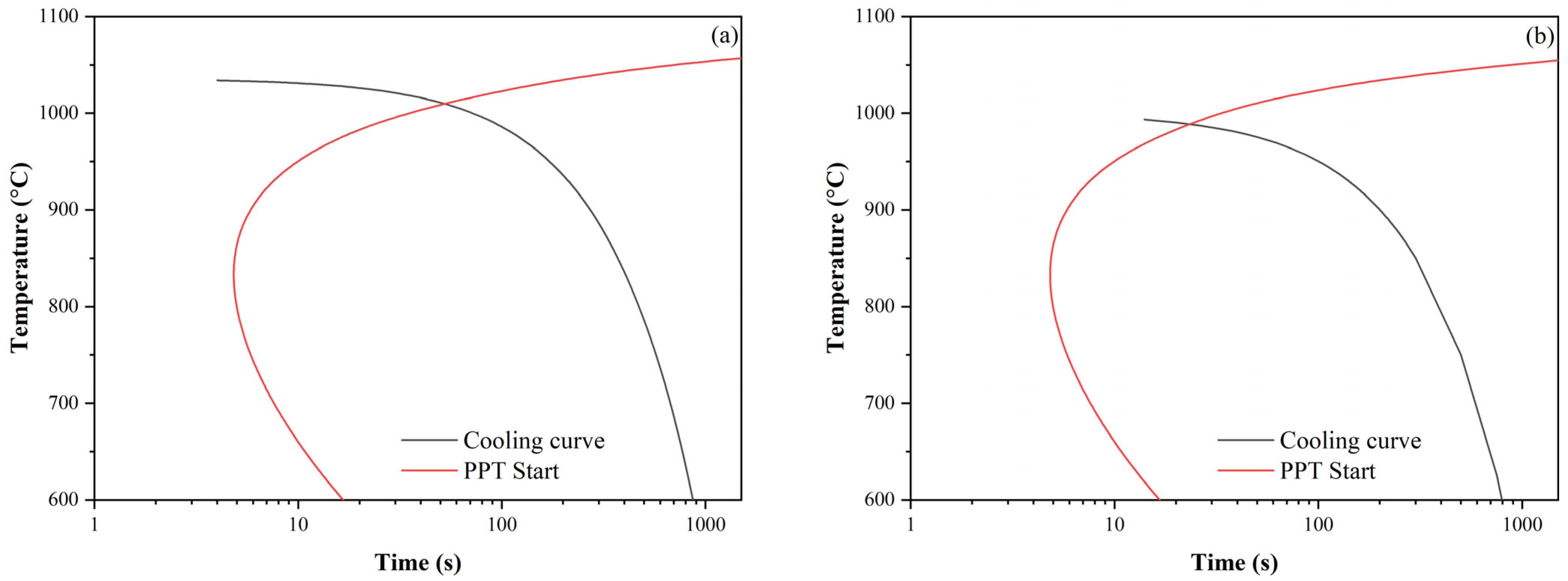
- precipitates formed during cooling after rolling with mean values for V1 and V2 of 110 and 105 nm, respectively. The lower value for V2 is due to the lower precipitation temperature (1009 °C for V1 vs. 989 °C for V2).
- −
- undissolved precipitates with a mean value of 172 nm;
- −
- precipitates formed during cooling after rolling with a mean value of 64 nm (precipitation temperature 944 °C, solid solution partially depleted of Nb due to previous precipitation);
- −
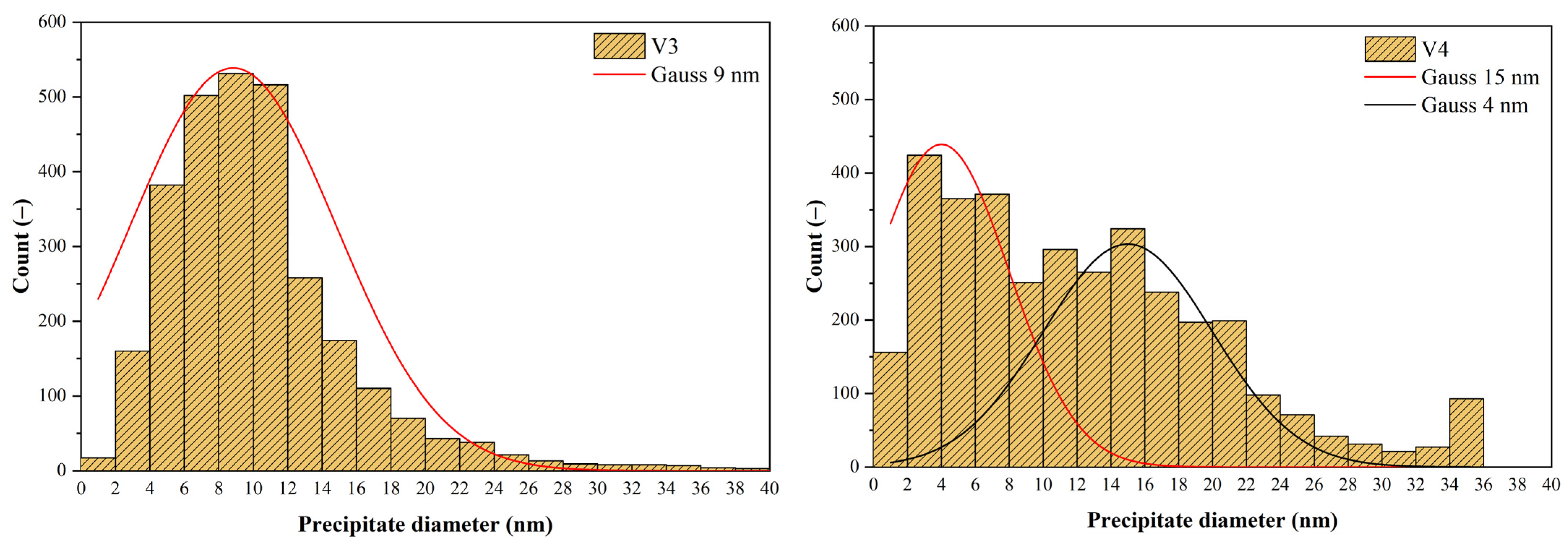
- precipitates formed during precipitation in the pause between the 6th and 7th passes; these have a mean size of only 9 nm due to the limited time for precipitation (24 s).
- −
- undissolved precipitates with a mean value of 172 nm;
- −
- precipitates formed during cooling after rolling with a mean value of 56 nm (precipitation temperature 914 °C, solid solution partially depleted of Nb due to previous precipitation);
- −
- precipitates formed during precipitation in the pause between the 6th and 7th passes; these have a mean size of 15 nm due to the limited time for precipitation (32 s);
- −
- precipitates formed during precipitation in the pause between the 5th and 6th passes; these have an average size of only 4 nm due to the limited time for precipitation (19 s).
4. Discussion
5. Conclusions
Author Contributions
Funding
Institutional Review Board Statement
Informed Consent Statement
Data Availability Statement
Acknowledgments
Conflicts of Interest
References
- Bhadeshia, H.K.D.H.; Honeycombe, R.W.K. Steels: Microstructure and Properties, 4th ed.; Butterworth-Heinemann: Amsterdam, The Netherlands, 2017; ISBN 978-0-08-100270-4. [Google Scholar]
- Mathematical and Physical Simulation of the Properties of Hot Rolled Products; Elsevier: Amsterdam, The Netherlands, 1999; ISBN 978-0-08-042701-0.
- Thermomechanical Processing of High-Strength Low-Alloy Steels; Elsevier: Amsterdam, The Netherlands, 1988; ISBN 978-0-408-11034-1.
- Verlinden, B.; Cahn, R.W. Thermo-Mechanical Processing of Metallic Materials, 1st ed.; Verlinden, B., Cahn, R.W., Eds.; Pergamon materials series; Pergamon/Elsevier: Amsterdam, The Netherlands; Boston, MA, USA, 2007; ISBN 978-0-08-044497-0. [Google Scholar]
- Lin, J.; Balint, D.S.; Pietrzyk, M. Microstructure Evolution in Metal Forming Processes; Lin, J., Balint, D.S., Pietrzyk, M., Eds.; Woodhead publishing in materials; Woodhead Publishing: Oxford, UK; Philadelphia, PE, USA, 2012; ISBN 978-0-85709-074-4. [Google Scholar]
- Siciliano, F.; Rodrigues, S.F.; Aranas, C.; Jonas, J.J. The Dynamic Transformation of Ferrite Above Ae3 and the Consequences on Hot Rolling of Steels. TMM 2020, 17, 90–95. [Google Scholar] [CrossRef]
- Siciliano, F. Mathematical Modelling of the Hot Strip Rolling of Niobium Microalloyed Steels. Ph.D. Thesis, McGill University, Montreal, QC, Canada, 1999. [Google Scholar]
- Phaniraj, M.P.; Behera, B.B.; Lahiri, A.K. Thermo-Mechanical Modeling of Two Phase Rolling and Microstructure Evolution in the Hot Strip Mill. J. Mater. Process. Technol. 2006, 178, 388–394. [Google Scholar] [CrossRef]
- Zhang, Y.; Zhang, H.; Wang, G.; Hu, S. Application of Mathematical Model for Microstructure and Mechanical Property of Hot Rolled Wire Rods. Appl. Math. Model. 2009, 33, 1259–1269. [Google Scholar] [CrossRef]
- Shkatov, V.V.; Mazur, I.P.; Shkatov, V.V. Forecasting the Mean Flow Stress of Carbon and Low-Alloy Steels in Hot Rolling on a Strip Mill. IOP Conf. Ser. Mater. Sci. Eng. 2018, 461, 012051. [Google Scholar] [CrossRef]
- Shkatov, V.; Mazur, I. Modeling the Dynamic Recrystallization and Flow Curves Using the Kinetics of Static Recrystallization. Materials 2019, 12, 3024. [Google Scholar] [CrossRef] [PubMed]
- Sellars, C.M. Modelling Microstructural Development during Hot Rolling. Mater. Sci. Technol. 1990, 6, 1072–1081. [Google Scholar] [CrossRef]
- Dutta, B.; Sellars, C.M. Effect of Composition and Process Variables on Nb (C, N) Precipitation in Niobium Microalloyed Austenite. Mater. Sci. Technol. 1987, 3, 197–206. [Google Scholar] [CrossRef]
- Pereda, B.; Rodriguez-Ibabe, J.M.; López, B. Improved Model of Kinetics of Strain Induced Precipitation and Microstructure Evolution of Nb Microalloyed Steels during Multipass Rolling. ISIJ Int. 2008, 48, 1457–1466. [Google Scholar] [CrossRef]
- Irvine, K.J.; Pickering, F.B.; Gladman, T. Grain-refined C-Mn steels. Iron. Steel. Inst. J. 1967, 205, 161–182. [Google Scholar]
- Siciliano, F.; Maccagno, T.M.; Jonas, J.J.; Nelson, B.D. Modeling of Softening and Precipitation during the Hot Strip Rolling of Niobium Steels. In THERMEC 97: International Conference on Thermomechanical Processing of Steels and other Materials; TMS: Warrendale, PA, USA, 1997. [Google Scholar]
- Siciliano, F.; Jonas, J.J. Mathematical Modeling of the Hot Strip Rolling of Microalloyed Nb, Multiply-Alloyed Cr-Mo, and Plain C-Mn Steels. Met. Mat. Trans. A 2000, 31, 511–530. [Google Scholar] [CrossRef]
- Minami, K.; Siciliano, F., Jr.; Maccagno, T.M.; Jonas, J.J. Mathematical Modeling of Mean Flow Stress during the Hot Strip Rolling of Nb Steels. ISIJ Int. 1996, 36, 1507–1515. [Google Scholar] [CrossRef]
- Pereda, B.; Fernández, A.I.; López, B.; Rodriguez-Ibabe, J.M. Effect of Mo on Dynamic Recrystallization Behavior of Nb-Mo Microalloyed Steels. ISIJ Int. 2007, 47, 860–868. [Google Scholar] [CrossRef]
- Solhjoo, S.; Ebrahimi, R. Prediction of No-Recrystallization Temperature by Simulation of Multi-Pass Flow Stress Curves from Single-Pass Curves. J. Mater. Sci. 2010, 45, 5960–5966. [Google Scholar] [CrossRef]
- Poliak, E.I.; Jonas, J.J. Prediction of Interpass Softening from the Strain Hardening Rate Prior to Unloading. ISIJ Int. 2004, 44, 1874–1881. [Google Scholar] [CrossRef]
- Radionova, L.V.; Perevozchikov, D.V.; Makoveckii, A.N.; Eremin, V.N.; Akhmedyanov, A.M.; Rushchits, S.V. Study on the Hot Deformation Behavior of Stainless Steel AISI 321. Materials 2022, 15, 4057. [Google Scholar] [CrossRef] [PubMed]
- Yin, L.; Wu, Y. Comparison of Constitutive Models and Microstructure Evolution of GW103K Magnesium Alloy during Hot Deformation. Materials 2022, 15, 4116. [Google Scholar] [CrossRef]
- Wang, Z.; Sun, X.; Yang, Z.; Yong, Q.; Zhang, C.; Li, Z.; Weng, Y. Effect of Mn Concentration on the Kinetics of Strain Induced Precipitation in Ti Microalloyed Steels. Mater. Sci. Eng. A 2013, 561, 212–219. [Google Scholar] [CrossRef]
- Vervynckt, S.; Verbeken, K.; Thibaux, P.; Houbaert, Y. Recrystallization–Precipitation Interaction during Austenite Hot Deformation of a Nb Microalloyed Steel. Mater. Sci. Eng. A 2011, 528, 5519–5528. [Google Scholar] [CrossRef]
- Vervynckt, S.; Verbeken, K.; Thibaux, P.; Liebeherr, M.; Houbaert, Y. Austenite Recrystallization–Precipitation Interaction in Niobium Microalloyed Steels. ISIJ Int. 2009, 49, 911–920. [Google Scholar] [CrossRef]
- Hong, S.G.; Kang, K.B.; Park, C.G. Strain-Induced Precipitation of NbC in Nb and Nb–Ti Microalloyed HSLA Steels. Scr. Mater. 2002, 46, 163–168. [Google Scholar] [CrossRef]
- Maccagno, T.M.; Jonas, J.J.; Yue, S.; McCrady, B.J.; Slobodian, R.; Deeks, D. Determination of Recrystallization Stop Temperature from Rolling Mill Logs and Comparison with Laboratory Simulation Results. ISIJ Int. 1994, 34, 917–922. [Google Scholar] [CrossRef]
- Jorge-Badiola, D.; Gutiérrez, I. Study of the Strain Reversal Effect on the Recrystallization and Strain-Induced Precipitation in a Nb-Microalloyed Steel. Acta Mater. 2004, 52, 333–341. [Google Scholar] [CrossRef]
- Zhong, L.; Wang, B.; Hu, C.; Zhang, J.; Yao, Y. Hot Deformation Behavior and Dynamic Recrystallization of Ultra High Strength Steel. Met. 2021, 11, 1239. [Google Scholar] [CrossRef]
- Medina, S.F. The Influence of Niobium on the Static Recrystallization of Hot Deformed Austenite and on Strain Induced Precipitation Kinetics. Scr. Metall. Mater. 1995, 32, 43–48. [Google Scholar] [CrossRef]
- Medina, S.F.; Mancilla, J.E. Influence of Alloying Elements in Solution on Static Recrystallization Kinetics of Hot Deformed Steels. ISIJ Int. 1996, 36, 1063–1069. [Google Scholar] [CrossRef]
- Medina, S.F.; Quispe, A. Influence of Strain on Induced Precipitation Kinetics in Microalloyed Steels. ISIJ Int. 1996, 36, 1295–1300. [Google Scholar] [CrossRef]
- Medina, S.F.; Quispe, A.; Valles, P.; Baños, J.L. Recrystallization-Precipitation Interaction Study of Two Medium Carbon Niobium Microalloyed Steels. ISIJ Int. 1999, 39, 913–922. [Google Scholar] [CrossRef][Green Version]
- Medina, S.F.; Quispe, A.; Gomez, M. Model for Strain-Induced Precipitation Kinetics in Microalloyed Steels. Met. Mat. Trans. A 2014, 45, 1524–1539. [Google Scholar] [CrossRef]
- Gómez, M.; Medina, S.F.; Quispe, A.; Valles, P. Static Recrystallization and Induced Precipitation in a Low Nb Microalloyed Steel. ISIJ Int. 2002, 42, 423–431. [Google Scholar] [CrossRef]
- Hodgson, P.D.; Gibbs, R.K. A Mathematical Model to Predict the Mechanical Properties of Hot Rolled C-Mn and Microalloyed Steels. ISIJ Int. 1992, 32, 1329–1338. [Google Scholar] [CrossRef]




 represents an individual pass).



| Steel | C | Si | Mn | P | S | Al | N | Nb |
|---|---|---|---|---|---|---|---|---|
| N3 | 0.21 | 0.18 | 1.08 | 0.023 | 0.014 | 0.007 | 0.0058 | 0.024 |
| N4 | 0.21 | 0.19 | 1.14 | 0.023 | 0.015 | 0.008 | 0.0061 | 0.058 |
| N8 | 0.2 | 0.2 | 1.0 | 0.024 | 0.013 | 0.006 | 0.0056 | 0.007 |
| n (–) | No SIP | SIP | |||||||||||||
|---|---|---|---|---|---|---|---|---|---|---|---|---|---|---|---|
| Steel | Strain (–) | 1200 | 1150 | 1100 | 1050 | 1025 | 1000 | 950 | 900 | 850 | 1025 | 1000 | 950 | 900 | 850 |
| N3 | 0.2 | 0.68 | 0.86 | 0.71 | 0.71 | 0.34 | 0.42 | ||||||||
| 0.35 | 0.60 | 0.62 | 0.82 | 0.87 | 0.90 | 0.83 | 0.21 | 0.50 | |||||||
| N4 | 0.2 | 1.01 | 1.23 | 1.05 | 1.06 | 1.12 | 0.65 | 0.71 | |||||||
| 0.35 | 0.86 | 0.91 | 0.93 | 0.89 | 0.85 | 0.90 | 0.21 | 0.60 | |||||||
| N8 | 0.2 | 0.85 | 0.83 | 0.67 | 0.70 | 0.42 | 0.59 | ||||||||
| 0.35 | 0.65 | 0.65 | 0.64 | 0.66 | 0.65 | 0.53 | 0.62 | ||||||||
| Mean | 0.82 | 0.74 | 0.90 | 0.92 | 0.96 | 0.85 | 0,71 | 0.68 | 0.65 | 0.43 | 0.46 | 0.45 | 0.56 | 0.62 | |
| Median | 0.86 | 0.68 | 0.85 | 0.88 | 0.96 | 0.86 | 0,69 | 0.68 | 0.65 | 0.43 | 0.47 | 0.42 | 0.56 | 0.62 | |
| Mean | 0.82 | 0.48 | |||||||||||||
| Median | 0.84 | 0.52 | |||||||||||||
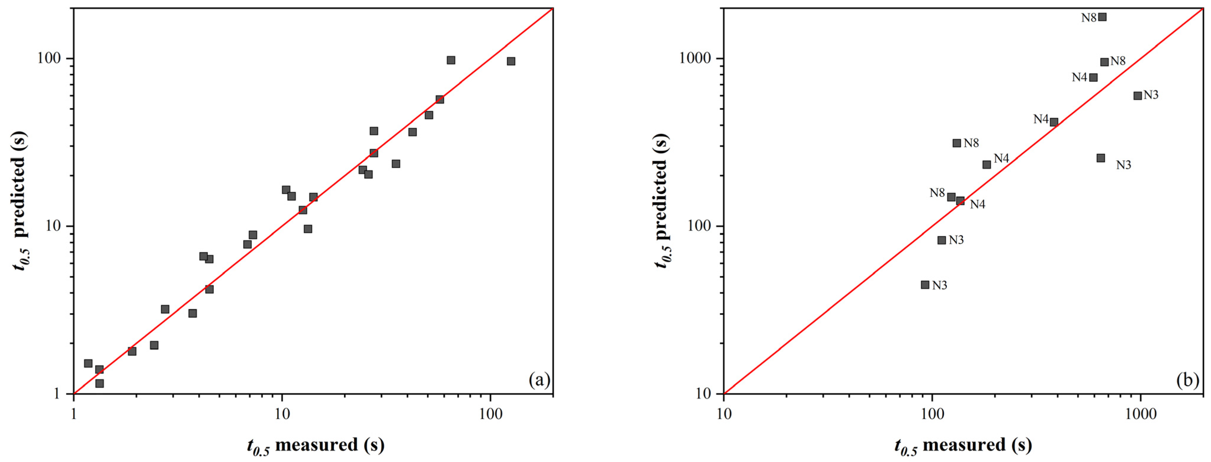
| t0.5 (s) | No SIP | SIP | ||||||||||||||
|---|---|---|---|---|---|---|---|---|---|---|---|---|---|---|---|---|
| Steel | D (µm) | e (-) | 1200 | 1150 | 1100 | 1050 | 1025 | 1000 | 950 | 900 | 850 | 1025 | 1000 | 950 | 900 | 850 |
| N3 | 210 | 0.2 | 1.91 | 7.26 | 24.45 | 57.25 | 111.09 | 970.42 | ||||||||
| 0.35 | 0.77 | 1.33 | 2.44 | 4.49 | 13.34 | 35.29 | 92.56 | 644.69 | ||||||||
| N4 | 190 | 0.2 | 1.33 | 4.47 | 10.46 | 27.66 | 50.76 | 183.03 | 593.68 | |||||||
| 0.35 | 0.72 | 1.33 | 2.75 | 6.84 | 12.60 | 26.01 | 136.56 | 384.77 | ||||||||
| N8 | 140 | 0.2 | 3.73 | 14.17 | 42.33 | 126.00 | 123.68 | 671.66 | ||||||||
| −0.3 | 1.18 | 4.21 | 11.12 | 27.63 | 64.85 | 131.37 | 656.52 | |||||||||
| Steel | Strain (-) | No SIP | SIP | ||
|---|---|---|---|---|---|
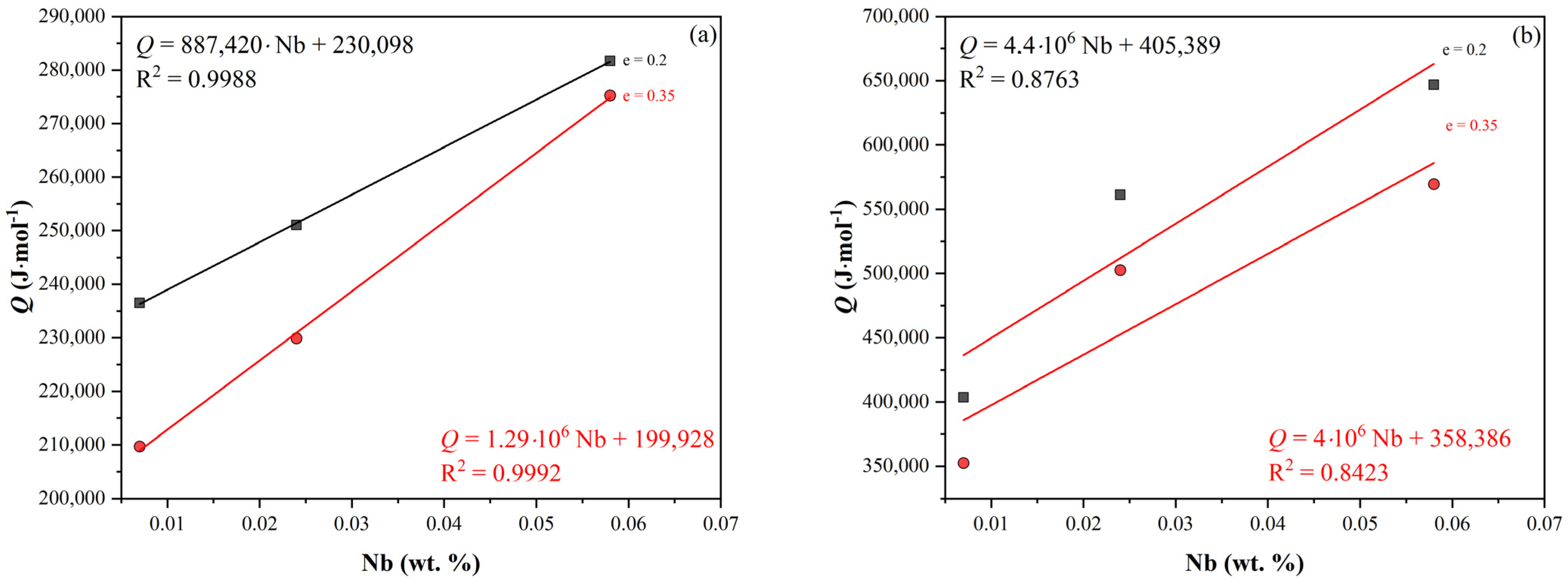
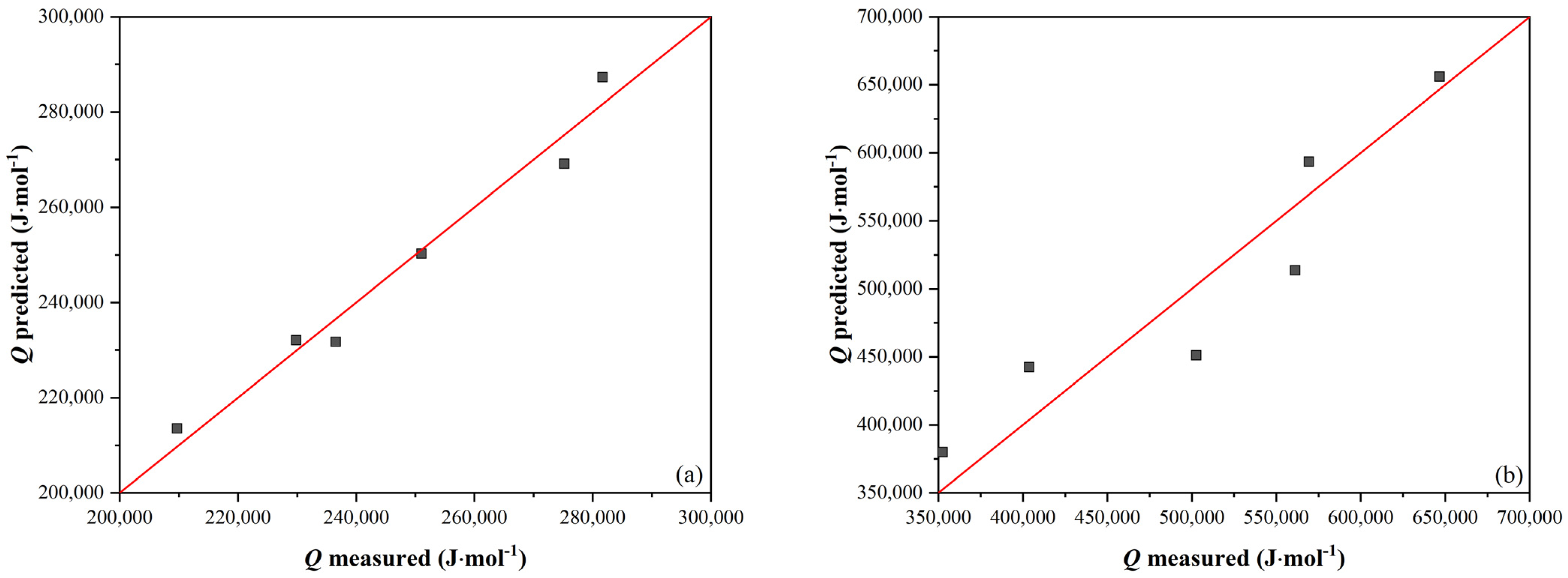
| Q (J·mol−1) | K (-) | Q (J·mol−1) | K (-) | ||
| N3 | 251048 | 1.08 × 10⁻⁹ | 561218 | 1.05 × 10⁻²¹ | |
| N4 | 0.2 | 281684 | 1.11 × 10⁻¹⁰ | 646761 | 1.73 × 10⁻²⁴ |
| N8 | 236541 | 3.37 × 10⁻⁹ | 403719 | 7.09 × 10⁻²⁶ | |
| N3 | 229855 | 4.76 × 10⁻⁹ | 502583 | 2.22 × 10⁻¹⁹ | |
| N4 | 0.35 | 275 192 | 1.09 × 10⁻¹⁰ | 569336 | 1.68 × 10⁻²¹ |
| N8 | 209681 | 1.19 × 10⁻⁸ | 352517 | 2.64 × 10⁻¹⁴ | |
| C | Mn | Si | P | S | Al | Nb | N | Ti |
|---|---|---|---|---|---|---|---|---|
| 0.161 | 1.38 | 0.178 | 0.019 | 0.011 | 0.035 | 0.033 | 0.0044 | 0.001 |
| Variant | D (μm) |
|---|---|
| 1 | 229 |
| 2 | 258 |
| 3 | 240 |
| 4 | 241 |
| Variant | D (μm) | HV 0.3 (-) |
|---|---|---|
| 1 | 96 | 168 |
| 2 | 72 | 183 |
| 3 | 50 | 169 |
| 4 | 46 | 162 |
| No. of Analysis | Ti | Cr | Fe | Nb |
|---|---|---|---|---|
| 1 | 0.9 | 1.6 | 1.8 | 96.6 |
| 2 | 0.6 | 1.6 | 2.4 | 96.0 |
| 3 | 0.8 | 1.4 | 1.9 | 96.4 |
| Mean | 0.77 | 1.53 | 2.03 | 96.33 |
| Std. deviation | 0.153 | 0.115 | 0.321 | 0.306 |
Disclaimer/Publisher’s Note: The statements, opinions and data contained in all publications are solely those of the individual author(s) and contributor(s) and not of MDPI and/or the editor(s). MDPI and/or the editor(s) disclaim responsibility for any injury to people or property resulting from any ideas, methods, instructions or products referred to in the content. |
© 2022 by the authors. Licensee MDPI, Basel, Switzerland. This article is an open access article distributed under the terms and conditions of the Creative Commons Attribution (CC BY) license (https://creativecommons.org/licenses/by/4.0/).
Share and Cite
Sauer, M.; Fabík, R.; Schindler, I.; Kawulok, P.; Opěla, P.; Kawulok, R.; Vodárek, V.; Rusz, S. Analysis of the Microstructure Development of Nb-Microalloyed Steel during Rolling on a Heavy-Section Mill. Materials 2023, 16, 288. https://doi.org/10.3390/ma16010288
Sauer M, Fabík R, Schindler I, Kawulok P, Opěla P, Kawulok R, Vodárek V, Rusz S. Analysis of the Microstructure Development of Nb-Microalloyed Steel during Rolling on a Heavy-Section Mill. Materials. 2023; 16(1):288. https://doi.org/10.3390/ma16010288
Chicago/Turabian StyleSauer, Michal, Richard Fabík, Ivo Schindler, Petr Kawulok, Petr Opěla, Rostislav Kawulok, Vlastimil Vodárek, and Stanislav Rusz. 2023. "Analysis of the Microstructure Development of Nb-Microalloyed Steel during Rolling on a Heavy-Section Mill" Materials 16, no. 1: 288. https://doi.org/10.3390/ma16010288
APA StyleSauer, M., Fabík, R., Schindler, I., Kawulok, P., Opěla, P., Kawulok, R., Vodárek, V., & Rusz, S. (2023). Analysis of the Microstructure Development of Nb-Microalloyed Steel during Rolling on a Heavy-Section Mill. Materials, 16(1), 288. https://doi.org/10.3390/ma16010288


