
Application of Machine Learning in Material Synthesis and Property Prediction

Abstract
:1. Introduction
2. Data Pre-Processing
2.1. Data Collection and Cleaning
2.1.1. Data Collection
2.1.2. Data Cleaning
2.2. Feature Engineering
3. Classification of ML and Algorithms
3.1. Shallow Learning
3.1.1. KNN
3.1.2. DT
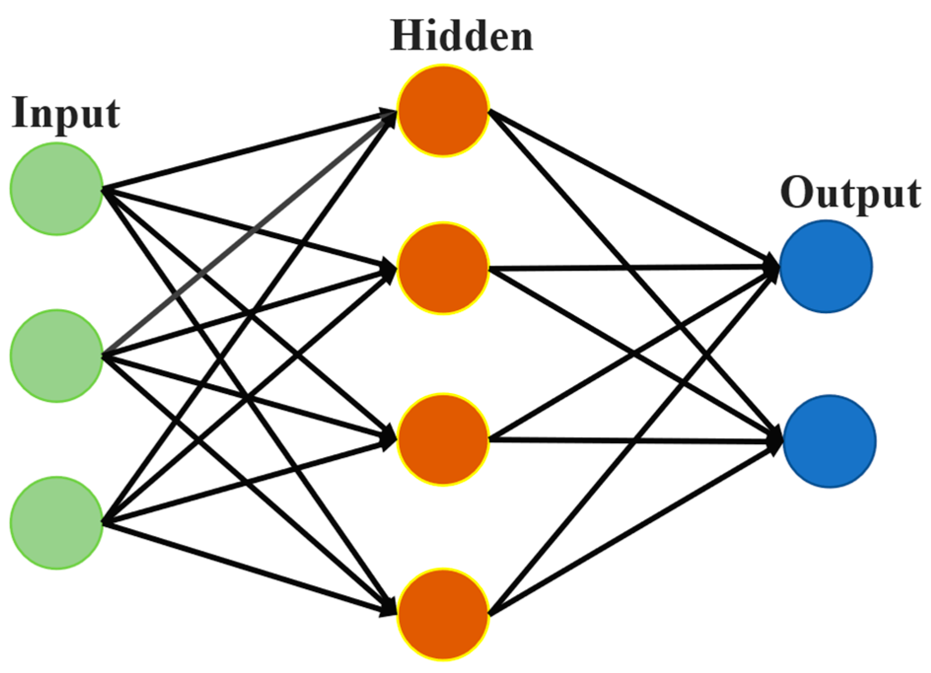
3.1.3. ANN

| Researchers | Algorithms | Purposes |
|---|---|---|
| Sharma et al. [42] | KNN | Predict the fracture toughness of silica-filled epoxy composites. |
| Kumar et al. [43] | KNN | Predict surface roughness in the micro-plasma transfer arc metal additive manufacturing (μ-PTAMAM) process. |
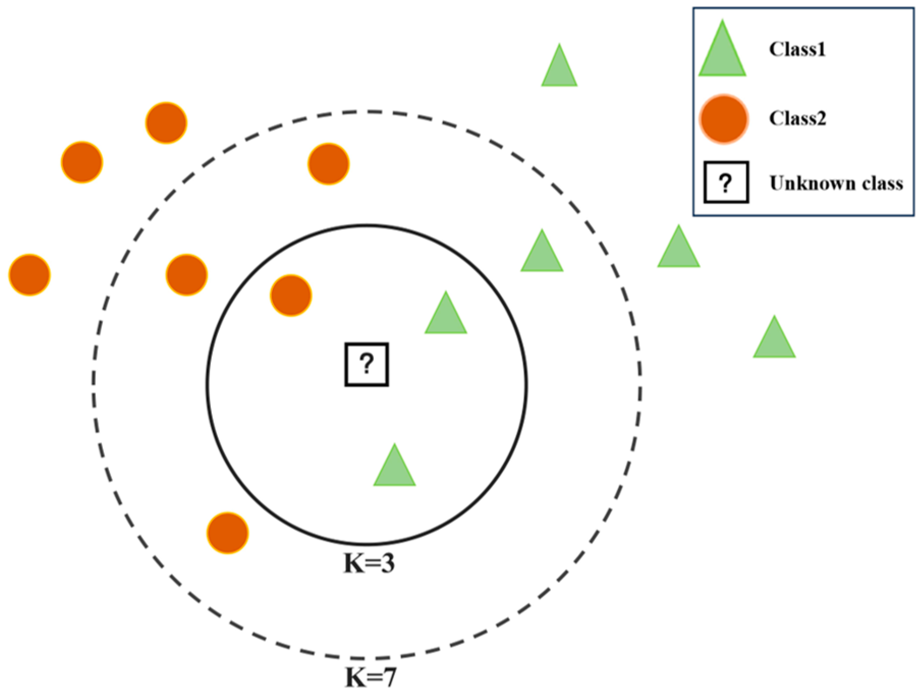
| Jalali et al. [44] | KNN (Figure 6a) | Predict phases in HEAs. |
| Wang et al. [45] | SVM | Achieve rapid detection of transformer winding materials. |
| Martinez et al. [46] | SVM and ANN | Predict the fracture life of martensitic steels under high-temperature creep conditions. |
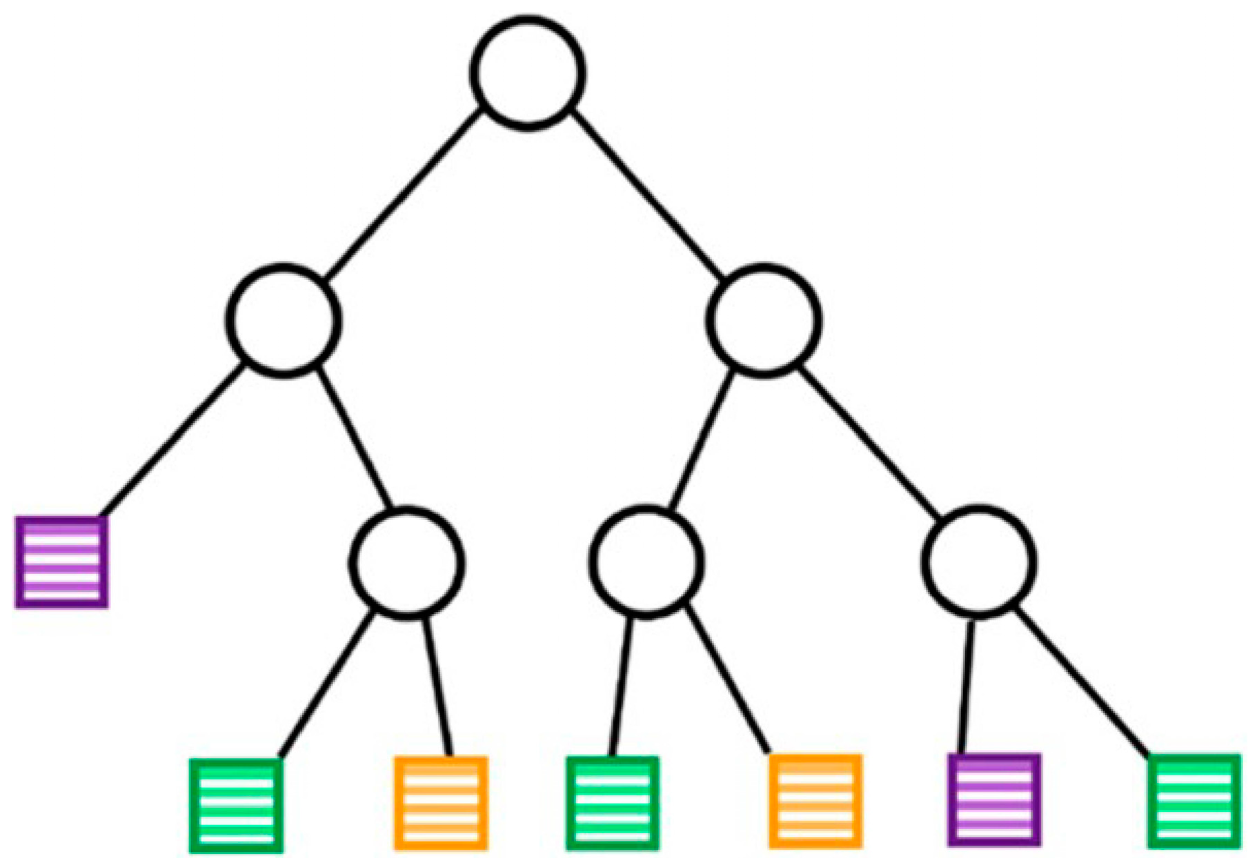
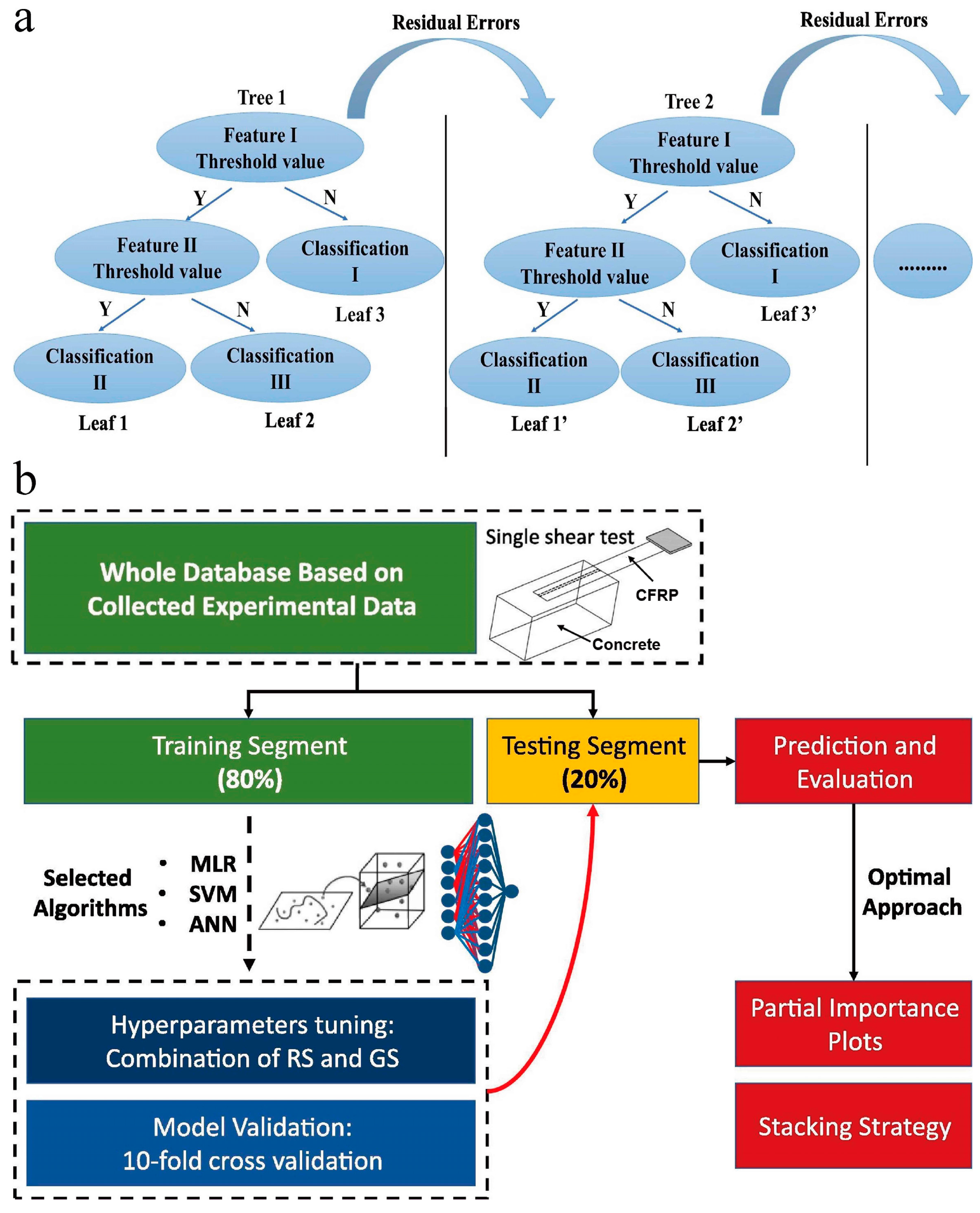
| Ahmad et al. [47] | Adaptive boosting, RF, and DT (Figure 6b) | Predict the compressive strength of concrete at high temperatures. |
| Sun et al. [48] | Gradient boosted regression tree (GBRT) and RF | Evaluate the strength of coal–grout materials. |
| Samadia et al. [49] | GBRT | Predict the higher heating value (HHV) of biomass materials based on proximate analysis. |
| Shahmansouri et al. [50] | ANN (Figure 6c) | Predict the compressive strength of eco-friendly geopolymer concrete incorporating silica fume and natural zeolite. |
| Liu et al. [51] | ANN | Development of a predictive model for the chloride diffusion coefficient in concrete. |

3.2. Deep Learning
3.2.1. Overview of Deep Learning
3.2.2. Applications of Deep Learning
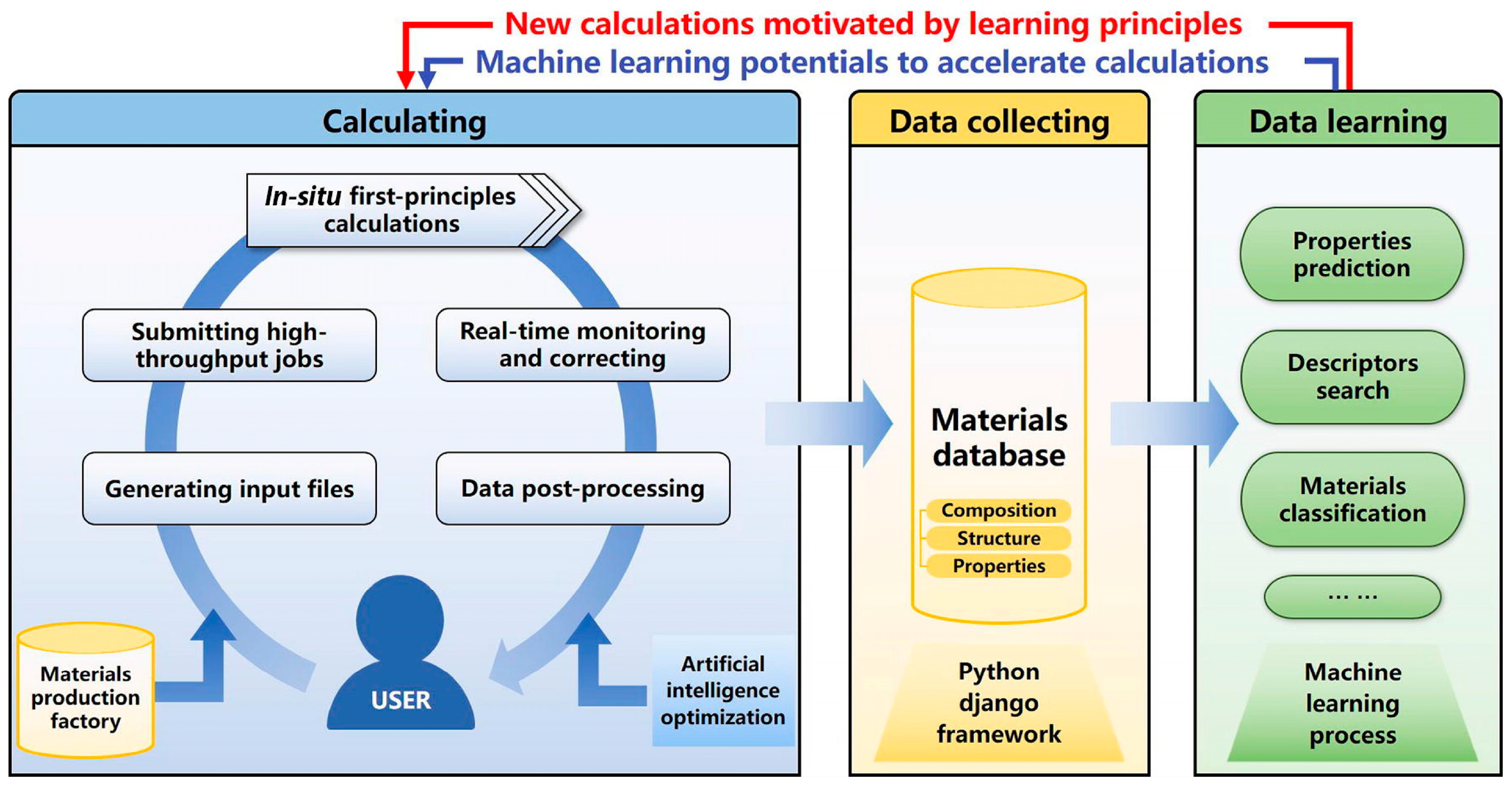
3.3. Materials Informatics Based on ML
4. ML in Materials Science
4.1. Prediction of Material Properties
4.1.1. Molecular Properties
4.1.2. Band Gap
4.1.3. Energy Storage Performance
4.1.4. Structural Health
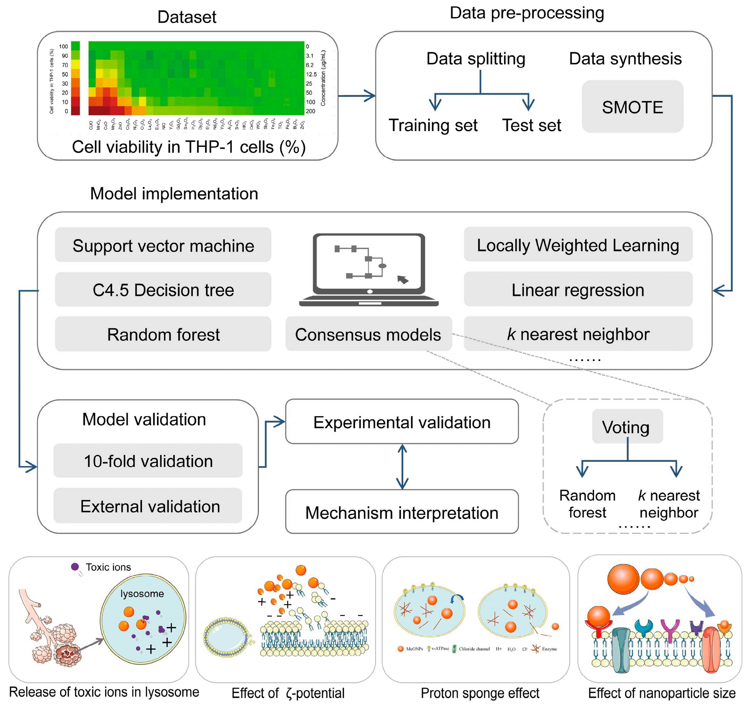
4.1.5. Nanomaterial Toxicity
4.1.6. Adsorption Performance of Nanomaterials
4.2. Accelerated Materials Synthesis and Design
4.2.1. Chalcogenide Materials
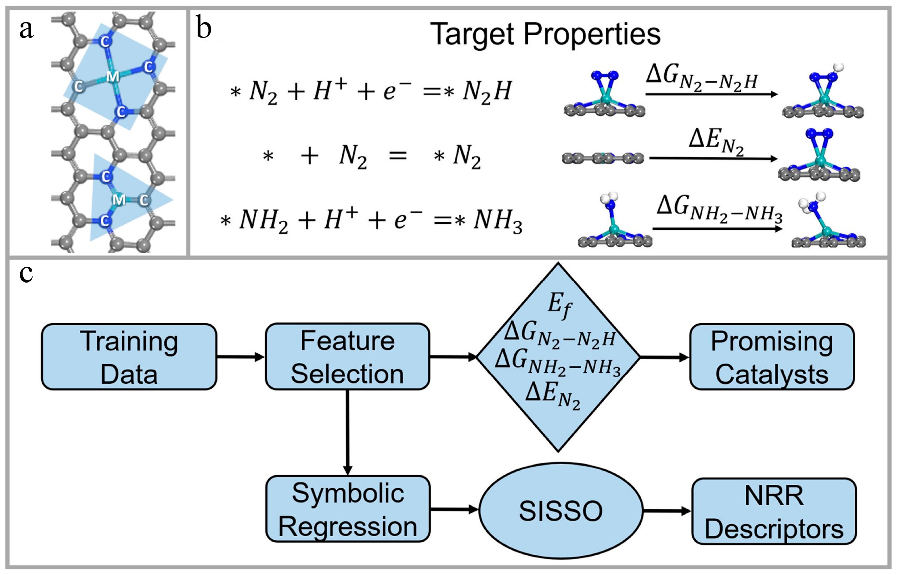
4.2.2. Catalytic Materials
4.2.3. Superconducting Materials
4.2.4. Nanomaterial Outcome Prediction
4.2.5. Nanomaterial Synthesis
4.2.6. Inverse Design of Nanomaterials
5. Conclusions, Challenges, and Prospects
Author Contributions
Funding
Conflicts of Interest
Abbreviations
| ABC | Artificial bee colony |
| AFLOW | Automatic Flow |
| AgNP | Silver nanoparticle |
| AI | Artificial intelligence |
| ANN | Artificial neural network |
| CNN | Convolutional neural network |
| COD | Crystallography Open Database |
| CSD | Cambridge Structural Database |
| DBM | Deep Boltzmann machine |
| DBN | Deep belief network |
| DFT | Density functional theory |
| DNN | Deep neural network |
| DT | Decision tree |
| FDTD | Finite-difference time-domain |
| FRP | Fiber-reinforced polymer |
| GAN | Generative adversarial network |
| GBRT | Gradient boosted regression tree |
| GGA | Generalized gradient approximation |
| GLOnet | Global optimization network |
| HEA | High-entropy alloy |
| HHV | Higher heating value |
| ICA | Imperialist competitive algorithm |
| ICSD | Inorganic Crystal Structure Database |
| JAMIP | Jilin Artificial-intelligence aided Materials-design Integrated Package |
| KNN | K-nearest neighbor |
| LSTM | Long short-term memory |
| MDN | Mixture density network |
| ML | Machine learning |
| MLP | Multilayer perceptron |
| MOF | Metal–organic framework |
| MONC | Metal–organic nanocapsule |
| NMR | Nuclear magnetic resonance |
| OMDB | Organic Materials Database |
| OQMD | Open Quantum Materials Database |
| QD | Quantum dot |
| QSAR | Quantitative structure–activity relationship |
| R-CNN | Region-based CNN |
| ResNet | Residual network |
| RF | Random forest |
| RMSE | Root mean square error |
| RNN | Recurrent neural network |
| SEM | Scanning electron microscope |
| SHM | Structural health monitoring |
| SMILE | Simplified molecular input line entry |
| SVM | Support vector machine |
| SVR | Support vector regression |
| TEM | Transmission electron microscope |
| TGNN | Tupleswise graph neural network |
| UHPC | Ultra-high-performance concrete |
| XGBoost | eXtreme gradient boosting |
| XPS | X-ray photoelectron spectroscopy |
| XRD | X-ray diffraction |
| μ-PTAMAM | Micro-plasma transfer arc metal additive manufacturing |
References
- Lu, S.; Zhou, Q.; Ouyang, Y.; Guo, Y.; Li, Q.; Wang, J. Accelerated discovery of stable lead-free hybrid organic-inorganic perovskites via machine learning. Nat. Commun. 2018, 9, 3405. [Google Scholar] [CrossRef] [PubMed]
- Kolahalam, L.A.; Viswanath, I.K.; Diwakar, B.S.; Govindh, B.; Reddy, V.; Murthy, Y. Review on nanomaterials: Synthesis and applications. Mater. Today Proc. 2019, 18, 2182–2190. [Google Scholar] [CrossRef]
- Schleder, G.R.; Padilha, A.C.; Acosta, C.M.; Costa, M.; Fazzio, A. From DFT to machine learning: Recent approaches to materials science–a review. J. Phys. Mater. 2019, 2, 032001. [Google Scholar] [CrossRef]
- Butler, K.T.; Davies, D.W.; Cartwright, H.; Isayev, O.; Walsh, A. Machine learning for molecular and materials science. Nature 2018, 559, 547–555. [Google Scholar] [CrossRef]
- Chibani, S.; Coudert, F.-X. Machine learning approaches for the prediction of materials properties. APL Mater. 2020, 8, 080701. [Google Scholar] [CrossRef]
- Rajendra, P.; Girisha, A.; Naidu, T.G. Advancement of machine learning in materials science. Mater. Today Proc. 2022, 62, 5503–5507. [Google Scholar] [CrossRef]
- Ruoff, R.; Tse, D.S.; Malhotra, R.; Lorents, D.C. Solubility of fullerene (C60) in a variety of solvents. J. Phys. Chem. 1993, 97, 3379–3383. [Google Scholar] [CrossRef]
- Guo, K.; Yang, Z.; Yu, C.-H.; Buehler, M.J. Artificial intelligence and machine learning in design of mechanical materials. Mater. Horiz. 2021, 8, 1153–1172. [Google Scholar] [CrossRef]
- Cai, J.; Chu, X.; Xu, K.; Li, H.; Wei, J. Machine learning-driven new material discovery. Nanoscale Adv. 2020, 2, 3115–3130. [Google Scholar] [CrossRef]
- Fang, J.; Xie, M.; He, X.; Zhang, J.; Hu, J.; Chen, Y.; Yang, Y.; Jin, Q. Machine learning accelerates the materials discovery. Mater. Today Commun. 2022, 33, 104900. [Google Scholar] [CrossRef]
- Chen, A.; Zhang, X.; Zhou, Z. Machine learning:Accelerating materials development for energy storage and conversion. InfoMat 2020, 2, 553–576. [Google Scholar] [CrossRef]
- Liu, Y.; Niu, C.; Wang, Z.; Gan, Y.; Zhu, Y.; Sun, S.; Shen, T. Machine learning in materials genome initiative: A review. J. Mater. Sci. Technol. 2020, 57, 113–122. [Google Scholar] [CrossRef]
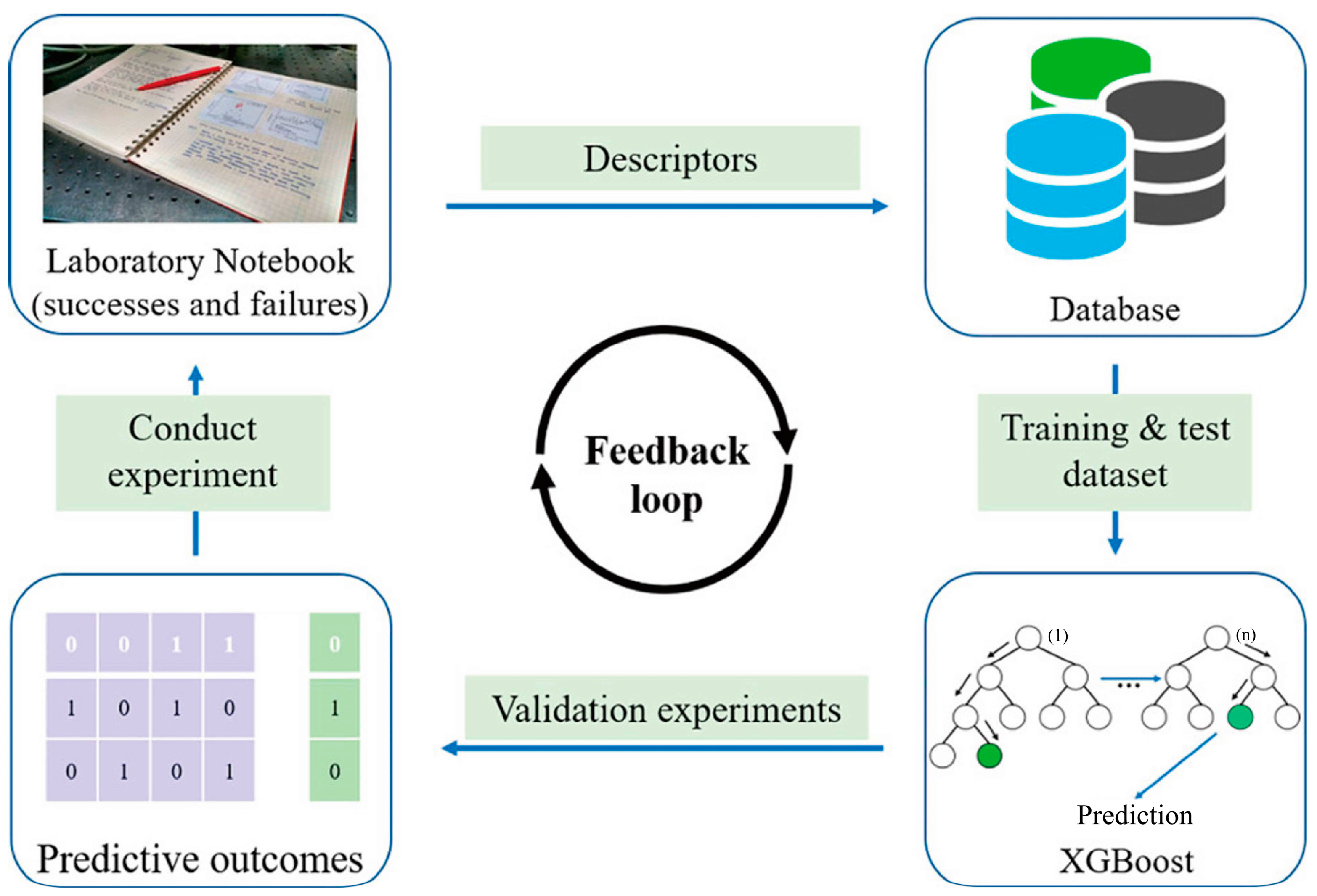
- Raccuglia, P.; Elbert, K.C.; Adler, P.D.; Falk, C.; Wenny, M.B.; Mollo, A.; Zeller, M.; Friedler, S.A.; Schrier, J.; Norquist, A.J. Machine-learning-assisted materials discovery using failed experiments. Nature 2016, 533, 73–76. [Google Scholar] [CrossRef] [PubMed]
- Zhou, L.; Yao, A.M.; Wu, Y.; Hu, Z.; Huang, Y.; Hong, Z. Machine Learning Assisted Prediction of Cathode Materials for Zn-Ion Batteries. Adv. Theory Simul. 2021, 4, 2100196. [Google Scholar] [CrossRef]
- Ridzuan, F.; Zainon, W.M.N.W. A review on data cleansing methods for big data. Procedia Comput. Sci. 2019, 161, 731–738. [Google Scholar] [CrossRef]
- Hossen, M.S. Data preprocess. Machine Learning and Big Data: Concepts, Algorithms, Tools and Applications; Scrivener Publishing: Beverly, MA, USA, 2020; pp. 71–103. [Google Scholar]
- Wu, Y.-W.; Tang, Y.-H.; Tringe, S.G.; Simmons, B.A.; Singer, S.W. MaxBin: An automated binning method to recover individual genomes from metagenomes using an expectation-maximization algorithm. Microbiome 2014, 2, 26. [Google Scholar] [CrossRef]
- Fernández-Delgado, M.; Sirsat, M.S.; Cernadas, E.; Alawadi, S.; Barro, S.; Febrero-Bande, M. An extensive experimental survey of regression methods. Neural Netw. 2019, 111, 11–34. [Google Scholar] [CrossRef]
- Liu, G.-H.; Shen, H.-B.; Yu, D.-J. Prediction of protein–protein interaction sites with machine-learning-based data-cleaning and post-filtering procedures. J. Membr. Biol. 2016, 249, 141–153. [Google Scholar] [CrossRef]
- Wei, J.; Chu, X.; Sun, X.Y.; Xu, K.; Deng, H.X.; Chen, J.; Wei, Z.; Lei, M. Machine learning in materials science. InfoMat 2019, 1, 338–358. [Google Scholar] [CrossRef]
- Wang, M.; Wang, T.; Cai, P.; Chen, X. Nanomaterials Discovery and Design through Machine Learning. Small Methods 2019, 3, 1900025. [Google Scholar] [CrossRef]
- Schmidt, J.; Marques, M.R.G.; Botti, S.; Marques, M.A.L. Recent advances and applications of machine learning in solid-state materials science. NPJ Comput. Mater. 2019, 36, 83. [Google Scholar] [CrossRef]
- Hou, Y.; Wang, Q.; Tan, T. Prediction of carbon dioxide emissions in China using shallow learning with cross validation. Energies 2022, 15, 8642. [Google Scholar] [CrossRef]
- Kurani, A.; Doshi, P.; Vakharia, A.; Shah, M. A comprehensive comparative study of artificial neural network (ANN) and support vector machines (SVM) on stock forecasting. Ann. Data Sci. 2023, 10, 183–208. [Google Scholar] [CrossRef]
- Cover, T.M. Rates of convergence for nearest neighbor procedures. In Proceedings of the Hawaii International Conference on Systems Sciences, Honolulu, HI, USA, 29–30 January 1968. [Google Scholar]
- Peterson, L.E. K-nearest neighbor. Scholarpedia 2009, 4, 1883. [Google Scholar] [CrossRef]
- Sharma, A.; Madhushri, P.; Kushvaha, V. Dynamic fracture toughness prediction of fiber/epoxy composites using K-nearest neighbor (KNN) method. In Handbook of Epoxy/Fiber Composites; Springer: Berlin/Heidelberg, Germany, 2022; pp. 1–16. [Google Scholar]
- Sun, B.; Du, J.; Gao, T. Study on the improvement of K-nearest-neighbor algorithm. In Proceedings of the 2009 International Conference on Artificial Intelligence and Computational Intelligence, Shanghai, China, 7–8 November 2009; pp. 390–393. [Google Scholar]
- Hunt, E. Concept Learning: An Information Processing Problem; John Wiley & Sons, Inc.: Hoboken, NJ, USA, 1962. [Google Scholar]
- Mak, B.; Munakata, T. Rule extraction from expert heuristics: A comparative study of rough sets with neural networks and ID3. Eur. J. Oper. Res. 2002, 136, 212–229. [Google Scholar] [CrossRef]
- Ruggieri, S. Efficient C4. 5 [classification algorithm]. IEEE Trans. Knowl. Data Eng. 2002, 14, 438–444. [Google Scholar] [CrossRef]
- Rokach, L.; Maimon, O. Top-down induction of decision trees classifiers-a survey. IEEE Trans. Syst. Man Cybern. Part C (Appl. Rev.) 2005, 35, 476–487. [Google Scholar] [CrossRef]
- Liu, X.; Liu, T.; Feng, P. Long-term performance prediction framework based on XGBoost decision tree for pultruded FRP composites exposed to water, humidity and alkaline solution. Compos. Struct. 2022, 284, 115184. [Google Scholar] [CrossRef]
- Liu, Y.; Wang, Y.; Zhang, J. New machine learning algorithm: Random forest. In Proceedings of the Information Computing and Applications: Third International Conference, ICICA 2012, Chengde, China, 14–16 September 2012; pp. 246–252. [Google Scholar]
- McCulloch, W.S.; Pitts, W. A logical calculus of the ideas immanent in nervous activity. Bull. Math. Biophys. 1943, 5, 115–133. [Google Scholar] [CrossRef]
- Wu, Y.-C.; Feng, J.-W. Development and application of artificial neural network. Wirel. Pers. Commun. 2018, 102, 1645–1656. [Google Scholar] [CrossRef]
- Huang, Y. Advances in artificial neural networks–methodological development and application. Algorithms 2009, 2, 973–1007. [Google Scholar] [CrossRef]
- Abiodun, O.I.; Jantan, A.; Omolara, A.E.; Dada, K.V.; Mohamed, N.A.; Arshad, H. State-of-the-art in artificial neural network applications: A survey. Heliyon 2018, 4, e00938. [Google Scholar] [CrossRef]
- Hmede, R.; Chapelle, F.; Lapusta, Y. Review of neural network modeling of shape memory alloys. Sensors 2022, 22, 5610. [Google Scholar] [CrossRef]
- Mendizabal, A.; Márquez-Neila, P.; Cotin, S. Simulation of hyperelastic materials in real-time using deep learning. Med. Image Anal. 2020, 59, 101569. [Google Scholar] [CrossRef] [PubMed]
- Savaedi, Z.; Motallebi, R.; Mirzadeh, H. A review of hot deformation behavior and constitutive models to predict flow stress of high-entropy alloys. J. Alloys Compd. 2022, 903, 163964. [Google Scholar] [CrossRef]
- Sharma, A.; Madhushri, P.; Kushvaha, V.; Kumar, A. Prediction of the fracture toughness of silicafilled epoxy composites using K-nearest neighbor (KNN) method. In Proceedings of the 2020 International Conference on Computational Performance Evaluation (ComPE), Shillong, India, 2–4 July 2020; pp. 194–198. [Google Scholar]
- Kumar, P.; Jain, N.K. Surface roughness prediction in micro-plasma transferred arc metal additive manufacturing process using K-nearest neighbors algorithm. Int. J. Adv. Manuf. Technol. 2022, 119, 2985–2997. [Google Scholar] [CrossRef]
- Ghouchan Nezhad Noor Nia, R.; Jalali, M.; Houshmand, M. A Graph-Based k-Nearest Neighbor (KNN) Approach for Predicting Phases in High-Entropy Alloys. Appl. Sci. 2022, 12, 8021. [Google Scholar] [CrossRef]
- Wang, R.; Zheng, Z.; Yin, Z.; Wang, Y. Identification Method of Transformer Winding Material Based on Support Vector Machine. In Proceedings of the 2022 2nd International Conference on Electrical Engineering and Control Science (IC2ECS), Nanjing, China, 16–18 December 2022; pp. 913–917. [Google Scholar]
- Martinez, R.F.; Jimbert, P.; Callejo, L.M.; Barbero, J.I. Material Fracture Life Prediction Under High Temperature Creep Conditions Using Support Vector Machines And Artificial Neural Networks Techniques. In Proceedings of the 2021 31st International Conference on Computer Theory and Applications (ICCTA), Alexandria, Egypt, 11–13 December 2021; pp. 127–132. [Google Scholar]
- Ahmad, M.; Hu, J.-L.; Ahmad, F.; Tang, X.-W.; Amjad, M.; Iqbal, M.J.; Asim, M.; Farooq, A. Supervised learning methods for modeling concrete compressive strength prediction at high temperature. Materials 2021, 14, 1983. [Google Scholar] [CrossRef]
- Sun, Y.; Li, G.; Zhang, N.; Chang, Q.; Xu, J.; Zhang, J. Development of ensemble learning models to evaluate the strength of coal-grout materials. Int. J. Min. Sci. Technol. 2021, 31, 153–162. [Google Scholar] [CrossRef]
- Samadi, S.H.; Ghobadian, B.; Nosrati, M. Prediction of higher heating value of biomass materials based on proximate analysis using gradient boosted regression trees method. Energy Sources Part A Recovery Util. Environ. Eff. 2021, 43, 672–681. [Google Scholar] [CrossRef]
- Shahmansouri, A.A.; Yazdani, M.; Ghanbari, S.; Bengar, H.A.; Jafari, A.; Ghatte, H.F. Artificial neural network model to predict the compressive strength of eco-friendly geopolymer concrete incorporating silica fume and natural zeolite. J. Clean. Prod. 2021, 279, 123697. [Google Scholar] [CrossRef]
- Liu, Q.-F.; Iqbal, M.F.; Yang, J.; Lu, X.-Y.; Zhang, P.; Rauf, M. Prediction of chloride diffusivity in concrete using artificial neural network: Modelling and performance evaluation. Constr. Build. Mater. 2021, 268, 121082. [Google Scholar] [CrossRef]
- Hinton, G.E.; Salakhutdinov, R.R. Reducing the dimensionality of data with neural networks. Science 2006, 313, 504–507. [Google Scholar] [CrossRef] [PubMed]
- Du, X.; Cai, Y.; Wang, S.; Zhang, L. Overview of deep learning. In Proceedings of the 2016 31st Youth Academic Annual Conference of Chinese Association of Automation (YAC), Wuhan, China, 11–13 November 2016; pp. 159–164. [Google Scholar]
- Agrawal, A.; Choudhary, A. Deep materials informatics: Applications of deep learning in materials science. MRS Commun. 2019, 9, 779–792. [Google Scholar] [CrossRef]
- Gu, F.; Khoshelham, K.; Yu, C.; Shang, J. Accurate step length estimation for pedestrian dead reckoning localization using stacked autoencoders. IEEE Trans. Instrum. Meas. 2018, 68, 2705–2713. [Google Scholar] [CrossRef]
- Yang, H.; Shen, S.; Yao, X.; Sheng, M.; Wang, C. Competitive deep-belief networks for underwater acoustic target recognition. Sensors 2018, 18, 952. [Google Scholar] [CrossRef]
- Duong, C.N.; Luu, K.; Quach, K.G.; Bui, T.D. Deep appearance models: A deep boltzmann machine approach for face modeling. Int. J. Comput. Vis. 2019, 127, 437–455. [Google Scholar] [CrossRef]
- Parashar, A.; Raina, P.; Shao, Y.S.; Chen, Y.-H.; Ying, V.A.; Mukkara, A.; Venkatesan, R.; Khailany, B.; Keckler, S.W.; Emer, J. Timeloop: A systematic approach to dnn accelerator evaluation. In Proceedings of the 2019 IEEE International Symposium on Performance Analysis of Systems and Software (ISPASS), Madison, WI, USA, 24–26 March 2019; pp. 304–315. [Google Scholar]
- Gu, J.; Wang, Z.; Kuen, J.; Ma, L.; Shahroudy, A.; Shuai, B.; Liu, T.; Wang, X.; Wang, G.; Cai, J. Recent advances in convolutional neural networks. Pattern Recognit. 2018, 77, 354–377. [Google Scholar] [CrossRef]
- LeCun, Y.; Bengio, Y.; Hinton, G. Deep learning. Nature 2015, 521, 436–444. [Google Scholar] [CrossRef]
- Wu, S.-w.; Yang, J.; Cao, G.-m. Prediction of the Charpy V-notch impact energy of low carbon steel using a shallow neural network and deep learning. Int. J. Miner. Metall. Mater. 2021, 28, 1309–1320. [Google Scholar] [CrossRef]
- Sun, W.; Li, M.; Li, Y.; Wu, Z.; Sun, Y.; Lu, S.; Xiao, Z.; Zhao, B.; Sun, K. The use of deep learning to fast evaluate organic photovoltaic materials. Adv. Theory Simul. 2019, 2, 1800116. [Google Scholar] [CrossRef]
- Konno, T.; Kurokawa, H.; Nabeshima, F.; Sakishita, Y.; Ogawa, R.; Hosako, I.; Maeda, A. Deep learning model for finding new superconductors. Phys. Rev. B 2021, 103, 014509. [Google Scholar] [CrossRef]
- Li, C.; Wang, C.; Sun, M.; Zeng, Y.; Yuan, Y.; Gou, Q.; Wang, G.; Guo, Y.; Pu, X. Correlated RNN Framework to Quickly Generate Molecules with Desired Properties for Energetic Materials in the Low Data Regime. J. Chem. Inf. Model. 2022, 62, 4873–4887. [Google Scholar] [CrossRef] [PubMed]
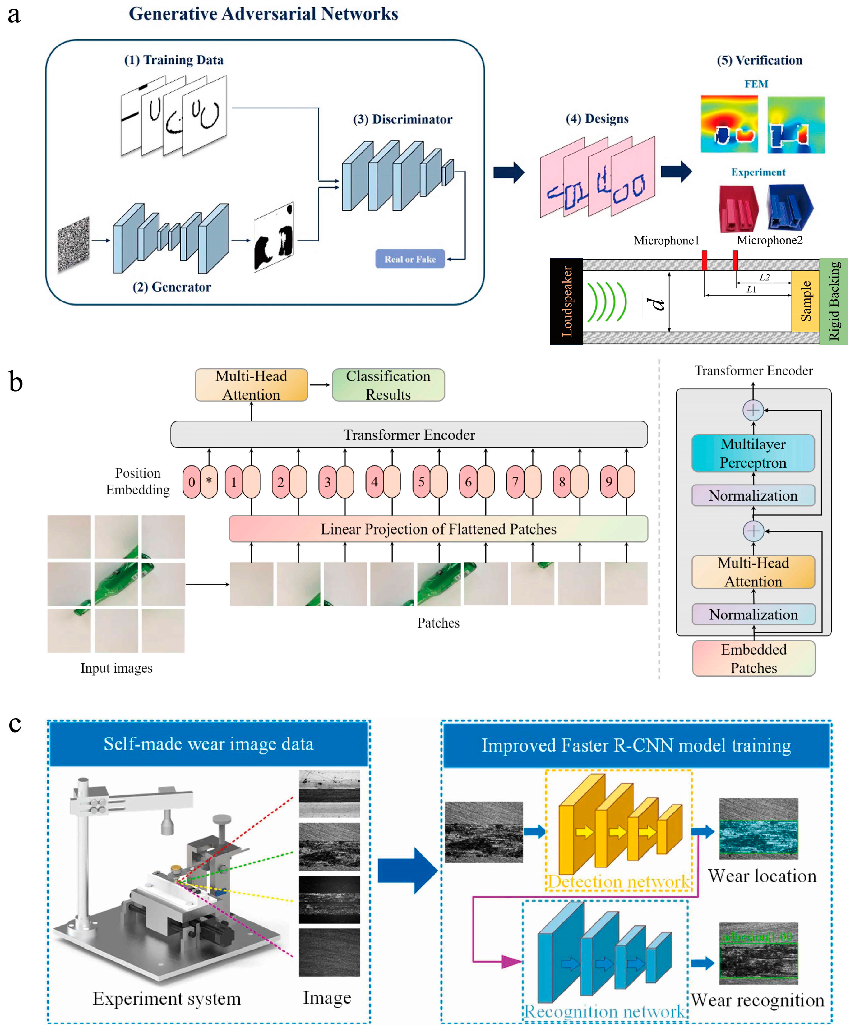
- Zhang, H.; Wang, Y.; Zhao, H.; Lu, K.; Yu, D.; Wen, J. Accelerated topological design of metaporous materials of broadband sound absorption performance by generative adversarial networks. Mater. Des. 2021, 207, 109855. [Google Scholar] [CrossRef]
- Unni, R.; Yao, K.; Zheng, Y. Deep convolutional mixture density network for inverse design of layered photonic structures. ACS Photonics 2020, 7, 2703–2712. [Google Scholar] [CrossRef]
- Huang, K.; Lei, H.; Jiao, Z.; Zhong, Z. Recycling waste classification using vision transformer on portable device. Sustainability 2021, 13, 11572. [Google Scholar] [CrossRef]
- Jiang, J.; Fan, J.A. Multiobjective and categorical global optimization of photonic structures based on ResNet generative neural networks. Nanophotonics 2020, 10, 361–369. [Google Scholar] [CrossRef]
- Wang, M.; Yang, L.; Zhao, Z.; Guo, Y. Intelligent prediction of wear location and mechanism using image identification based on improved Faster R-CNN model. Tribol. Int. 2022, 169, 107466. [Google Scholar] [CrossRef]
- Ramprasad, R.; Batra, R.; Pilania, G.; Mannodi-Kanakkithodi, A.; Kim, C. Machine learning in materials informatics: Recent applications and prospects. NPJ Comput. Mater. 2017, 3, 54. [Google Scholar] [CrossRef]
- Li, M.; Zhang, H.; Li, S.; Zhu, W.; Ke, Y. Machine learning and materials informatics approaches for predicting transverse mechanical properties of unidirectional CFRP composites with microvoids. Mater. Des. 2022, 224, 111340. [Google Scholar] [CrossRef]
- Ramakrishna, S.; Zhang, T.-Y.; Lu, W.-C.; Qian, Q.; Low, J.S.C.; Yune, J.H.R.; Tan, D.Z.L.; Bressan, S.; Sanvito, S.; Kalidindi, S.R. Materials informatics. J. Intell. Manuf. 2019, 30, 2307–2326. [Google Scholar] [CrossRef]
- Al-Saban, O.; Abdellatif, S.O. Optoelectronic materials informatics: Utilizing random-forest machine learning in optimizing the harvesting capabilities of mesostructured-based solar cells. In Proceedings of the 2021 International Telecommunications Conference (ITC-Egypt), Alexandria, Egypt, 13–15 July 2021; pp. 1–4. [Google Scholar]
- Zhao, X.-G.; Zhou, K.; Xing, B.; Zhao, R.; Luo, S.; Li, T.; Sun, Y.; Na, G.; Xie, J.; Yang, X. JAMIP: An artificial-intelligence aided data-driven infrastructure for computational materials informatics. Sci. Bull. 2021, 66, 1973–1985. [Google Scholar] [CrossRef] [PubMed]
- Hu, J.; Stefanov, S.; Song, Y.; Omee, S.S.; Louis, S.-Y.; Siriwardane, E.M.; Zhao, Y.; Wei, L. MaterialsAtlas. org: A materials informatics web app platform for materials discovery and survey of state-of-the-art. NPJ Comput. Mater. 2022, 8, 65. [Google Scholar] [CrossRef]
- Kurotani, A.; Kakiuchi, T.; Kikuchi, J. Solubility prediction from molecular properties and analytical data using an in-phase deep neural network (Ip-DNN). ACS Omega 2021, 6, 14278–14287. [Google Scholar] [CrossRef]
- Liang, Z.; Li, Z.; Zhou, S.; Sun, Y.; Yuan, J.; Zhang, C. Machine-learning exploration of polymer compatibility. Cell Rep. Phys. Sci. 2022, 3, 100931. [Google Scholar] [CrossRef]
- Zeng, S.; Zhao, Y.; Li, G.; Wang, R.; Wang, X.; Ni, J. Atom table convolutional neural networks for an accurate prediction of compounds properties. NPJ Comput. Mater. 2019, 5, 84. [Google Scholar] [CrossRef]
- Venkatraman, V. The utility of composition-based machine learning models for band gap prediction. Comput. Mater. Sci. 2021, 197, 110637. [Google Scholar] [CrossRef]
- Xu, P.; Lu, T.; Ju, L.; Tian, L.; Li, M.; Lu, W. Machine Learning Aided Design of Polymer with Targeted Band Gap Based on DFT Computation. J. Phys. Chem. B 2021, 125, 601–611. [Google Scholar] [CrossRef]
- Espinosa, R.; Ponce, H.; Ortiz-Medina, J. A 3D orthogonal vision-based band-gap prediction using deep learning: A proof of concept. Comput. Mater. Sci. 2022, 202, 110967. [Google Scholar] [CrossRef]
- Wang, T.; Zhang, K.; Thé, J.; Yu, H. Accurate prediction of band gap of materials using stacking machine learning model. Comput. Mater. Sci. 2022, 201, 110899. [Google Scholar] [CrossRef]
- Na, G.S.; Jang, S.; Lee, Y.-L.; Chang, H. Tuplewise material representation based machine learning for accurate band gap prediction. J. Phys. Chem. A 2020, 124, 10616–10623. [Google Scholar] [CrossRef] [PubMed]
- Shen, Z.H.; Liu, H.X.; Shen, Y.; Hu, J.M.; Chen, L.Q.; Nan, C.W. Machine learning in energy storage materials. Interdiscip. Mater. 2022, 1, 175–195. [Google Scholar] [CrossRef]
- Feng, Y.; Tang, W.; Zhang, Y.; Zhang, T.; Shang, Y.; Chi, Q.; Chen, Q.; Lei, Q. Machine learning and microstructure design of polymer nanocomposites for energy storage application. High Volt. 2022, 7, 242–250. [Google Scholar] [CrossRef]
- Yue, D.; Feng, Y.; Liu, X.X.; Yin, J.H.; Zhang, W.C.; Guo, H.; Su, B.; Lei, Q.Q. Prediction of Energy Storage Performance in Polymer Composites Using High-Throughput Stochastic Breakdown Simulation and Machine Learning. Adv. Sci. 2022, 9, 2105773. [Google Scholar] [CrossRef] [PubMed]
- Ojih, J.; Onyekpe, U.; Rodriguez, A.; Hu, J.; Peng, C.; Hu, M. Machine Learning Accelerated Discovery of Promising Thermal Energy Storage Materials with High Heat Capacity. ACS Appl. Mater. Interfaces 2022, 14, 43277–43289. [Google Scholar] [CrossRef] [PubMed]
- Malekloo, A.; Ozer, E.; AlHamaydeh, M.; Girolami, M. Machine learning and structural health monitoring overview with emerging technology and high-dimensional data source highlights. Struct. Health Monit. 2022, 21, 1906–1955. [Google Scholar] [CrossRef]
- Cao, Y.; Miraba, S.; Rafiei, S.; Ghabussi, A.; Bokaei, F.; Baharom, S.; Haramipour, P.; Assilzadeh, H. Economic application of structural health monitoring and internet of things in efficiency of building information modeling. Smart Struct. Syst. 2020, 26, 559–573. [Google Scholar]
- Dang, H.V.; Tatipamula, M.; Nguyen, H.X. Cloud-based digital twinning for structural health monitoring using deep learning. IEEE Trans. Ind. Inform. 2021, 18, 3820–3830. [Google Scholar] [CrossRef]
- Dong, W.; Huang, Y.; Lehane, B.; Ma, G. XGBoost algorithm-based prediction of concrete electrical resistivity for structural health monitoring. Autom. Constr. 2020, 114, 103155. [Google Scholar] [CrossRef]
- Fu, B.; Chen, S.-Z.; Liu, X.-R.; Feng, D.-C. A probabilistic bond strength model for corroded reinforced concrete based on weighted averaging of non-fine-tuned machine learning models. Constr. Build. Mater. 2022, 318, 125767. [Google Scholar] [CrossRef]
- Gao, J.; Koopialipoor, M.; Armaghani, D.J.; Ghabussi, A.; Baharom, S.; Morasaei, A.; Shariati, A.; Khorami, M.; Zhou, J. Evaluating the bond strength of FRP in concrete samples using machine learning methods. Smart Struct. Syst. Int. J. 2020, 26, 403–418. [Google Scholar]
- Li, Z.; Qi, J.; Hu, Y.; Wang, J. Estimation of bond strength between UHPC and reinforcing bars using machine learning approaches. Eng. Struct. 2022, 262, 114311. [Google Scholar] [CrossRef]
- Su, M.; Zhong, Q.; Peng, H.; Li, S. Selected machine learning approaches for predicting the interfacial bond strength between FRPs and concrete. Constr. Build. Mater. 2021, 270, 121456. [Google Scholar] [CrossRef]
- Khan, B.M.; Cohen, Y. Predictive Nanotoxicology: Nanoinformatics Approach to Toxicity Analysis of Nanomaterials. In Machine Learning in Chemical Safety and Health: Fundamentals with Applications; John Wiley & Sons: Hoboken, NJ, USA, 2022; pp. 199–250. [Google Scholar]
- Huang, Y.; Li, X.; Cao, J.; Wei, X.; Li, Y.; Wang, Z.; Cai, X.; Li, R.; Chen, J. Use of dissociation degree in lysosomes to predict metal oxide nanoparticle toxicity in immune cells: Machine learning boosts nano-safety assessment. Environ. Int. 2022, 164, 107258. [Google Scholar] [CrossRef] [PubMed]
- Gousiadou, C.; Marchese Robinson, R.; Kotzabasaki, M.; Doganis, P.; Wilkins, T.; Jia, X.; Sarimveis, H.; Harper, S. Machine learning predictions of concentration-specific aggregate hazard scores of inorganic nanomaterials in embryonic zebrafish. Nanotoxicology 2021, 15, 446–476. [Google Scholar] [CrossRef] [PubMed]
- Liu, L.; Zhang, Z.; Cao, L.; Xiong, Z.; Tang, Y.; Pan, Y. Cytotoxicity of phytosynthesized silver nanoparticles: A meta-analysis by machine learning algorithms. Sustain. Chem. Pharm. 2021, 21, 100425. [Google Scholar] [CrossRef]
- Sajid, M.; Ihsanullah, I.; Khan, M.T.; Baig, N. Nanomaterials-based adsorbents for remediation of microplastics and nanoplastics in aqueous media: A review. Sep. Purif. Technol. 2022, 305, 122453. [Google Scholar] [CrossRef]
- Moosavi, S.; Manta, O.; El-Badry, Y.A.; Hussein, E.E.; El-Bahy, Z.M.; Mohd Fawzi, N.f.B.; Urbonavičius, J.; Moosavi, S.M.H. A study on machine learning methods’ application for dye adsorption prediction onto agricultural waste activated carbon. Nanomaterials 2021, 11, 2734. [Google Scholar] [CrossRef]
- Guo, W.; Liu, J.; Dong, F.; Chen, R.; Das, J.; Ge, W.; Xu, X.; Hong, H. Deep learning models for predicting gas adsorption capacity of nanomaterials. Nanomaterials 2022, 12, 3376. [Google Scholar] [CrossRef]
- Gómez-Bombarelli, R.; Aguilera-Iparraguirre, J.; Hirzel, T.D.; Duvenaud, D.; Maclaurin, D.; Blood-Forsythe, M.A.; Chae, H.S.; Einzinger, M.; Ha, D.-G.; Wu, T. Design of efficient molecular organic light-emitting diodes by a high-throughput virtual screening and experimental approach. Nat. Mater. 2016, 15, 1120–1127. [Google Scholar] [CrossRef]
- Xue, D.; Yuan, R.; Zhou, Y.; Xue, D.; Lookman, T.; Zhang, G.; Ding, X.; Sun, J. Design of high temperature Ti-Pd-Cr shape memory alloys with small thermal hysteresis. Sci. Rep. 2016, 6, 28244. [Google Scholar] [CrossRef] [PubMed]
- Li, W.; Yang, T.; Liu, C.; Huang, Y.; Chen, C.; Pan, H.; Xie, G.; Tai, H.; Jiang, Y.; Wu, Y. Optimizing piezoelectric nanocomposites by high-throughput phase-field simulation and machine learning. Adv. Sci. 2022, 9, 2105550. [Google Scholar] [CrossRef] [PubMed]
- Zhang, L.; He, M.; Shao, S. Machine learning for halide perovskite materials. Nano Energy 2020, 78, 105380. [Google Scholar] [CrossRef]
- Li, L.; Tao, Q.; Xu, P.; Yang, X.; Lu, W.; Li, M. Studies on the regularity of perovskite formation via machine learning. Comput. Mater. Sci. 2021, 199, 110712. [Google Scholar] [CrossRef]
- Liu, H.; Cheng, J.; Dong, H.; Feng, J.; Pang, B.; Tian, Z.; Ma, S.; Xia, F.; Zhang, C.; Dong, L. Screening stable and metastable ABO3 perovskites using machine learning and the materials project. Comput. Mater. Sci. 2020, 177, 109614. [Google Scholar] [CrossRef]
- Omprakash, P.; Manikandan, B.; Sandeep, A.; Shrivastava, R.; Viswesh, P.; Panemangalore, D.B. Graph representational learning for bandgap prediction in varied perovskite crystals. Comput. Mater. Sci. 2021, 196, 110530. [Google Scholar] [CrossRef]
- Wang, Z.; Cai, J.; Wang, Q.; Wu, S.; Li, J. Unsupervised discovery of thin-film photovoltaic materials from unlabeled data. NPJ Comput. Mater. 2021, 7, 128. [Google Scholar] [CrossRef]
- Huang, K.; Zhan, X.-L.; Chen, F.-Q.; Lü, D.-W. Catalyst design for methane oxidative coupling by using artificial neural network and hybrid genetic algorithm. Chem. Eng. Sci. 2003, 58, 81–87. [Google Scholar] [CrossRef]
- Zhang, S.; Lu, S.; Zhang, P.; Tian, J.; Shi, L.; Ling, C.; Zhou, Q.; Wang, J. Accelerated Discovery of Single-Atom Catalysts for Nitrogen Fixation via Machine Learning. Energy Environ. Mater. 2023, 6, e12304. [Google Scholar] [CrossRef]
- Wei, S.; Baek, S.; Yue, H.; Liu, M.; Yun, S.J.; Park, S.; Lee, Y.H.; Zhao, J.; Li, H.; Reyes, K. Machine-learning assisted exploration: Toward the next-generation catalyst for hydrogen evolution reaction. J. Electrochem. Soc. 2021, 168, 126523. [Google Scholar] [CrossRef]
- Hueffel, J.A.; Sperger, T.; Funes-Ardoiz, I.; Ward, J.S.; Rissanen, K.; Schoenebeck, F. Accelerated dinuclear palladium catalyst identification through unsupervised machine learning. Science 2021, 374, 1134–1140. [Google Scholar] [CrossRef] [PubMed]
- Zhang, J.; Zhu, Z.; Xiang, X.-D.; Zhang, K.; Huang, S.; Zhong, C.; Qiu, H.-J.; Hu, K.; Lin, X. Machine learning prediction of superconducting critical temperature through the structural descriptor. J. Phys. Chem. C 2022, 126, 8922–8927. [Google Scholar] [CrossRef]
- Le, T.D.; Noumeir, R.; Quach, H.L.; Kim, J.H.; Kim, J.H.; Kim, H.M. Critical temperature prediction for a superconductor: A variational bayesian neural network approach. IEEE Trans. Appl. Supercond. 2020, 30, 8600105. [Google Scholar] [CrossRef]
- Zhang, J.; Zhang, K.; Xu, S.; Li, Y.; Zhong, C.; Zhao, M.; Qiu, H.-J.; Qin, M.; Xiang, X.-D.; Hu, K. An integrated machine learning model for accurate and robust prediction of superconducting critical temperature. J. Energy Chem. 2023, 78, 232–239. [Google Scholar] [CrossRef]
- Roter, B.; Dordevic, S. Predicting new superconductors and their critical temperatures using machine learning. Phys. C Supercond. Its Appl. 2020, 575, 1353689. [Google Scholar] [CrossRef]
- Pereti, C.; Bernot, K.; Guizouarn, T.; Laufek, F.; Vymazalová, A.; Bindi, L.; Sessoli, R.; Fanelli, D. From individual elements to macroscopic materials: In search of new superconductors via machine learning. NPJ Comput. Mater. 2023, 9, 71. [Google Scholar] [CrossRef]
- Xie, Y.; Zhang, C.; Hu, X.; Zhang, C.; Kelley, S.P.; Atwood, J.L.; Lin, J. Machine learning assisted synthesis of metal–organic nanocapsules. J. Am. Chem. Soc. 2019, 142, 1475–1481. [Google Scholar] [CrossRef]
- Pellegrino, F.; Isopescu, R.; Pellutiè, L.; Sordello, F.; Rossi, A.M.; Ortel, E.; Martra, G.; Hodoroaba, V.-D.; Maurino, V. Machine learning approach for elucidating and predicting the role of synthesis parameters on the shape and size of TiO2 nanoparticles. Sci. Rep. 2020, 10, 18910. [Google Scholar] [CrossRef]
- Tao, H.; Wu, T.; Aldeghi, M.; Wu, T.C.; Aspuru-Guzik, A.; Kumacheva, E. Nanoparticle synthesis assisted by machine learning. Nat. Rev. Mater. 2021, 6, 701–716. [Google Scholar] [CrossRef]
- Braham, E.J.; Cho, J.; Forlano, K.M.; Watson, D.F.; Arròyave, R.; Banerjee, S. Machine learning-directed navigation of synthetic design space: A statistical learning approach to controlling the synthesis of perovskite halide nanoplatelets in the quantum-confined regime. Chem. Mater. 2019, 31, 3281–3292. [Google Scholar] [CrossRef]
- Epps, R.W.; Bowen, M.S.; Volk, A.A.; Abdel-Latif, K.; Han, S.; Reyes, K.G.; Amassian, A.; Abolhasani, M. Artificial chemist: An autonomous quantum dot synthesis bot. Adv. Mater. 2020, 32, 2001626. [Google Scholar] [CrossRef] [PubMed]
- Wang, J.; Wang, Y.; Chen, Y. Inverse design of materials by machine learning. Materials 2022, 15, 1811. [Google Scholar] [CrossRef] [PubMed]
- Li, S.; Barnard, A.S. Inverse Design of Nanoparticles Using Multi-Target Machine Learning. Adv. Theory Simul. 2022, 5, 2100414. [Google Scholar] [CrossRef]
- Wang, R.; Liu, C.; Wei, Y.; Wu, P.; Su, Y.; Zhang, Z. Inverse design of metal nanoparticles based on deep learning. Results Opt. 2021, 5, 100134. [Google Scholar] [CrossRef]
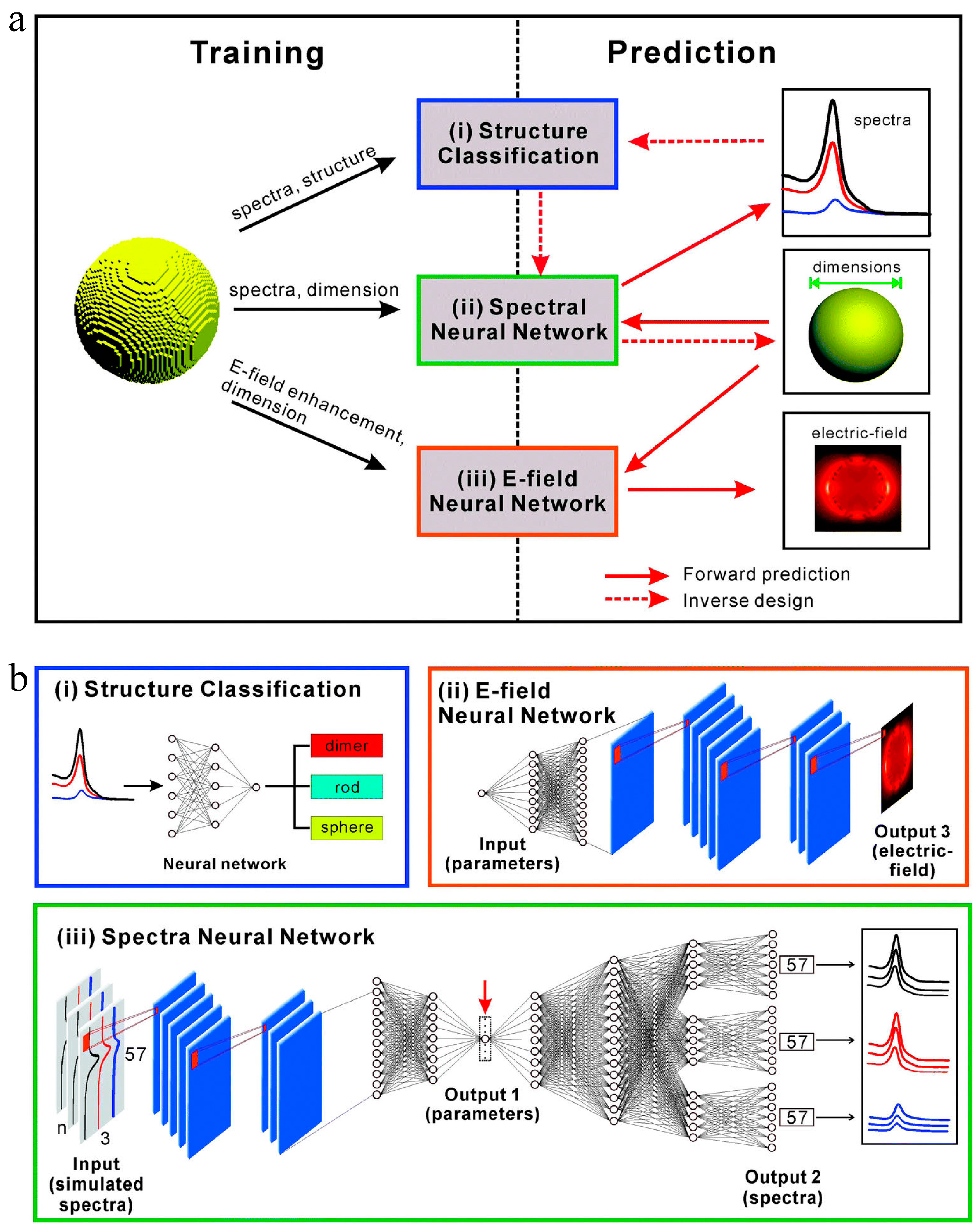
- He, J.; He, C.; Zheng, C.; Wang, Q.; Ye, J. Plasmonic nanoparticle simulations and inverse design using machine learning. Nanoscale 2019, 11, 17444–17459. [Google Scholar] [CrossRef]


| Database | Website | Brief Introduction |
|---|---|---|
| AFLOW | http://www.aflowlib.org/ (accessed on 17 July 2023) | A globally available database of 3,530,330 material compounds with over 734,308,640 calculated properties and growing. |
| Crystallography Open Database (COD) | http://www.crystallography.net/ (accessed on 17 July 2023) | Open-access collection of crystal structures of organic, inorganic, metal–organic compounds and minerals, excluding biopolymers. |
| Cambridge Structural Database (CSD) | https://www.ccdc.cam.ac.uk/ (accessed on 17 July 2023) | The world’s largest database of small-molecule organic and metal–organic crystal structure data, now at over 1.2 million structures. |
| Inorganic Crystal Structure Database (ICSD) | http://cds.dl.ac.uk/ (accessed on 17 July 2023) | A comprehensive collection of crystal structure information for non-organic compounds, including inorganics, ceramics, minerals, and metals, covers the literature from 1915 to the present and contains over 60,000 entries on the crystal structure of in-organic materials. |
| Materials Project | https://materialsproject.org/ (accessed on 17 July 2023) | A database containing 154,718 materials, 4351 intercalation electrodes, and 172,874 molecules. |
| Open Quantum Materials Database (OQMD) | http://oqmd.org/ (accessed on 17 July 2023) | The OQMD is a database of DFT calculated thermodynamic and structural properties of 1,022,603 materials. |
Disclaimer/Publisher’s Note: The statements, opinions and data contained in all publications are solely those of the individual author(s) and contributor(s) and not of MDPI and/or the editor(s). MDPI and/or the editor(s) disclaim responsibility for any injury to people or property resulting from any ideas, methods, instructions or products referred to in the content. |
© 2023 by the authors. Licensee MDPI, Basel, Switzerland. This article is an open access article distributed under the terms and conditions of the Creative Commons Attribution (CC BY) license (https://creativecommons.org/licenses/by/4.0/).
Share and Cite
Huang, G.; Guo, Y.; Chen, Y.; Nie, Z. Application of Machine Learning in Material Synthesis and Property Prediction. Materials 2023, 16, 5977. https://doi.org/10.3390/ma16175977
Huang G, Guo Y, Chen Y, Nie Z. Application of Machine Learning in Material Synthesis and Property Prediction. Materials. 2023; 16(17):5977. https://doi.org/10.3390/ma16175977
Chicago/Turabian StyleHuang, Guannan, Yani Guo, Ye Chen, and Zhengwei Nie. 2023. "Application of Machine Learning in Material Synthesis and Property Prediction" Materials 16, no. 17: 5977. https://doi.org/10.3390/ma16175977
APA StyleHuang, G., Guo, Y., Chen, Y., & Nie, Z. (2023). Application of Machine Learning in Material Synthesis and Property Prediction. Materials, 16(17), 5977. https://doi.org/10.3390/ma16175977