1. Introduction
With the advent of sources, optics and detectors dedicated to X-ray characterization, X-ray diffraction techniques have become highly used tools for the quantitative studies of microstructures in many materials science and engineering applications due to their non-destructive nature and high spatial resolution. Among them, Laue microdiffraction is a spatially resolved X-ray scattering technique which is particularly sensitive to the structural arrangement of atomic lattice planes. It allows the capture of spatial maps of crystallographic orientation and the strain state of (poly)crystalline specimens [
1,
2]. The maps are obtained by systematically scanning the specimens with a polychromatic incident X-ray beam and the subsequent analysis of the resulting scattering patterns recorded on a planar detector. These so-called Laue patterns, as can be seen in
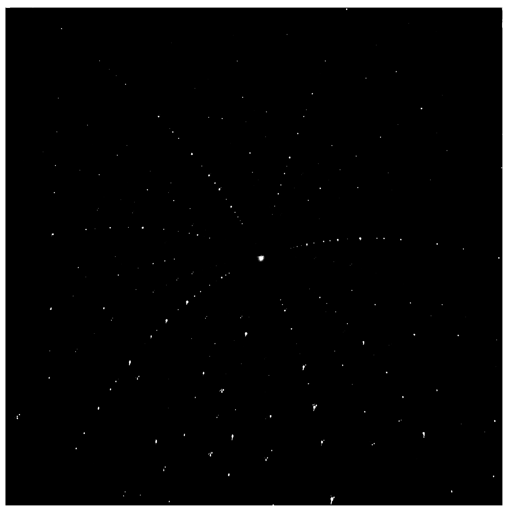
Figure 1, consist of individual Laue spots (i.e., local maxima in the recorded image) which originate from the diffraction phenomena corresponding to geometrical reflections on the lattice planes in the crystals of the probed area in the specimen. Here, each crystal produces a characteristic pattern of spots, all of which superimpose to form the recorded Laue pattern.The precise position of the Laue spots in the experimental Laue pattern is crucial for the reliable determination of the structural crystal parameters, particularly the strain or, equivalently, the lattice parameters of the crystallographic unit cell.
More precisely, the usual workflow for analyzing a Laue pattern of a single probed position in the specimen under consideration consists of three main steps [
3,
4,
5]: first, the local (sub-pixel) maxima in the recorded image are determined, which are assumed to be the positions of the Laue peaks (peak search routine) featuring the geometrical orientation of the corresponding reflecting lattice planes with respect to the incoming X-ray beam direction. Then, for each peak obtained in this way the corresponding crystal and reflecting planes—namely their Miller indices
hkl—are sought (indexing routine). Finally, for each crystal, the lattice parameters of the unit cell of the crystals are refined (given a reference deviatoric strain tensor for the unit cell) by matching the expected/simulated peak positions with the observed ones from the image.
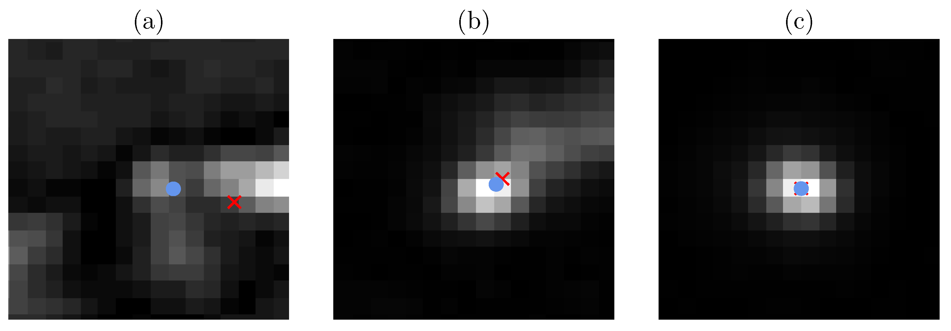
During the peak search step, instead of simply proceeding with the initial peak characterization given by the brightest pixels of a Laue spot, spot shape properties and, most importantly, the peak position have to be estimated with sub-pixel accuracy in order to keep the subsequent analyses as precise as possible. Challenges comprise polycrystalline materials with small variations of orientations and/or strains. Furthermore, the presence of a complicated spatial distribution of extended crystal defects is problematic. The reason for this is that they cause overlapping Laue patterns originating from the individual crystals and complex/non-circular Laue spots, respectively, as can be seen in
Figure 2.
Defining a precise peak position for these multimodal spots that allows for a stable estimation without being affected by small changes in pixel values is hardly possible. The ideal approach would be to split them and treat their subpeaks individually. However, this would involve a complex and time-consuming spot analysis that is unfeasible in practice: currently, several thousands of highly resolved images (
pixel) per dataset corresponding to a raster scan sample map have to be processed. Each of these images in turn contains more than 1000 spots corresponding to the superposition of Laue patterns, each coming from individual grains. In the near future, the demand will increase to several tens of thousands of images with
pixel per image. For this reason, the analysis workflow has to be as fast as possible to keep up with the flood of data measured at synchrotron sources. Recent progress has been made with machine learning approaches to unlock and accelerate the limiting indexing step of Laue patterns [
6,
7], while the previous step of peak search and segmentation has to keep up in order to not be the next performance bottleneck.
Regarding the peak search step, different approaches can be implemented to extract the positions of scattering peaks from digital images. On the one hand, see, e.g., [
8] employed by [
9], relying on image moments [
10] similar to those of bivariate probability distributions. Most importantly, the centroid (which corresponds to the intensity-weighted mean value of the spatial distribution of peak pixels) is used as an estimator for the peak position for further analyses. In order to do this, first, the region of interest (ROI) located at each Laue spot, also known as blob, has to be determined, for which the moments are then computed. The classical strategy to build the ROIs is to apply thresholds [
8], but procedures based on machine learning [
11] have also been proposed. While the image moments are always well defined regardless of whether the spatial distribution of pixel intensities looks like a Laue spot, it is crucial to find well-fitting ROIs that contain exactly one peak in order to obtain valid peak characteristics. Additionally, when a peak is subdivided into several overlapping components, a reliable determination of each individual subpeak is difficult to perform automatically, see, e.g.,
Figure 2a,b.
On the other hand, instead of using the non-parametric approach stated above, other methods are based on fitting a parametric function to the Laue spots, usually using least-squares minimization techniques. For this, mainly Gaussian functions (related to the bivariate normal probability distribution) but also Lorentzian functions (related to the Cauchy probability distribution) or combinations of the two, namely pseudo-Voigt functions, are used [
12,
13,
14]. The parametric approach has the advantage of the descriptors of well-fitting spots being easier to interpret (provided a suitable physical or structural model). Additionally, goodness-of-fit measures can be used as estimates of the model applicability. However, a drawback of the parametric approach is that it can be rather time-consuming when the experimental Laue spot differs from the fitted function.
In the present paper, a procedure using convolutional neural networks (CNNs) is proposed to rapidly estimate the geometric descriptors of Laue spots and select high-quality peaks for a subsequent strain refinement step. While minimum human intervention is sought for the highest throughput in the Laue analysis workflow, relying on a black-box classification system for selecting peaks would make it difficult or even impossible to adapt for difficult specimens/datasets. For this reason, the neural network takes a cutout of the recorded image and returns the precise peak position and key descriptors that are essential for the quality of Laue spots, instead of simply providing a binary decision concerning whether a Laue spot is of good or bad quality. As such, the exact criterion for removing a Laue spot is still explainable and customizable based on these spot descriptors without sacrificing the computational speed.
2. Materials and Methods
In Laue diffraction, a crystal is irradiated with X-rays and the resulting diffraction pattern is captured on a detector. The diffraction pattern consists of a series of peaks, which correspond to the diffraction of the X-rays by the crystal lattice. To analyze the image data collected in this way, the following steps are typically performed (for example, in LaueTools [
14]):
- 1.
Pre-processing: The recorded Laue diffraction image is pre-processed to remove noise and improve the contrast. This may involve techniques such as smoothing, filtering or contrast enhancement.
- 2.
Peak detection: A peak detection algorithm is used to locate the approximate positions of the peaks in the diffraction pattern. This may involve thresholding the image to identify regions of elevated intensity corresponding to the Laue spots, and then using the pixel with the highest intensity as the initial location of the potential peak for each spot.
- 3.
Peak fitting: Once the initial peak positions have been identified, parametric functions (such as a Gaussian or Lorentzian function, which are related to the bivariate normal and Cauchy probability distribution, respectively) are fitted for a precise characterization of the peaks with sub-pixel accuracy.
- 4.
Peak indexing: The positions of the peaks in the diffraction pattern are used to determine the crystal structure. This is performed by comparing the observed peak positions to the expected positions of a known crystal structure, or by using a peak-matching algorithm to determine the most likely crystal structure.
- 5.
Data analysis: The precise characterization of the peaks can be further utilized to determine the crystal structure of each individual crystal, namely the crystallographic unit cell lattice parameters or, equivalently, the strain tensor components. Compiling the results over a dataset of images collected during a sample raster scan allows the imaging of the location of crystals and crystalline defects.
Overall, the process of peak search in Laue diffraction image analysis involves several steps that are designed to identify and analyze the diffraction peaks in the diffraction pattern in order to obtain the structural parameters of experimental crystals. The present paper is concerned with the first step (peak fitting), whose outcome—the accurate characterization of peaks—strongly affects the subsequent steps. The following sections describe the employed methods and materials in detail.
2.1. Description of Experimental Datasets
The Laue diffraction patterns used in the present study were collected during a series of experiments conducted at the BM32 beamline at the European Synchrotron Radiation Facility (ESRF). The data comprise five datasets from a variety of materials, namely defect-free single crystals of Ge, Si, ZnCuOCl and Al2O3, as well as polycrystalline Laue patterns from materials (low-to-high absorption) with strains ranging from 0.001% to 0.2%. This includes a dataset from a thick single crystal of Al2O3, where the elongation of Laue spots is a result of depth effects. These scans were chosen to cover a range of strain levels, as well as to represent different types of crystalline structures.
The Laue diffraction images were collected using top-reflection geometry, where the 2D detector was mounted at the top of the sample and perpendicular to the incoming X-ray beam (collected scattering angles ranging from 2θ = 50°–130° and the sample surface was tilted by 40°. The sample-detector distance for all datasets was between 78.5 mm and 79.5 mm. The X-ray energy used in the experiments was in the range of 5–23 keV with a beam size of approximately 500 × 500 nm.
The images were recorded using a sCMOS detector with a resolution of 2016 × 2018 pixel, a pixel size of 73.4 μm and a bit depth of 16 bits per pixel. Further details regarding the experimental setup at the BM32 beamline—including the synchrotron source, the optics and beamline component—are given in [
15].
2.2. Geometric Characterization of Laue Spots
Before the individual Laue spots can be characterized, they first have to be detected and located in the Laue image. For this reason, an initial approximation of the peak positions is obtained by the peak search algorithm implemented in the LaueTools software package, as can be seen in [
14]. Specifically, connected components in the threshold Laue image, corresponding to the Laue spots, are determined and the initial peak position of each spot is then given by the position of the maximum pixel intensity or the center of mass of these regions. However, not all spots obtained in this way are useful with respect to subsequent Laue image analysis. In particular, it is important to avoid irregular or asymmetrical spots whose description by a simple single crystal model is not relevant. Including such spots in a strain refinement based on a single crystal model provides a poor average estimation of strain levels in the case of crystal defects or the assemblies of crystals. To rapidly detect these hereafter called low-quality Laue spots, a new algorithm was developed to model the shape properties of 2D Laue spots.
For that purpose, a Laue image is written as a map
where
is a rectangular pixel array and
is the 16-bit integer value of the pixel located at
. The array of the pixel intensity values of an individual Laue spot is usually described by a 2D Gaussian function [
16]. More precisely, if we let
be an initial guess of a Laue spot peak position, then normalization constants
should exist such that, for small vectors
, it holds that
. Here,
is a normalized (bivariate) Gaussian function (also known as the probability density of the bivariate normal distribution with vanishing covariances) given by
where
and
are some location and scale parameters, respectively. Thus, to analytically describe the Laue spot at the initially predicted peak position
, the restriction
of the Laue image
to the 32 × 32 pixel cutout
around
is considered, where
denotes the element-wise application of
I on
, in the sense that the output is a matrix
. The normalization constants
as well as the location and scale parameters
and
of the Gaussian function
g are then fitted to the restricted image
using a gradient descent algorithm as implemented in the LaueTools software package [
14].
In the following, we show how 2D Gaussian functions, fitted to image data, can be utilized to effectively characterize Laue spots with respect to their size, shape and position, in order to judge their usefulness for the subsequent strain analysis.
2.2.1. Similarity to a Gaussian Function
As noted in [
5], not all Laue spots are well described by Gaussian functions. Therefore, before analyzing the fitted parameters of a Gaussian function, we first have to verify that it fits well to the image data of the considered Laue spot candidate. For that purpose, we investigate the goodness of fit on the 32 × 32 pixel cutout
introduced above. More specifically, we compute a descriptor of similarity of
and
given by
However, when directly using this similarity descriptor, Laue spot candidates featuring non-Gaussian properties, such as asymmetry (see
Figure 2), will still have a high
-value. On the other hand, Laue spot candidates which appear to be well described by a Gaussian function will usually have a
-value of above 0.95. In order to make the entire interval
descriptive with respect to the goodness of fit, we instead use the rescaled value
to evaluate the similarity of a Laue spot at
to a Gaussian function, where
In cases where the -value is low, the description of Laue spots using the fitted Gaussian functions is not accurate. Thus, such Laue spots should not be used for further analysis.
2.2.2. Precise Peak Position
For the analysis of Laue patterns, the accurate estimation of peak positions is of great importance. For a peak located at the pixel , the peak of the fitted Gaussian function is given by . This precise peak position can achieve sub-pixel accuracy to reliably locate those Laue spots which have a high -value. Similarly to how the fitted location parameters of the Gaussian function are used in order to estimate the sub-pixel peak position of Laue spots, the scale parameters can be used to describe their shape and size.
2.2.3. Shape and Size Descriptors
As mentioned above, it is of great importance to only consider high-quality Laue spots for strain determination in order to achieve the highest reliability. This quality does not only depend on the Gaussian similarity of Laue spots, but also on their shape and size. Hence, in general, large (even symmetrical) elongated spots are discarded. For that reason, we consider the aspect ratio and the size of the spots as featuring descriptors, which are given by
respectively. This multivariate description approach can be utilized to reject or accept spots for strain analysis. However, performing the 2D Gaussian fitting of Laue spots, as stated above, for a large number of Laue images and spots can be rather time-consuming. Thus, we propose an alternative method for the estimation of Laue spot descriptors, which is based on CNNs.
2.3. CNN-Based Prediction of Geometric Spot Descriptors
In order to efficiently determine the peak position
, size
and aspect ratio
of a Laue spot with the preliminary peak position at
, we will directly estimate these descriptors from the image data
corresponding to the Laue spot at
s, instead of using the iterative gradient descent-based approach considered in
Section 2.2.
Since the input
is an image, conventional methods such as linear regression, random forests or dense neural networks [
17] are not suitable. In particular, these approaches do not maintain the spatial correlation of input arguments (i.e., the values
for
), which is of great importance for analyzing image data. For that reason, CNNs, which leverage this spatial structure using convolutions [
18], have been popularized in the literature. In the following, we present details regarding the specific network architecture used in the present paper. For more information on CNNs in general, we refer to [
18,
19].
2.3.1. Adjusted Descriptors
To characterize Laue spots by means of CNNs, some of the descriptors introduced in
Section 2.2, namely the size
and the peak position
, are not suitable. For this reason, these spot descriptors are adjusted. Recall that the (precise) peak position of the Laue spot at
is described by
, while the values of
and
belong to the interval
. Furthermore, note that a spot has low quality if the precise peak position
deviates coordinate-wise by more than 1 from the initially estimated peak position
s, which occurs if
or
. This is due to the fact that the precise peak position
is just a refinement in the sub-pixel scale of the otherwise correct initial peak position
s. Therefore, the values of
and
are only of interest when
. If the precise peak position
deviates coordinate-wise by more than 1 from the initially estimated peak position
s, errors in the prediction of other descriptors could be potentially large, which would overemphasize the effect of those low-quality spots during training. Thus, instead of estimating
for
, we consider the adjusted position
given by
for
Note that the precise peak position
can be reconstructed from
for spots such that
. For the remaining (low-quality) spots, the precise peak position is of no interest as its estimation cannot be assumed to be reliable and these spots will thus be omitted in further analysis.
Similarly, the size descriptor
, given by
, takes values in the set of positive real numbers
. However, since large Laue spots are considered to be of low quality, instead of directly estimating the quantity
, we consider the adjusted size
which takes values in the interval
. Again, for high-quality spots, this adjustment can be reversed. Thus, the quantitative characterization of a Laue spot at
is given by the descriptor vector
. In order to directly estimate this descriptor vector from image data, the CNN architecture stated in the next section is used.
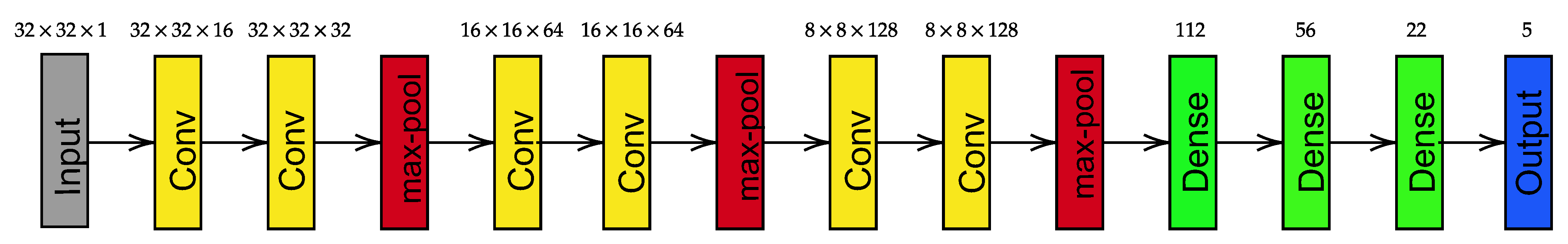
2.3.2. Convolutional Neural Network Architecture
The CNN architecture considered in this paper comprises a fully convolutional stage followed by a fully connected stage, as can be seen in
Figure 3 for a schematic overview. In the fully convolutional stage, convolutional layers with a kernel size of
are iteratively applied with the goal of identifying important features in the images through the convolution with several trainable kernels. Additionally, batch normalization layers are inserted after each convolutional layer. Max-pooling layers with strides of size 2 are applied after the three blocks, consisting of two convolutional layers each. The pooling layers serve the purpose of downsampling the image size, and thus, increasing the effective field of view of the subsequent block of convolutional layers without increasing the number of weights. Since the input image has a resolution of 32 × 32 pixels, (i.e., an array of shape
), the output of the fully convolutional stage is a
-array, which is then used as the input of the fully connected stage.
The following fully connected dense layers have 112, 56, 22 and 5 neurons, respectively, where the last layer represents the final output of the CNN. The activation function of the convolutional layers and the inner dense layers is the ReLU function. The output layer uses a sigmoid function, which can only take values in the interval . In order to use this neural network to the precise estimation of the descriptor vector , the network first has to be calibrated via training, as described below.
2.3.3. Training Procedure
Given the architecture described in
Section 2.3.2, the neural network can be seen as a function
where, for a given input image
, the output also depends on the weights
of the network. To ensure that the network output
approximates the ground truth descriptor vector
reasonably well, we first need to find suitable weights
by training the network. For that purpose, a stochastic gradient descent algorithm with mini-batches of size 32 is used. Specifically, the ADAM optimizer [
19,
20] with a learning rate of 0.001 is applied to minimize the training loss.
The training loss is characterized by means of the
d-dimensional mean absolute error (
), where
corresponds to the five descriptors
,
,
considered in this paper. In the general case of
d descriptors for some
, the loss is given by
where
is an ensemble of
n-true descriptor vectors and
denotes their predictions, with the absolute value norm (also known as
-norm)
for any
.
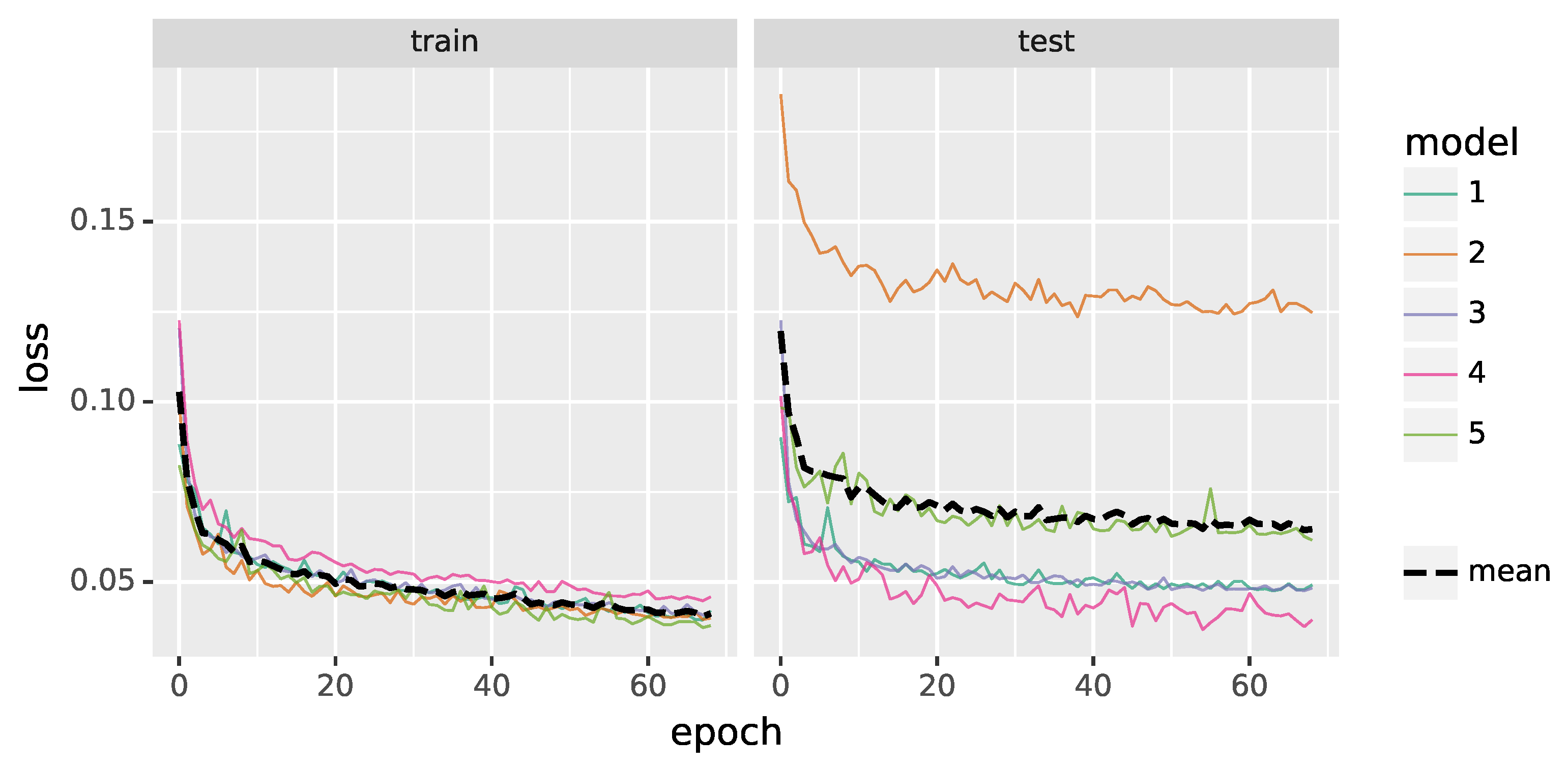
In total, 70 epochs were conducted, with 100 training steps each. To avoid overfitting, the initial model development was performed on a small subset of the first dataset, leading to the choice of various hyperparameters such as the number of epochs and the number of filters in the convolutional stage of the architecture. Additionally, in order to synthetically increase the variance in the training data, input images are shifted, rotated and reflected during training, with the corresponding adjustment of the position descriptor .
2.3.4. Ground Truth Data
As mentioned in
Section 2.1, five Laue microdiffraction scans are available for the training and evaluation of the neural network. From each of these scans, a ground truth dataset
, for
, is obtained by first identifying all Laue spot candidates with the initial peak search algorithm, and then, fitting a 2D Gaussian function to each spot candidate, as can be seen in
Section 2.2. From this, for a spot candidate at
, the true descriptor vector
is determined, which is combined with the image cutout
. Thus, in summary, the ground truth datasets
consist of pairs of input images and corresponding ground truth descriptor vectors for each Laue spot candidate. Since the datasets contain up to 5,000,000 Laue spot candidates, a quasi-random subsampling was conducted to limit the number of Laue spot candidates to 46,000 for each dataset.
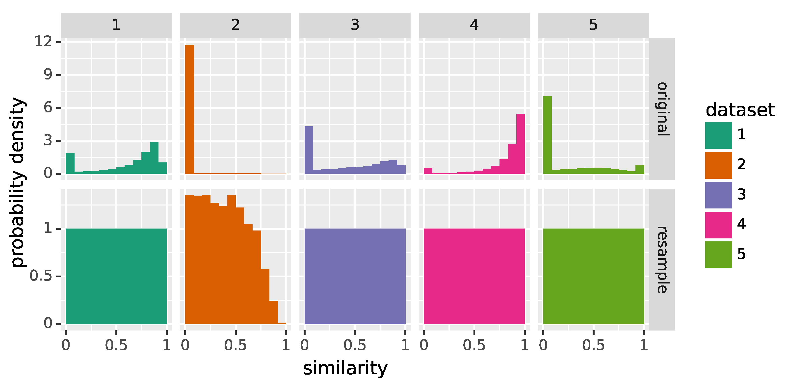
During training, neural networks emphasize the learning of the dependencies between typical values of inputs and outputs. More specifically, these typical values appear more often during training, and thus there is more pressure (i.e., higher training loss) to correctly predict the dependency between them than for other values which occur less often. This can lead to large errors if training and test data follow different probability distributions, as shown in [
21]. Unfortunately, the distribution of the similarity descriptor
varies significantly across the five ground truth datasets, as can be seen in
Figure 4, and this is likely to be true for datasets on which the CNN is applied in the future. To offset these differences, network training is conducted on resampled datasets denoted by
—in fact, as detailed in
Section 3 below, only a selection of these datasets is used during training. The goal of this resampling procedure is to approximate a standard uniform distribution for
, meaning that there are no typical values in the training data. For that purpose, the interval
is partitioned into 12 bins and ground truth pairs (i.e., Laue spots and their descriptor vectors) are assigned to each bin with respect to their similarity descriptor
until they contain 2000 elements. The procedure is also stopped when no pairs remain. For the resulting resampled datasets
, the histograms of the descriptor
are shown in the bottom row of
Figure 4.
4. Discussion
Generally speaking, the following is true for all spot descriptors considered in this paper, with the exception of similarity: to accurately describe a Laue spot as seen in the image data, the underlying Gaussian function has to fit the image data reasonably well. Otherwise, descriptors assume almost arbitrary values. It is thus unsurprising that, by removing bad quality spots from
Table 1, the errors go down as shown in
Table 3.
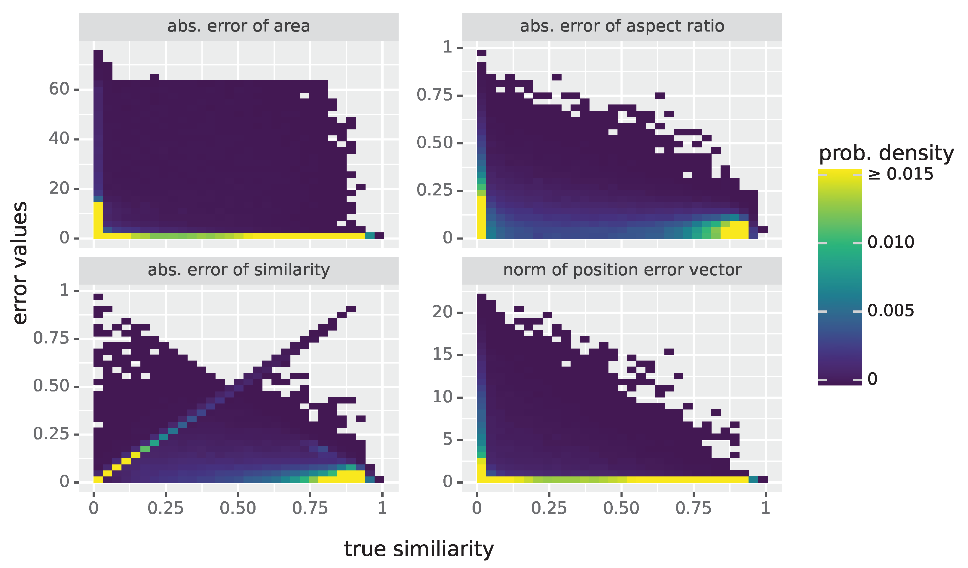
However, the opposite is true for similarity, which is already well predicted on the original data. Here, the coefficient of determination
decreases if only good quality spots are retained. The reason for this is that spots which are obviously badly fitted (i.e., the “easy cases”) are excluded, leaving only the hard cases whose precise value of similarity is more difficult to predict. However, this effect is of little importance for the practical applications of the presented approach, which can be seen by the small numbers of misclassified spots, as can be seen in
Table 2. Only 1.3% of spots are bad-quality spots that are misclassified as good ones. Moreover, the 2.1% of spots which were good-quality spots misclassified as bad ones usually have even less impact in practice, as there are still enough spots for an accurate peak analysis.
Considering only good-quality spots, the peak position is predicted very well, where
and
for aggregated error scores, see
Table 3. The threshold of 0.5 pixels that would nullify the peak position refinement is clearly surpassed even for the worst dataset. In contrast, the aspect ratio is the hardest descriptor to predict for the CNN models with respect to the coefficient of determination. While this descriptor and the area are both simple functions of the scale parameters
and
of the Gaussian function (see
Section 2.2.3), the first one is given as a quotient of
and
in contrast to the second one, which is proportional to their product. The quotient is much more sensitive to slight deviations of
and
, making the estimation less stable compared to the product where errors might cancel out. When considering the mean absolute errors
and
, it is important to keep their respective range in mind: for the first one, values of up to
are possible (as a result of the outlier treatment), whereas for the latter, only values up to 1 occur (as a result of the definition of
).
When analyzing the original distributions of similarity values for each of the five datasets considered in
Figure 4, it becomes clear that they differ substantially from each other, e.g., the second dataset
shows a very skewed distribution where almost all spots are badly fitted by their Gaussian function. This explains the higher error scores shown in
Table 1. As mentioned above this is caused by the ill-defined descriptors for badly fitted spots. When the bad-quality spots are removed from consideration, the resulting score values are more similar to those of the other datasets. Note that in the case of dataset
, only relatively few (175) spots remain, but recall that only a (random) subset of all Laue spots is considered in this evaluation (see
Section 2.3.4).
One idea to improve the prediction performance of the CNNs might be to specifically train models for a single descriptor such as the similarity
. Then, instead of having a single model that predicts all descriptors of interest, multiple models have to be employed. To investigate this further, models were trained with the same cross-validation strategy, as stated in
Section 2.3, but whose output is only
. The error scores listed in
Table 4 show that there is no major improvement compared to the previously considered all-in-one models, despite the significantly increased complexity.
By performing cross-validation on different datasets, the generalization of the prediction performance has been quantified. However, there might be further aspects that impact the performance. While the crystal structure and orientation govern the position of the diffraction peak, the shape of the Laue spot depends on the local crystal misorientation distribution within the probed volume. The datasets considered in the present paper were chosen to comprise a wide variety of spot shapes from simple ones, which are well described by Gaussian functions, to very complex ones. For this reason, we assume that the predictor will work equally well on other datasets whose local crystal misorientation distribution is within the considered spectrum, irrespective of crystal structures. Nevertheless, before applying it to datasets that are outside this broad spectrum, the prediction quality should be reevaluated. Another aspect that concerns the generalization is the distance between the sample and the detector. As mentioned above the datasets considered in the present paper were acquired with a distance between 78.5 mm and 79.5 mm. Increasing this distance leads to a homothetical transform that enlarges the Laue spots, but leaves their general shape intact. The size of the cutouts (32 × 32 pixels) that are fed to the CNN models was chosen to work well for these values of the detector distance. However, for much larger values, the Laue spots might not fully fit into the cutouts and the CNN models would thus be unable to describe them accurately. In this case, the models would need to be retrained with a larger cutout size, (e.g., 64 × 64 pixels instead of 32 × 32 pixels).
One of the main advantages of the CNN-based estimator presented in this paper is its high computational speed. To make this clear, the runtime performance was evaluated by comparing it to that of the conventional gradient descent approach implemented in LaueTools, see [
14]. For this purpose, 10 repetitions of analyzing 10,000 Laue spots were conducted to determine the timings reported in
Table 5.
The evaluation procedure of the runtime performance consists of two setups: As the gradient descent only uses a single processor core, the CNN-based approach was also been restricted to a single core in the first setup for a fair comparison. In this case, an acceleration of 2.089 ms/0.647 ms = 3.23 is obtained, as can be seen in
Table 5. In the second setup, the predictions of the neural network are computed on a GPU. Here, a speedup of 2.089 ms/0.027 ms = 77 is achieved. While the CNN-based approach is already significantly faster for the single-threaded setup, on the GPU, it can fully leverage its inherent affinity for parallel computing, resulting in massive speedups. It is also worth mentioning that the runtime for the CNN stays the same for all inputs, whereas the gradient descent algorithm takes longer for difficult test datasets with many bad-quality spots (such as
). The reason for this is that, for irregular spots, the initial parameters based on pixel values do not already lead to a good fit and several iterations of optimization steps must be computed. The experiments were performed on an AMD Ryzen 9 3900x CPU and an NVIDIA RTX 2080 Super GPU.
5. Conclusions
In this paper, we described a CNN-based method for the characterization of Laue spots (given by a pixel intensity distribution), which is an important step when analyzing Laue patterns. With the presented method, the conventional approach based on the computationally expensive fitting of parametric functions can be replaced by fast CNNs. As such, a significant acceleration (up to 77 times when using a GPU) is achieved for the prediction of geometric spot descriptors.
Using the CNN-based method, descriptors derived from the fitted Gaussian functions can be accurately estimated for Laue spots that are well described by these functions (good-quality spots). The remaining spots have little similarity to the parametric functions, and thus, descriptors derived from these fitted parametric functions assume almost arbitrary values. For this reason, such spots are not useful for the subsequent analysis. The CNN allows to quantify this similarity and, in this way, the usefulness of a Laue spot descriptors for the subsequent analysis.
While the currently predicted spot descriptors could be estimated using traditional (albeit slower) methods, the approach proposed in the present paper can also be applied to other descriptors which are more difficult to estimate by traditional methods. For example, there is the occurrence of so-called “double peaks” which occur when two Laue spots overlap. By synthetically overlapping the grayscale images of multiple Laue spots, we could synthetically generate the realistic training data of double peaks, where descriptors for both peaks are well known. These data could be used to train a neural network in order to learn the descriptors of double peaks, which would allow us to further analyze Laue spots that are currently not well described by parametric functions.


 ,
, 


