Abstract
In order to describe the dependence of critical current on specimen length and crack size distribution in the superconducting tape with cracks of different sizes, a Monte Carlo simulation and a model analysis were carried out, employing the model specimens of various lengths constituted of multiple short sections with a crack per each. The model analysis was carried out to evaluate the effects of the two factors on the critical current of a specimen. Factor 1 is the size of the largest crack in a specimen, and Factor 2 is the difference in crack size among all sections at the critical voltage of critical current. Factors 1 and 2 were monitored by the smallest ligament parameter among all sections constituting the specimen and by the number of sections equivalent to the section containing the largest crack at the critical voltage of the critical current of the specimen, respectively. The research using the monitoring method revealed quantitatively that the critical current-reducing effect with increasing specimen length is caused by the increase in the size of the largest crack (Factor 1), and also, the critical current-raising effect is caused by the increase in the difference of crack size (Factor 2). As the effect of Factor 1 is larger than that of Factor 2, the critical current decreases with increasing specimen length. With the present approach, the critical current reducing and raising effects under various crack size distributions were evaluated quantitatively as a function of specimen length, and the specimen length-dependence of critical current obtained by the Monte Carlo simulation was described well.
1. Introduction
Critical current Ic (estimated by application of the electrical field criterion Ec = 1 µV/cm to the voltage V—current I curve) and n-value (estimated as the index n of the approximated I ∝ In curve in the electrical field range of E = 0.1~10 µV/cm) are reduced under high electromagnetic and mechanic stresses, as have been reported for the superconducting oxide (such as RE(Y, Sm, Dy, Gd,···)Ba2Cu3O7-δ: REBCCO) layer-coated tape [1,2,3,4,5,6,7,8,9,10,11,12,13,14], and Bi2223 [15,16,17,18,19,20]-, MgB2 [21,22,23,24,25]- and Nb3Sn [26,27,28,29,30,31]-filamentary types. In this work, we conduct a fundamental study on the influences of cracks in superconducting layer-coated tape on Ic. Usually, the cracking takes place non-uniformly, and hence, the Ic/n-values vary by specimen [3,7,13,18] and along the length of the specimen [7,13,14]. Not limited to the stress-induced cracks, the non-uniformly distributed defects introduced during the fabrication process also cause a reduction in Ic and n-values [11,13]. For safety design, it is required to reveal the relation of non-uniformly distributed defects/cracks to superconducting property [32].
In studying the effect of crack size distribution and specimen length on Ic and n-values, the authors used a Monte Carlo simulation method [13,14] combined with a current shunting model of cracks [17]. From the simulation results using the model specimens consisting of multiple short sections with cracks of different sizes, the following results have been obtained: (i) The section with the largest crack contributes most significantly to the synthesis of the V–I curve of the specimen. (ii) The Ic-value of a specimen is determined by the size of the largest crack in the specimen as a first approximation when the specimen is short but not when the specimen is long [9]. The size of the largest crack determines the Ic value of the specimen as a first approximation when the specimen is short but not when the specimen is long [13]. This result suggests that the Ic value is determined not only by the effect of the largest crack but also by an effect whose contribution to Ic becomes greater the longer the specimen.
Motivated by the results above, we attempted to describe the specimen length-dependence of the Ic value based on the effects of two factors. Factor 1 is the size of the largest crack in the specimen. Factor 2 is the difference in size among cracks at the critical voltage of the critical current of the specimen. As the research tools, we used the monitoring method for numerical estimation of the effect of Factor 1 and Factor 2, together with the Monte Carlo simulation method [13,14] and Gumbel’s extreme value distribution function [33].
2. Materials and Methods
2.1. Simulation to Obtain Critical Current Values under Various Specimen Lengths and Various Distribution Widths of Crack Size
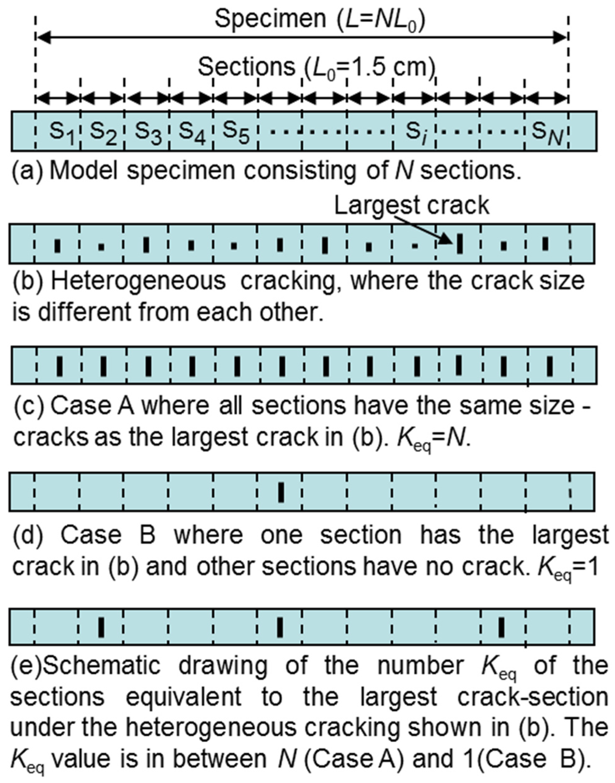
Figure 1 shows (a) a model specimen of a superconducting layer such as REBCCO-layer-coated tape, containing N local sections with a length L0 = 1.5 cm and one crack per each, (b) heterogeneously cracked superconducting layer, (c) extreme Case A, (d) extreme Case B and (e) array of the largest crack in the intermediate case between Cases A and B, which were used as the tools to estimate the effects of Factor 1 and Factor 2 on Ic. as follows:
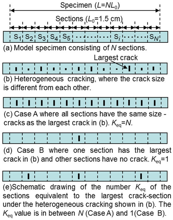
Figure 1.
Schematic drawing of the model specimen and array of cracks for analysis. (a) Model specimen consisting of N local sections that have a length L0 = 1.5 cm and one crack in each. (b) Heterogeneous cracking in the model specimen. (c,d) The extreme Case A and Case B, giving the lower- and upper- bound of critical current, respectively. (e) Drawing of an example of the number of the sections equivalent to the largest crack-section Keq estimated from the heterogeneous cracking shown in (b) by the procedure shown later in Section 2.2. The Keq-value is in between N (Case A) and 1 (Case B). The case of Keq = 3 is drawn as an example. The specimen length (voltage probe distance) L = NL0 length L = 1.5~60 cm under various crack size distributions were obtained by Monte Carlo simulation [13,14] combined with the crack-induced current shunting model [17].
The simulation was carried out in the following procedure. Then, the simulation results were analyzed to clarify the effect of Factor 1 (size of the largest crack) and Factor 2 (difference of crack size at the critical voltage of critical current of the specimen) on the Ic of the specimen by applying the method and procedure in Section 2.2.
The following technical terms were used. “f and 1 − f: ratios of cross-sectional area of the cracked- and ligament-parts to the total cross-sectional area of the superconducting layer, respectively”, “IRE: current transported by the superconducting layer in the ligament part”, “Is: crack-induced shunting current”, “Rt: electrical resistance of the shunting circuit”, “VRE: voltage developed at the ligament part that transports current IRE, being equal to the voltage vs. (=IsRt) developed at the cracked part by shunting current Is, since the cracked part and the ligament part constitute a parallel electrical circuit”, “Ic0 and n0: critical current and n-value of the sections in the non-cracked state, respectively”, “Ec (=1 μV/cm): critical electrical field for determination of the critical current value”, “s (<<L0): current transfer length”, “Lp: ligament parameter of section, given by Lp = (1 − f)(L0/s)1/n0, which was derived by the authors [13,14] through a modification of the formulations of Fang et al. [17]”, and “ΔLp: standard deviation of the ligament parameter Lp”.
The cross-sectional area of ligament 1 − f and crack f have a one-to-one relation; the smaller the ligament, the larger the crack. The ligament parameter Lp, which is proportional to 1 − f, was used as a monitor of 1 − f and f. Accordingly, the size of the largest crack is expressed by the smallest ligament parameter Lp,smallest. The standard deviation of 1 − f and f is the same. Thus, the standard deviation ΔLp of the ligament area fraction 1 − f is the same as that of the crack area fraction f. Hence, the standard deviation of the ligament parameter, ΔLp, was used as a monitor of the distribution width of crack size and ligament size. As well as that of crack size, the larger the ΔLp value, the wider the distribution of both the crack size- and ligament size.
The distribution of Lp was formulated by the normal distribution function as an example. Noting the average of Lp values as Lp,ave, the cumulative probability F(Lp) and density probability f(Lp) are expressed by:
In the Monte Carlo simulation, the Lp value for each section was set by the following process. The Lp,ave was taken to be 0.667, which refers to a situation where the average crack size is ≈1/3. The standard deviation of Lp, ΔLp was set to be 0.01, 0.025, 0.05, 0.10, and 0.15. Using the values mentioned above, the Lp value was given for each cracked section by generating a random value in the range of 0~1, setting F(Lp) = generated random value, and substituting the values of Lp,ave (=0.667) and ΔLp (0.01–0.15) in Equation (1).
For the section without crack, the voltage (I)—current (I) relation is expressed by:
The transport current in a cracked section is the sum (I = Is + IRE) of the shunting current Is in the cracked part and superconducting layer (for instance, REBCO)-transported current IRE in the ligament part. The V–I curve of the cracked section is expressed as:
We calculated the V–I curve of the non-cracked section by substituting L0 = 1.5 cm, Ic0 = 200 A, and n0 = 40 taken from the experimental result of DyBCO coated conductor [3], into Equation (3), and also V–I curve of the cracked section by substituting the Lp value given in the Monte Carlo method and the values mentioned above into Equations (4) and (5).
Since the specimen consists of a series electrical circuit of N sections (Figure 1a,b), the current I in the specimen is the same as that in all sections (Equation (6)), and the voltage of the specimen is the sum of the voltages of all sections (Equation (7)).
I = ISi (i = 1 to N)
The V–I curves of the specimens were synthesized with the V–I curves of the sections using Equations (6) and (7). Using the V–I curves of the sections and specimens, the Ic values of the sections and specimens were obtained using the electrical field criterion of Ec = 1 μV/cm.
2.2. Model Analysis of the Specimen Length (L)-Dependence of Critical Current (Ic) under Various Distribution-Widths of Crack Size (ΔLp)
A series of sections with cracks of different sizes (Figure 1b) constructs a specimen.
With increasing applied current, the superconductivity of the specimen is lost first in the section with the largest crack since the voltage developed at the largest crack section is highest among all sections, and hence, it contributes most to the voltage of the specimen. The ligament parameter of the largest crack section is the smallest among all sections. It is noted as Lp,smallest. Factor 1 (largest crack in the specimen) was monitored by Lp,smallest. When the Lp,smallest value is known, the lower and upper bounds of critical current can be calculated using the extreme Case A and Case B [13,14], as follows.
Case A is an extreme case where the crack size is the same as the largest of all sections, as shown in Figure 1c, and the V–I curves of all sections are the same. Accordingly, the voltage of the specimen, given by the sum of the crack size of the voltages of all sections, corresponds to the upper bound of the voltage of the specimen, Vupper. As Vupper reaches Vc at the lowest current, the Ic value in Case A is the lower bound, Ic,lower.
Case B is another extreme case where the crack size of one section is far larger than that of the other sections, as shown in Figure 1d, and the voltages developed at the cracks in the other sections are too low to contribute to the voltage of the specimen. This case gives the lower bound of the voltage of specimen Vlower. As Vlower reaches Vc at the highest current, the Ic value in Case B is the higher bound, Ic,upper, under the given largest crack size, monitored by Lp,smallest.
In this way, the Vupper–I curve and Ic,lower are given by Case A, and the Vlower–I curve and Ic,upper are given by Case B due to the difference in the number of the largest cracks; N in Case A and 1 in Case B.
As shown in Figure 1b, cracks of various sizes exist in practical specimens. Accordingly, the largest crack section and the other sections contribute to the voltage of the specimen. The extent of the contribution of the other sections is seen in the positional relation among the V–I curves of the sections, reflecting the distribution-width of crack size ΔLp; when ΔLp is small, the V–I curves of sections exist near each other and hence the voltage of the specimen (=sum of the voltages of sections) tends to be high, while, when ΔLp is large, the V–I curves of sections exist apart to each other and hence voltage of the specimen tends to be low. This means that the difference in the size of cracks is an important factor in determining the Ic value.
The effect of the difference in size among cracks (Factor 2) on the Ic value of the specimen can be obtained by expressing the sum of the voltages of all sections (=the voltage of the specimen) as the sum of the voltages of several Keq sections equivalent to the largest crack-section [14] and N–Keq sections without cracks. A large Keq value corresponds to a small difference in crack size. In this direction, Factor 2 (size difference among cracks) is monitored by Keq; the smaller the size difference of cracks, the larger the Keq. The Keq value can be estimated as follows.
Using the smallest ligament parameter Lp,smallest, the V–I curve of the largest crack section is expressed by Equations (8) and (9), which are the modified forms of Equations (4) and (5), respectively.
The V–I curve of the specimen, containing a number of Keq sections equivalent to the largest crack (smallest ligament)-section and the number of N − Keq sections without cracks, having original critical current Ic0, is expressed by:
Figure 2 shows the relation of Keq to Ic and the procedure to estimate the Keq value from the estimated values of Ic and Lp,smallest values. Figure 2a shows the V–I curves of the specimen with 10 sections (solid curve), and V–I curve of the largest crack section (broken curve), and the V–I curves of the other 9 sections whose cracks are smaller than the largest crack (dotted curves), obtained in advance by the present work. Lp,smallest, was 0.617, and Ic was 132 A in this example.
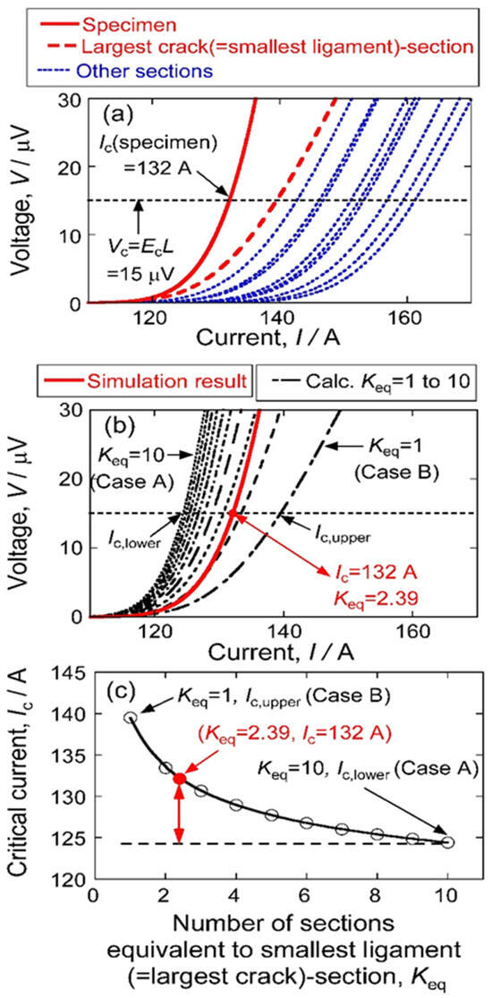
Figure 2.
Relation of the critical current Ic to the number of sections equivalent to the smallest ligament (largest crack) section, Keq, where data of the 15 cm specimen taken from the simulation result are used as an example. In this example specimen, Lp,smallest was 0.617, and Ic was 132 A. (a) V–I curves of the example specimen (solid curve), the smallest ligament section (broken curve), and the other sections (dotted curves). (b) Comparison of the V–I curve of the example specimen (solid curve) with the V–I curves calculated with Keq = 1 to 10. The Keq value, corresponding to Ic = 132 A for Lp,smallest = 0.617 of the example specimen, was estimated to be 2.39. (c) The relation of the Ic value to Keq value for Lp,smallest = 0.617, shows the increase in Ic value from the lower bound (Case A) to the upper bound (Case B) with decreasing Keq from 10 to 1. The location of Ic = 132 A at Keq = 2.39 in the Ic − Keq diagram of the example specimen is shown with the closed circle.
Figure 2b compares the V–I curve of the specimen obtained by simulation and the V–I curves of the specimen calculated with Lp,smallest = 0.617 for Keq = 1 to 10. At V = Vc = 15 μV, the Ic value of the specimen obtained by simulation was 132 A. This value is between the Ic values calculated with Keq = 2 and 3. It is noted that not only the integers but also the decimal places can be used as the Keq value for the calculation of the V–I curve and Ic of the specimen since Equations (8)–(10) hold mathematically for positive real numbers, including decimal places. Using Equations (8)–(10), the Keq value that describes the simulation result of Ic = 132 A at V = Vc = 15 μV for Lp,smallest = 0.617 was 2.39, as shown in Figure 2b.
Figure 2c shows the relation of the Ic value to Keq value for Lp,smallest = 0.617 in 15 cm-specimen, obtained from the V–I curves for Keq = 1 to 10 in Figure 2b. It is shown that the lower bound of critical current Ic,lower corresponding to Keq = 10 in this example, is determined by the effect of Factor 1 (size of the largest crack, which is monitored by Lp,smallest) and the effect of Factor 2 (size difference among cracks, which is monitored by Keq) plays a role in raising Ic from Ic,lower. In this way, the effects of Factor 1 and Factor 2 on Ic could be evaluated separately.
3. Results
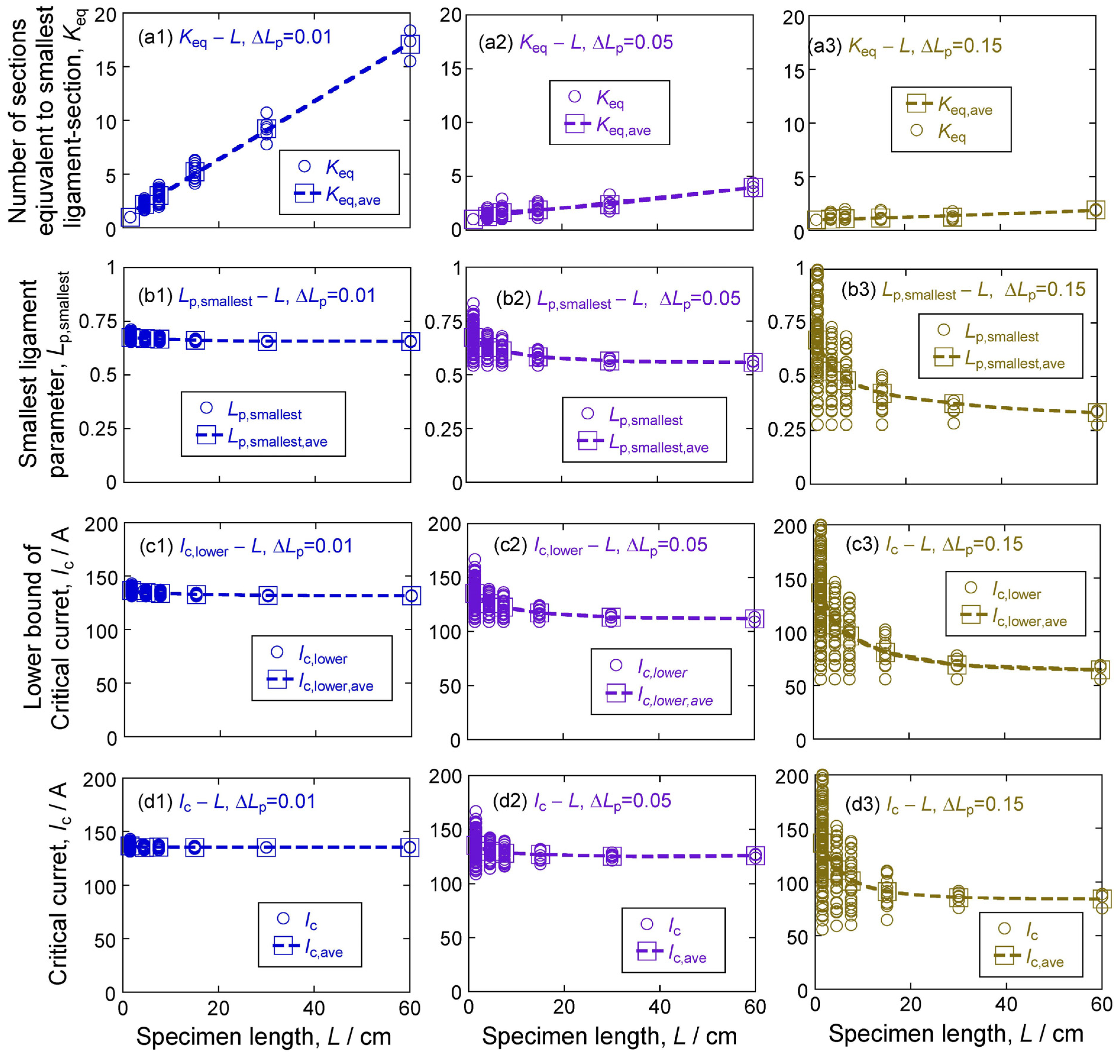
The number of sections equivalent to the smallest ligament section Keq, smallest ligament parameter among all sections Lp,smallest, lower bound of critical current Ic,lower and critical current Ic with an increase in specimen length L (1.5~60 cm) were investigated for a wide standard deviation of ligament parameter values ΔLp = 0.01 to 0.15. Figure 3 shows the plots of Keq, Lp,smallest, Ic,lower, and Ic against L, obtained for ΔLp = 0.01, 0.05, and 0.15. The Keq values were obtained by analysis of the simulation results with the approach in Section 2.2. The Lp,smallest, Ic,lower, and Ic values were obtained by simulation. The value of each specimen is shown with a circle (○) and the average value with a square (□). While the Keq, Lp,smallest, Ic,lower, and Ic values are different from specimen to specimen, the average values (Keq,ave, Lp,smallest,ave, Ic,lower,ave, and Ic,ave) show their correlation to L and ΔLp.
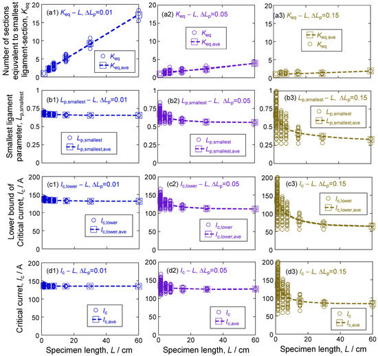
Figure 3.
Plots of number of sections equivalent to the smallest ligament section Keq (a1–a3), smallest ligament parameter Lp,smallest (b1–b3), lower bound of critical current Ic,lower (c1–c3) and critical current Ic (d1–d3), against specimen length L. These data were obtained by simulation and analysis for the standard deviation of the ligament parameter ΔLp = 0.01 (a1–d1), 0.05 (a2–d2), and 0.15 (a3–d3). The value of each specimen is shown with a circle ○, and the average value under the combination pair of L value and ΔLp value is shown with a square □.
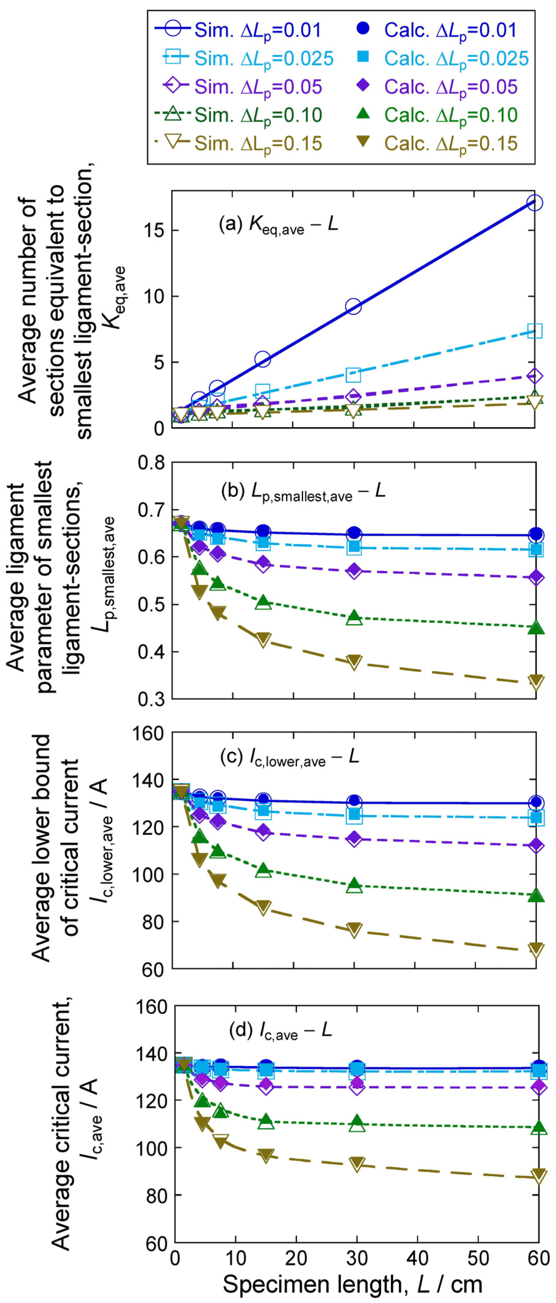
Figure 4 shows the plots of an average of (a) number of sections equivalent to the largest crack section, Keq,ave, (b) smallest ligament parameter, Lp,smallest,ave, (c) lower bound of critical current, Ic,lower,ave, and (d) critical current, Ic,ave, with an increase in L in each case of ΔLp = 0.01, 0.025, 0.05, 0.1, and 0.15. The open symbols for Keq,ave, Lp,smallest,ave, Ic,lower,ave, and Ic,ave, show the results obtained by simulation. The closed symbols in Figure 4b–d show the Lp,smallest,ave, Ic,lower,ave, and Ic,ave values obtained by calculation, whose method is shown in Section 4.1.
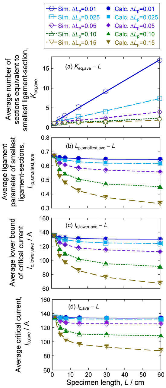
Figure 4.
Changes of the average values of (a) Keq,ave, (b) Lp,smallest,ave, (c) Ic,lower,ave, and (d) Ic,ave, with an increase in specimen length L under the indicated value of ΔLp. The open and closed symbols show the values obtained by simulation and calculation, respectively.
The following features are read in Figure 4:
- The average smallest ligament parameter Lp,smallest,ave decreases with an increase in L. Namely, the average size of the largest crack increases with an increase in L. The extent of the increment of the size of the largest crack with L is enhanced with an increase in ΔLp;
- Average critical current Ic,ave decreases with an increase in specimen length L. The extent of the decrease in Ic,ave with L increases with the increase in the standard deviation of the ligament size (=standard deviation of crack size) ΔLp;
- The change in the average of critical current Ic,ave and the average of the lower bound of critical) current Ic,lower,ave with an increase in specimen length L is similar to the change in Lp,smallest,ave. This result suggests that the decrease in Lp,smallest,ave, namely the increase in the size of the largest crack, has a significant influence on the determination of critical current.
The features mentioned above will be analyzed numerically from the viewpoint of the effects of Factor 1 and Factor 2 on Ic.
4. Discussion
4.1. Calculation of Average Values of the Smallest Ligament Parameter, Lower Bound of Critical Current, Critical Current, and the Correlation between the Smallest Ligament Parameter and Lower Bound of Critical Current
Gumbel’s extreme value distribution function [33] describes the distribution of the extreme values of the smallest ligament (largest crack) parameter Lp,smallest in the present specimens, and the calculation results are compared with the present simulation and analyzed results. The cumulative probability of Lp,smallest value, ϕ (Lp,smallest), and the average Lp,smallest value, Lp,smallest,ave, for each set of ΔLp and L values under the given value of Lp,ave (=0.667 in this work) are expressed as Equations (11)–(14).
Lp,smallest,ave = λ − αγ
λ and α are the positional and scale parameters, respectively, and γ is the Euler–Mascheroni constant (=0.5772). The values of λ and α under given values of L and ΔLp are obtained by using Equation (1) (cumulative distribution function of Lp: F(Lp)) and Equation (2) probability density function Lp: f(Lp)) and the following relational expressions:
F(λ) = 1/N
α = 1/{N f(λ)}
We can calculate Lp,smallest,ave for given values of L and ΔLp with Equations (1), (2), (12)–(14). Then, we can calculate the Vupper,ave–I curve (Case A), which gives the average lower bound for critical current using Equations (9) and (10). From the calculated Vupper,ave–I curve, we can obtain the Ic,lower,ave value for a given combination pair of L value and ΔLp value with the criterion of Ec = 1 μV/cm. By substituting Lp,smallest = Lp,smallest,ave in Equation (9) and Keq value (Figure 4a) in Equation (10) and applying the Ec = 1 μV/cm criterion, we can calculate the Ic,ave values for L = 1.5 to 60 cm and ΔLp = 0.01 to 0.15.
The calculation results (closed symbols) of the average values of Lp,smallest,ave: smallest ligament parameter, Ic,ave: critical current, and Ic,lower,ave: lower bound of critical current in comparison with the simulation results (open symbols) are shown in Figure 4b–d.
The simulation results of Lp,smallest,ave, Ic,lower,ave, and Ic,ave values were described well by calculation. With the estimated valuers above, the effects of Factor 1 and Factor 2 on the specimen length-dependence of critical current can be estimated separately, as shown below.
4.2. Separate Assessment of Effects of Factor 1 and Factor 2 on Specimen Length-Dependence of Critical Current
The changes of the average critical current Ic,ave of specimens with increasing specimen length were described with Factor 1 monitored by Lp,smallest,ave and Factor 2 monitored by Keq,ave, as shown in Figure 4b. It is noted that, as in Figure 4c, the Ic,lower,ave values of the simulation results were well described by calculation using Case A in which all sections have the same Lp,smallest,ave value (Keq = N). In this case, Factor 1 is zero, and hence, this effect does not arise. Namely, the Ic,lower,ave value reflects just Factor 1. Plotting the Ic,lower,ave values in Figure 4c against the corresponding Lp,smallest,ave values in Figure 4b, we have Figure 5. It is clearly shown that the Ic,lower,ave has almost one to one relation to the Lp,smallest,ave for any specimen length L and any crack size difference ΔLp. Using this feature, the effects of Factor 1 and Factor 2 on the specimen length-dependence of critical current can be assessed separately in the following manner:
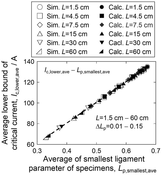
Figure 5.
Plots of average values of the lower bound of critical current Ic,lower,ave against average values of smallest ligament parameter Lp,smallest,ave. The data were taken from the results in Figure 4b,c. The values obtained by simulation and calculation are shown with the open and closed symbols, respectively.
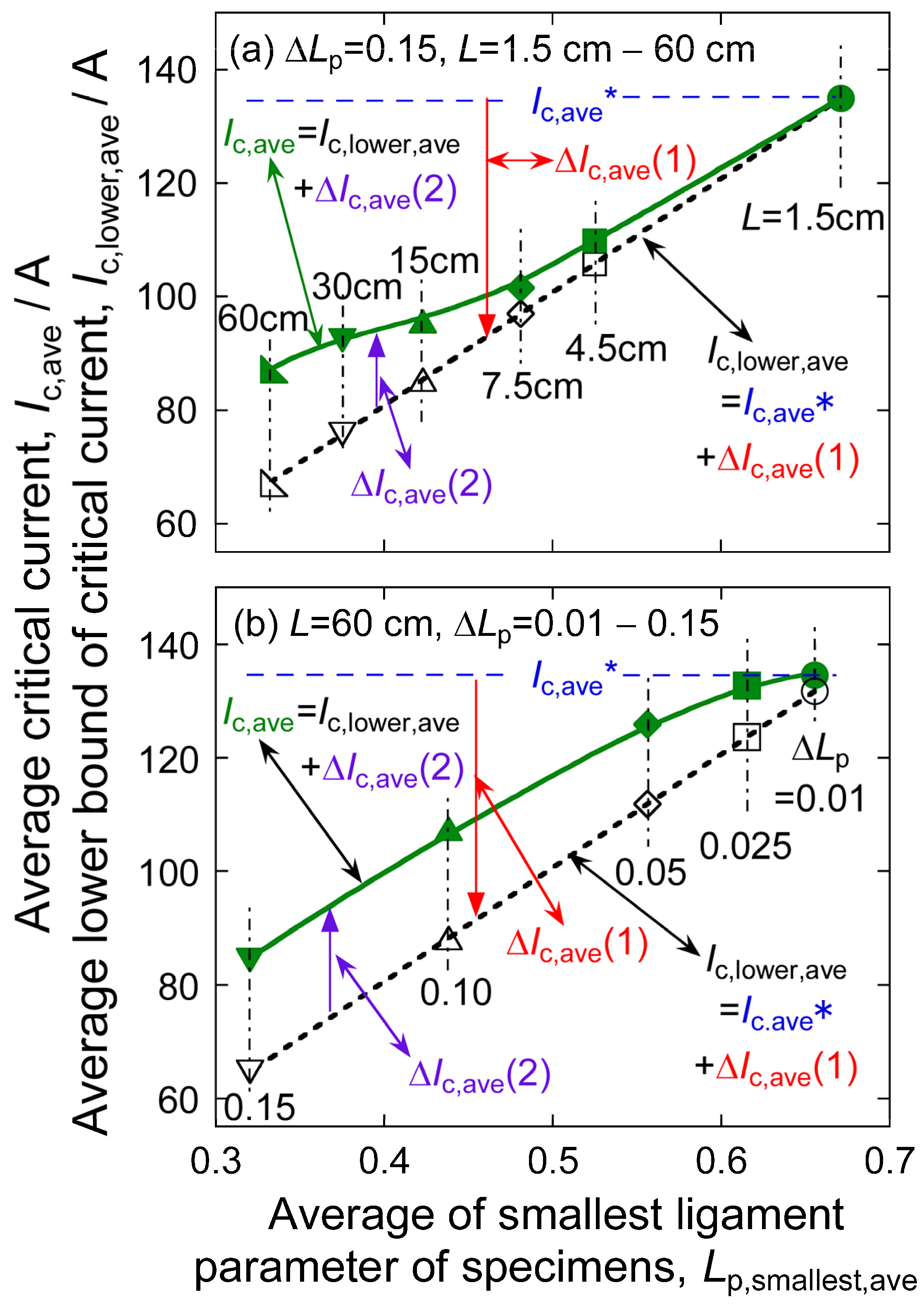
Figure 6 shows the plots of Ic,ave and Ic,lower,ave, obtained by simulation under the condition of (a) ΔLp = 0.15 and L = 1.5 cm to 60 cm, and (b) ΔLp = 0.01 to 0.15 and L = 60 cm, against Lp,smallest,ave. The solid and broken lines show the relations of Ic,ave to Lp,smallest,ave and Ic,lower,ave to Lp,smallest,ave, respectively. The average critical current of the sections for any length is noted as Ic,ave* (=135 A). The value of Ic,ave* = 135 A is equal to the critical current value that appears if uniform cracking takes place under the condition of ΔLp = 0 and Lp,ave = 0.667. This value is kept for any specimen length under ΔLp = 0. The change of critical current ΔIc,ave (1) caused by the increase in Factor 1 and the change of critical current ΔIc,ave (2) caused by the increase in Factor 2 at the critical voltage with increasing L and ΔLp are indicated with arrows.
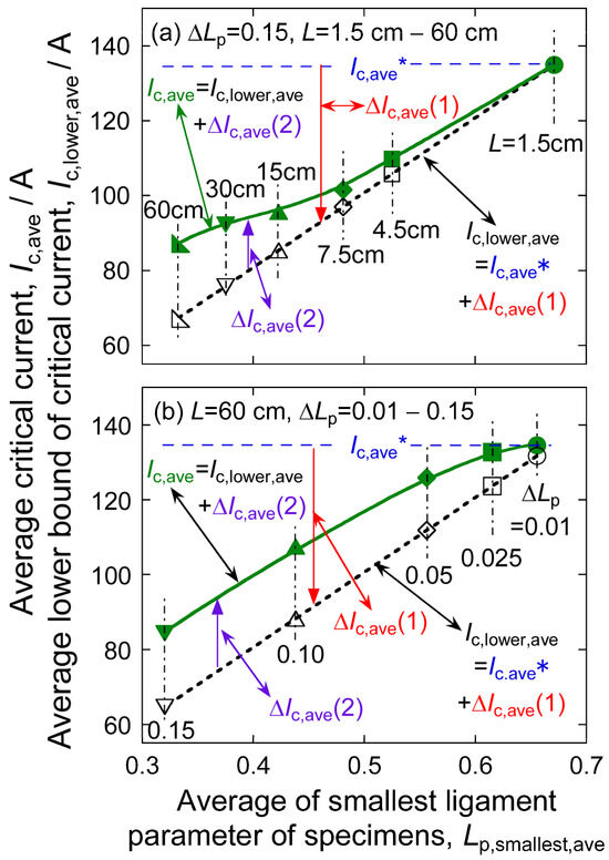
Figure 6.
Plots of average critical current Ic,ave and average lower bound of critical current Ic,lower,ave, obtained by simulation under the condition of (a) standard deviation of the ligament parameter ΔLp = 0.15, and specimen length L = 1.5 cm to 60 cm, and (b) ΔLp = 0.01 to 0.15 and L = 60 cm, against the average smallest ligament parameter Lp,smallest,ave. The relations of Ic,ave to Lp,smallest,ave and Ic,lower,ave to Lp,smallest,ave are presented with the solid and broken lines, respectively. The average critical current of the specimens in the case of ΔLp = 0 is noted as Ic,ave* (=135 A in this work). This value is kept for any specimen length. The change of critical current ΔIc,ave (1) caused by the increase in Factor 1 and the change of critical current ΔIc,ave (2) caused by an increase in Factor 2 are indicated with arrows.
Evidently, with a decreasing average of the smallest ligament parameter Lp,smallest,ave, namely with increasing size of largest crack, values of Ic,ave and Ic,lower,ave decrease, ΔIc,ave (1) increases more in a minus direction caused by decreased Ic,lower,ave, and ΔIc,ave (2) increases caused by an increase of the difference between Ic,ave and Ic,lower,ave. In this way, an increase in specimen length L and an increase in width of crack size distribution ΔLp lead to an increase in Factor 1, which reduces critical current, and an increase in Factor 2, which raises the critical current by ΔIc,ave (2).
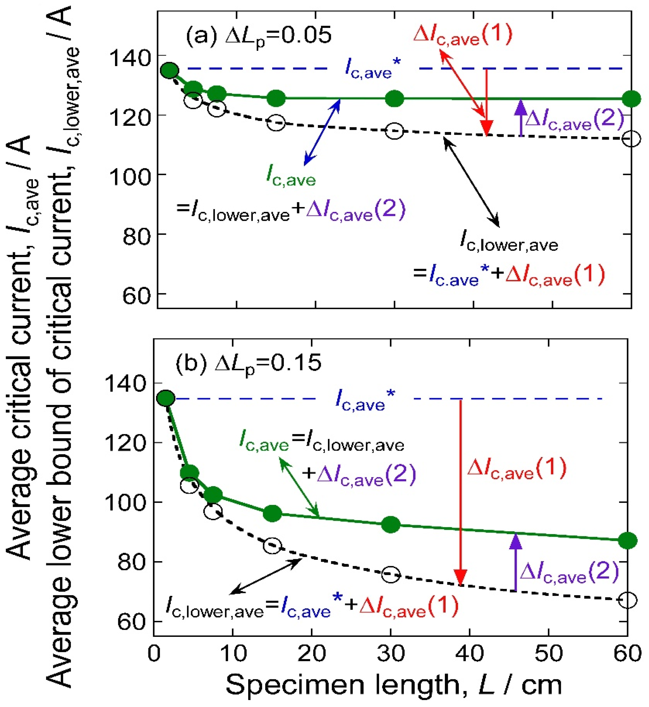
Figure 7 shows Ic,ave, Ic,lower,ave, ΔIc,ave (1) and ΔIc,ave (2) plotted against specimen length L for ΔLp = (a) 0.05 and (b) 0.15. As stated above, if cracking occurs uniformly (ΔLp = 0) as the geometry of Case A (Keq = N), the critical current value does not vary with specimen length, and it is kept to be Ic,ave* (=135 A). In practical specimens, cracking occurs heterogeneously (ΔLp > 0), and hence, the critical current value decreases from the Ic,ave* value with increasing specimen length L and width of crack size distribution ΔLp.
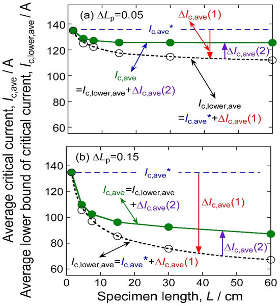
Figure 7.
Changes in average values of critical current Ic,ave and lower bound of critical current Ic,lower,ave with increasing specimen length L in the cases of the standard deviation of ligament parameter ΔLp = (a) 0.05 and (b) 0.15. ΔIc,ave (1) (=Ic,lower,ave − Ic,ave*) refers to the critical current-reducing effect arising from the increase in Factor 1 (size of the largest crack). ΔIc,ave (2) (=Ic,ave − Ic,lower,ave) refers to the critical current-raising effect arising from an increase in Factor 2 (difference in size among cracks).
As shown in Figure 7, with increasing L, the Ic,ave is reduced from Ic,ave* to Ic,lower,ave by ΔIc,ave (1) caused by the effect of increase in Factor 1. The critical current Ic,ave is given by the sum of the Ic,lower,ave, and effect of Factor 2, ΔIc,ave (2), as shown in Figure 2c, Figure 6 and Figure 7. The relations of ΔIc,ave (1) and ΔIc,ave (2) to Ic,ave*, Ic,lower,ave, and Ic,ave, shown in Figure 6 and Figure 7, are expressed below.
The size of the largest crack is different from specimen to specimen. The average size of the largest crack in non-uniform cracking is monitored by Lp,smallest,ave in the present approach, which can be calculated by Equations (12)–(14). Setting Lp,smallest to be equal to the calculated Lp,smallest,ave value and Keq = N in Equations (8)–(10), we can calculate Ic,lower,ave value. We can calculate the Ic,ave values by substituting Lp,smallest = Lp,smallest,ave, and Keq,ave values shown in Figure 4a in Equations (8)–(10). From the value of Ic,ave* = 135 A and the simulated and calculated Ic,lower,ave and Ic,ave values as a function of L for each ΔLp value (0.01~0.15), the ΔIc,ave (1) and ΔIc,ave (2) can be estimated by Equations (15) and (16) from the simulation result and also from the calculation result.
ΔIc,ave (1) = Ic,lower,ave − Ic,ave*
ΔIc,ave (2) = Ic,ave − Ic,lower,ave
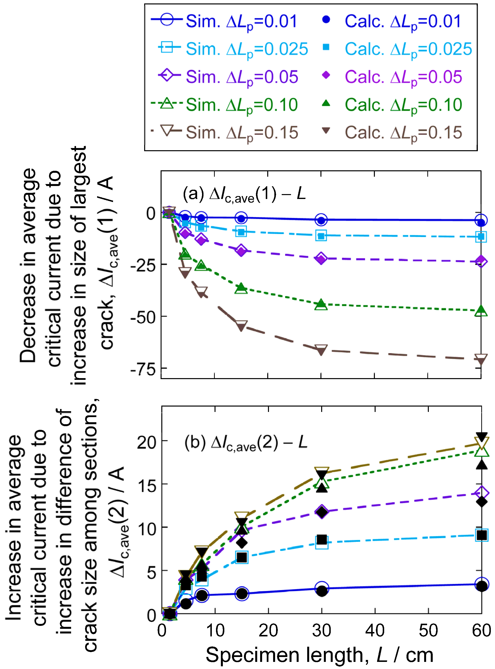
Figure 8 shows specimen length dependence (a) ΔIc,ave (1) and (b) ΔIc,ave (2) for ΔLp = 0.01 to 0.15, estimated by simulation (open symbols) and by calculation (closed symbols). The following features are read:
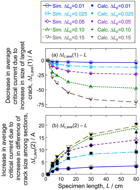
Figure 8.
Estimated specimen length-dependence of the change in average critical current (a) caused by the change of Factor 1, ΔIc,ave (1), and (b) caused by the change of Factor 1, ΔIc,ave (2). The results of simulation and calculation are shown with open and closed symbols, respectively.
- (1)
- ΔIc,ave (1), arising from the increase in the size of the largest crack (Factor 1), increases in minus direction with increasing specimen length L and standard deviation of crack-size distribution ΔLp;
- (2)
- ΔIc,ave (2), arising from the difference in crack size (Factor 2), increases in the plus direction with increasing L and ΔLp;
- (3)
- (4)
- The change in the minus (ΔIc,ave (1))—and plus (ΔIc,ave (2))—effects with specimen length becomes moderate in long specimens.
L is expressed as
Ic,ave = Ic,lower,ave + ΔIc,ave (2) = Ic,ave* + ΔIc,ave (1) + ΔIc,ave (2)
In this work, Ic,ave* is 135 A for any L. Accordingly, whether Ic,ave increases or decreases with increasing L depends on the value of ΔIc,ave (1) + ΔIc,ave (2). Figure 8a,b demonstrates that the Ic,ave decreases with increasing specimen length L since the minus effect ΔIc,ave (1) arising from Factor 1 is larger than the plus effect ΔIc,ave (2) arising from Factor 2.
5. Conclusions
Using a model analysis and a Monte Carlo simulation method, critical current dependence on specimen length was studied by monitoring the effects of Factor 1: size of the largest crack, and Factor 2: size difference among cracks in cracked superconductor. The following results were obtained.
- (1)
- The calculation- and simulation-results showed the following features of the specimen length-dependence of the critical current. (a) Large Factor 1 plays a role in reducing critical current. (b) Large Factor 2 plays a role in raising critical current under a given size of the largest crack. (c) The effect of Factor 1 is larger than that of Factor 2, and hence, the critical current decreases with increasing specimen length. This feature is enhanced with increasing standard deviation of crack size;
- (2)
- For a quantitative description of the results mentioned in (1), the effect of Factor 1 on the critical current of the specimen was formulated by combining the smallest ligament parameter, corresponding to the largest crack section, with a shunting of the current model at the crack. The effect of Factor 2 on critical current was formulated using the number of sections equivalent to the largest crack section at the critical voltage of the specimen’s critical current. With the application of the present approach to the calculation and simulation results, the following results were obtained: (a) The critical current-reducing effect caused by an increase in Factor 1 and the critical current-raising effect caused by the increase in Factor 2 were assessed separately, and the critical current of the specimen was described as a function of specimen length. (b) The features mentioned in (1) were quantitatively described.
Present methods of simulation and calculation are simple, and reliable data are obtained. Thus, the methods and the results in this work are expected to be used for analysis and confirmation of experimental data concerning the relation between critical current, specimen length, and crack size distribution, which provides useful design information to ensure safety and reliability in the practical applications of superconductors.
Author Contributions
Conceptualization, S.O.; Investigation, S.O. and H.O.; Methodology, S.O. and H.O.; Writing—original draft, S.O.; Writing—review & editing, S.O. and H.O. All authors have read and agreed to the published version of the manuscript.
Funding
This research received no external funding.
Institutional Review Board Statement
Not applicable.
Informed Consent Statement
Not applicable.
Data Availability Statement
The data presented in this study are available on request from the corresponding author.
Conflicts of Interest
The authors declare no conflict of interest.
References
- Cheggour, N.; Ekin, J.W.; Thieme, C.H.L.; Xie, Y.-Y.; Selvamanickam, V.; Feenstra, R. Reversible Axial-strain Effect in Y–Ba–Cu–O Coated Conductors. Supercond. Sci. Technol. 2005, 18, S319–S324. [Google Scholar] [CrossRef]
- Van der Laan, D.C.; Ekin, J.W.; Douglas, F.F.; Clickner, C.C.; Stauffer, T.C.; Goodrich, L.F. Effect of Strain, Magnetic Field and Field Angle on the Critical Current Density of YBa2Cu3O7−δ Coated Conductors. Supercond. Sci. Technol. 2010, 23, 072001. [Google Scholar] [CrossRef]
- Ochiai, S.; Arai, T.; Toda, A.; Okuda, H.; Sugano, M.; Osamura, K.; Prusseit, W. Influences of Cracking of Coated Superconducting Layer on Voltage-Current Curve, Critical Current and n-value in DyBCO-Coated Conductor Pulled in Tension. J. Appl. Phys. 2010, 108, 063905. [Google Scholar] [CrossRef]
- Shin, H.S.; Marlon, J.; Dedicatoria, H.; Kim, H.S.; Lee, N.J.; Ha, H.S.; Oh, S.S. Electro-Mechanical Property Investigation of Striated REBCO Coated Conductor Tapes in Pure Torsion Mode. IEEE Trans. Appl. Supercond. 2011, 21, 2997–3000. [Google Scholar] [CrossRef]
- Oguro, H.; Suwa, T.; Suzuki, T.; Awaji, S.; Watanabe, K.; Sugano, M.; Machiya, S.; Sato, T.; Koganezawa, T.; Machi, T.; et al. Relation between the Crystal Axis and the Strain Dependence of Critical Curren under Tensile Strain for GdBCO Coated Conductors. IEEE Trans. Appl. Supercond. 2013, 23, 8400304. [Google Scholar] [CrossRef]
- Zhao, Y.; Ji, P. Crack-Inclusion Problem in a Superconducting Cylinder with Exponential Distribution of Critical Current Density. J. Supercond. Nov. Magn. 2020, 33, 2907–2912. [Google Scholar] [CrossRef]
- Gannon, J.J.; Malozemoff, A.P.; Diehl, R.C.; Antaya, P.; Mori, A. Effect of Length Scale on Critical Current Measurement in High Temperature Superconductor Wires. IEEE Trans. Appl. Supercond. 2013, 23, 8002005. [Google Scholar] [CrossRef]
- Ma, J.; Gao, Y. Numerical Analysis of the Mechanical and Electrical Properties of (RE)BCO Tapes with Multiple Edge Cracks. Supercond. Sci. Technol. 2023, 36, 095013. [Google Scholar] [CrossRef]
- Jiang, Z.; Huang, Y.; Jiang, D.; Chen, W.; Kuang, G. Influence of Edge Crack Propagation on Critical Current Degradation of REBCO Tape Studied by Phase-Field Fracture Method and Current Shunting Model. IEEE Trans. Appl. Supercond. 2023, 33, 8400111. [Google Scholar] [CrossRef]
- Yong, D.; Yang, Y.; Zhou, Y.H. Dynamic Fracture Behavior of a Crack in the Bulk Superconductor under Electromagnetic Force. Eng. Frac. Mech. 2016, 158, 167–178. [Google Scholar] [CrossRef]
- Feng, W.J.; Zhang, R.; Ding, H.M. Crack Problem for an Inhomogeneous Orthotropic Superconducting Slab under an Electromagnetic Force. Phys. C Supercond. 2012, 477, 32–36. [Google Scholar] [CrossRef]
- Gao, P.; Mao, J.; Chen, J.; Wang, X.; Zhou, Y. Electromechanical Degradation of REBCO Coated Conductor Tapes under Combined Tension and Torsion Loading. Int. J. Mech. Sci. 2020, 223, 107314. [Google Scholar] [CrossRef]
- Ochiai, S.; Okuda, O.; Fujii, N. Features of Crack Size Distribution- and Voltage Probe Spacing-Depend ences of Critical Current and n-Value in Cracked Superconducting Tape, Depicted by Simulation. Mater. Trans. 2018, 59, 1628–1636. [Google Scholar] [CrossRef]
- Ochiai, S.; Okuda, H. Effects of Size of the Largest Crack and Size Difference among Cracks on Critical Current of Superconducting Tape with Multiple Cracks in Superconducting Layer. Mater. Trans. 2020, 61, 766–775. [Google Scholar] [CrossRef]
- Akdemir, E.; Pakdil, M.; Bilge, H.; Kahraman, M.F.; Yildirim, G.; Bekiroglu, E.; Zalaoglu, Y.; Doruk, E.; Oz, M. Degeneration of Mechanical Characteristics and Performances with Zr Nanoparticles Inserted in Bi-2223 Superconducting Matrix and Increment in Dislocation Movement and Cracks Propagation. J. Mater. Sci. Mater Electron. 2016, 27, 2276–2287. [Google Scholar] [CrossRef]
- Shigue, C.Y.; Baldan, C.A.; Oliveira, U.R.; Carvalho, F.J.H.; Filho, E.R. Critical Current Degradation of Bi-2223 Composite Tapes Induced by Cyclic Deformation and Fatigue-Related Effects. IEEE Trans. Appl. Supercond. 2006, 16, 1027–1030. [Google Scholar] [CrossRef]
- Fang, Y.; Danyluk, S.; Lanagan, M.T. Effects of Cracks on Critical Current Density in Ag-sheathed Superconductor Tape. Cryogenics 1996, 36, 957–962. [Google Scholar] [CrossRef]
- Van Eck, H.J.M.; Vargas, L.; ten Haken, B.; ten Kate, H.H.J. Bending and Axial Strain Dependence of the Critical Current in Superconducting BSCCO Tapes. Supercond. Sci. Technol. 2002, 15, 1213. [Google Scholar] [CrossRef]
- Gao, P.; Wang, X. Theory Analysis of Critical Current Degeneration in Bended Superconducting Tapes of Multifiment Composite Bi2223/Ag. Phys. C 2015, 517, 31–36. [Google Scholar] [CrossRef]
- Ochiai, S.; Okuda, H.; Sugano, M.; Hojo, M.; Osamura, K. Prediction of Variation in Critical Current with Applied Tensile/Bending Strain of Bi2223 Composite Tape from Tensile Stress-Strain Curve. J. Appl. Phys. 2010, 107, 083904. [Google Scholar] [CrossRef]
- Kitaguchi, H.; Matsumoto, A.; Hatakeyama, H.; Kumakura, H. V–I Characteristics of MgB2 PIT CopositeTapes: N-Values under Strain, in High Fields, or at High Temperatures. Phys. C Supercond. 2004, 401, 246–250. [Google Scholar] [CrossRef]
- Murakami, A.; Iwamoto, A.; Noudem, J.G. Mechanical Properties of Bulk MgB2 Superconductors Processed by Spark Plasma Sintering at Various Temperatures. IEEE Trans. Appl. Supercond. 2018, 28, 8400204. [Google Scholar] [CrossRef]
- Nishijima, G.; Ye, S.J.; Matsumoto, A.; Togano, K.; Kumakura, H.; Kitaguchi, H.; Oguro, H. Mechanical Properties of MgB2 Superconducting Wires Fabricated by Internal Mg Diffusion Process. Supercond. Sci. Technol. 2012, 25, 054012. [Google Scholar] [CrossRef]
- Krinitsina, T.P.; Kuznetsova, E.I.; Degtyarev, M.V.; Blinova, Y.V. MgB2-Based Superconductors: Structure and Properties. Phys. Metals Metallogr. 2021, 122, 1183–1206. [Google Scholar] [CrossRef]
- Alknes, P.; Hagner, M.; Bjoerstad, R.; Scheuerlein, C.; Bordini, B.; Sugano, M.; Hudspeth, J.; Ballarino, A. Mechanical Properties and Strain Induced Filament Degradation of Ex-Situ and In-Situ MgB2 wires. IEEE Trans. Appl. Supercond. 2016, 26, 8401205. [Google Scholar] [CrossRef]
- Miyoshi, Y.; Van Lanen, E.P.A.; Dhallé, M.M.; Nijhuits, N. Distinct Voltage–Current Characteristics of Nb3Sn Strands with Dispersed and Collective Crack Distributions. Supercond. Sci. Technol. 2009, 22, 1085009. [Google Scholar] [CrossRef]
- Feng, Y.; Yong, H.; Zhou, Y. Efficient Multiscale Investigation of Mechanical Behavior in Nb3Sn Superconducting Accelerator Magnet Based on Self-consistent Clustering Analysis. Comp. Struct. 2023, 324, 117541. [Google Scholar] [CrossRef]
- Lenoir, G.; Manil, P.; Nunio, F.; Aubin, V. Mechanical Behavior Laws for Multiscale Numerical Model of Nb3Sn Conductors. IEEE Trans. Appl. Supercond. 2019, 29, 8401706. [Google Scholar] [CrossRef]
- Sheth, M.K.; Lee, P.; McRae, D.M.; Walsh, R.; Starch, W.L.; Jewell, M.C.; Devred, A.; Larbalestier, D.C. Procedures for Evaluating Filament Cracking during Fatigue Testing of Nb3Sn Strand. AIP Conf. Proc. 2012, 1435, 201–208. [Google Scholar] [CrossRef]
- Ta, W.; Li, Y.; Gao, Y. A 3D Model on the Electromechanical Behavior of a Multifilament Twisted Nb3Sn Super conducting Strand. J. Supercond. Nov. Magn. 2015, 28, 2683–2695. [Google Scholar] [CrossRef]
- Zhang, Z.; Sh, L. Elastic–Plastic Mechanical Behavior Analysis of a Nb3Sn Superconducting Strand with Initial Thermal Damage. Appl. Sci. 2022, 12, 8313. [Google Scholar] [CrossRef]
- Nakamura, T.; Takamura, Y.; Amemiya, N.; Nakao, K.; Izumi, T. Longitudinal Inhomogeneity of DC Current Transport Properties in Gd-system HTS Tapes—Statistical Approach for System Design. Cryogenics 2014, 63, 17–24. [Google Scholar] [CrossRef]
- Gumbel, E.J. Statistics of Extremes; Columbia University Press: New York, NY, USA, 1958. [Google Scholar] [CrossRef]


Disclaimer/Publisher’s Note: The statements, opinions and data contained in all publications are solely those of the individual author(s) and contributor(s) and not of MDPI and/or the editor(s). MDPI and/or the editor(s) disclaim responsibility for any injury to people or property resulting from any ideas, methods, instructions or products referred to in the content. |
© 2023 by the authors. Licensee MDPI, Basel, Switzerland. This article is an open access article distributed under the terms and conditions of the Creative Commons Attribution (CC BY) license (https://creativecommons.org/licenses/by/4.0/).