
Time–Temperature Superposition of the Dissolution of Wool Yarns in the Ionic Liquid 1-Ethyl-3-methylimidazolium Acetate


Abstract
1. Introduction
2. Materials and Methods
2.1. Materials
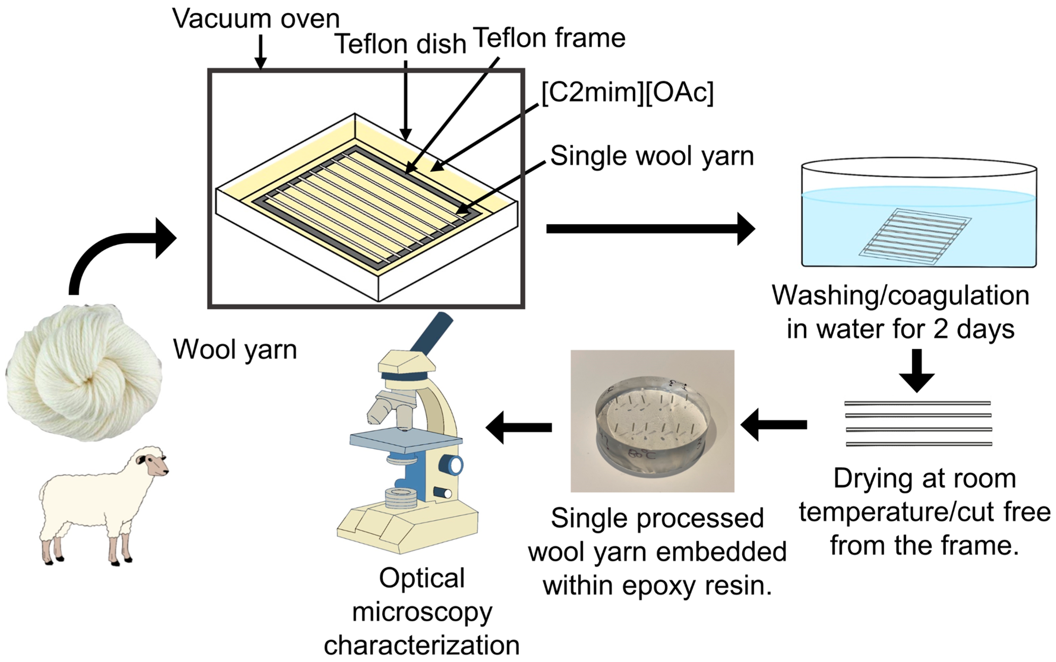
2.2. Sample Preparation
2.3. Optical Microscopy
2.4. Modelling Thickness Loss of Dissolved Wool Yarn
3. Results and Discussion
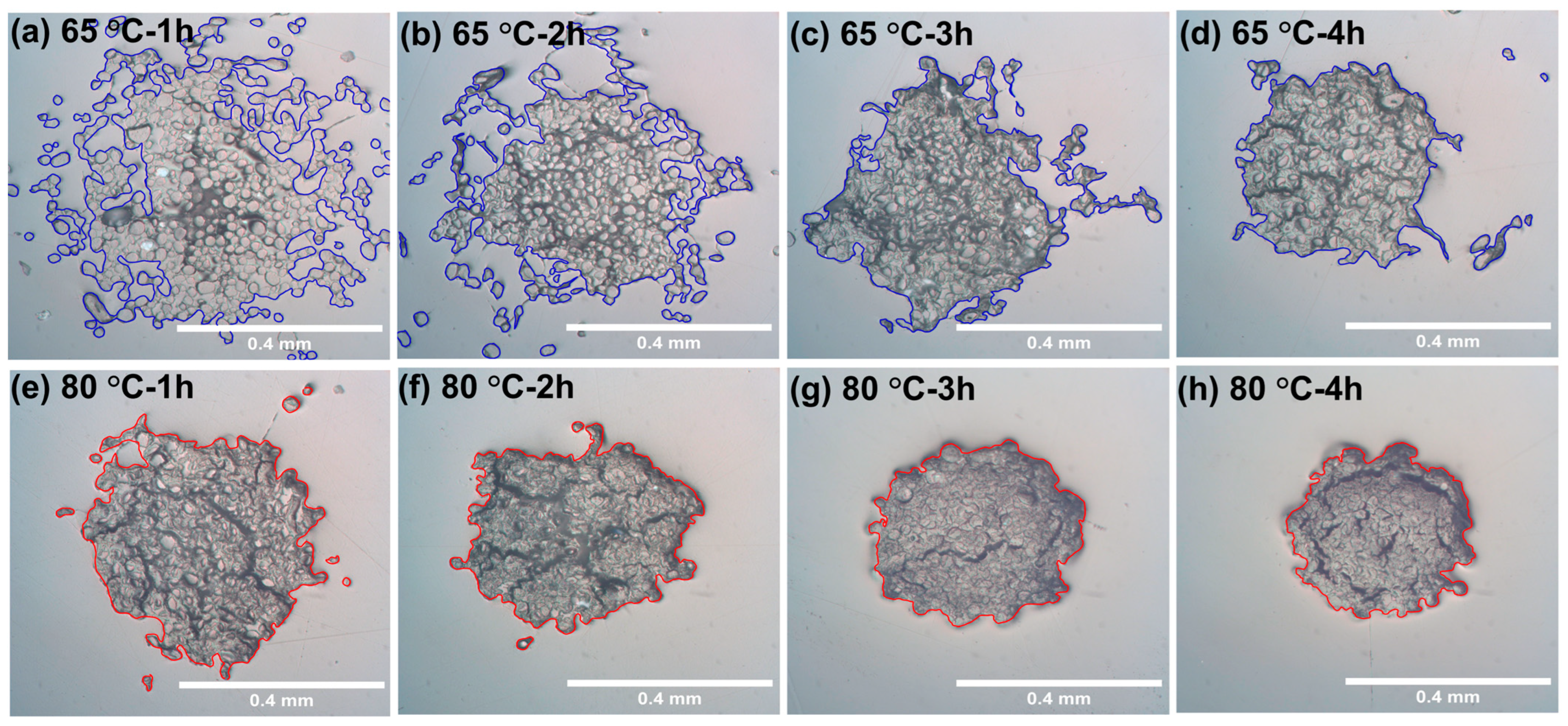
3.1. Optical Microscopy
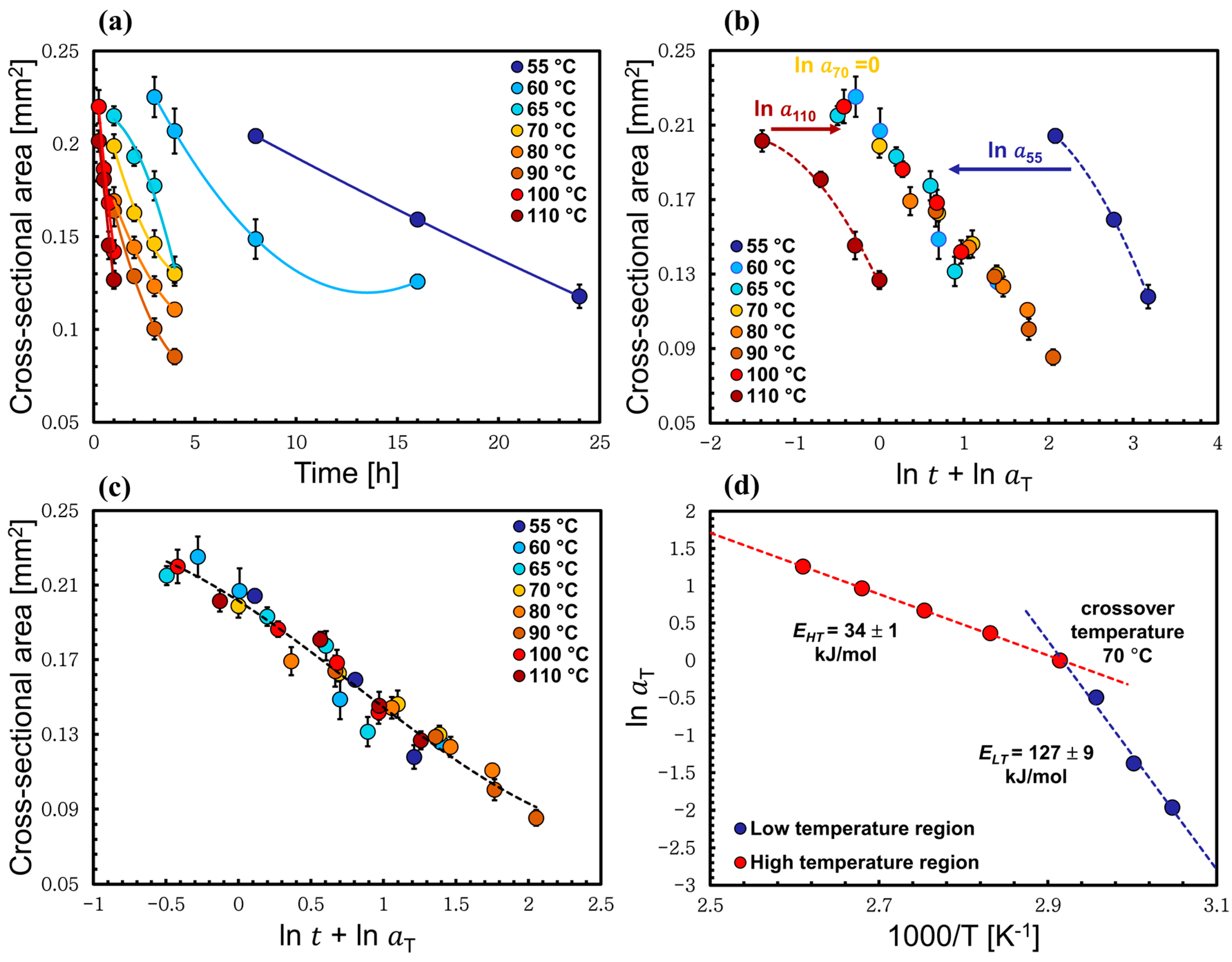
3.2. Time–Temperature Superposition Method Applied to Low-Temperature Process
3.3. Time–Temperature Superposition Method Applied to High-Temperature Process
3.4. Method to Calculate the Self-Diffusion Coefficient through the Thickness Loss of the Wool Yarn
4. Conclusions
Supplementary Materials
Author Contributions
Funding
Institutional Review Board Statement
Informed Consent Statement
Data Availability Statement
Acknowledgments
Conflicts of Interest
References
- Mohammed, L.; Ansari, M.N.M.; Pua, G.; Jawaid, M.; Islam, M.S. A Review on Natural Fiber Reinforced Polymer Composite and Its Applications. Int. J. Polym. Sci. 2015, 2015, 243947. [Google Scholar] [CrossRef]
- Balaji, A.B.; Pakalapati, H.; Khalid, M.; Walvekar, R.; Siddiqui, H. Natural and synthetic biocompatible and biodegradable polymers. Biodegrad. Biocompatible Polym. Compos. 2018, 286, 3–32. [Google Scholar] [CrossRef]
- Yadav, P.; Yadav, H.; Shah, V.G.; Shah, G.; Dhaka, G. Biomedical biopolymers, their origin and evolution in biomedical sciences: A systematic review. J. Clin. Diagn. Res. JCDR 2015, 9, ZE21. [Google Scholar] [CrossRef]
- Zhang, Z.; Nie, Y.; Zhang, Q.; Liu, X.; Tu, W.; Zhang, X.; Zhang, S. Quantitative Change in Disulfide Bonds and Microstructure Variation of Regenerated Wool Keratin from Various Ionic Liquids. ACS Sustain. Chem. Eng. 2017, 5, 2614–2622. [Google Scholar] [CrossRef]
- Ham, T.R.; Lee, R.T.; Han, S.; Haque, S.; Vodovotz, Y.; Gu, J.; Burnett, L.R.; Tomblyn, S.; Saul, J.M. Tunable Keratin Hydrogels for Controlled Erosion and Growth Factor Delivery. Biomacromolecules 2016, 17, 225–236. [Google Scholar] [CrossRef]
- Eslahi, N.; Dadashian, F.; Nejad, N.H. An Investigation on Keratin Extraction from Wool and Feather Waste by Enzymatic Hydrolysis. Prep. Biochem. Biotechnol. 2013, 43, 624–648. [Google Scholar] [CrossRef]
- Zoccola, M.; Aluigi, A.; Tonin, C. Characterisation of keratin biomass from butchery and wool industry wastes. J. Mol. Struct. 2009, 938, 35–40. [Google Scholar] [CrossRef]
- Cardamone, J.M.; Nuñez, A.; Garcia, R.A.; Aldema-Ramos, M. Characterizing Wool Keratin. Res. Lett. Mater. Sci. 2009, 2009, 147175. [Google Scholar] [CrossRef]
- Wang, D.; Tang, R.-C. Dissolution of wool in the choline chloride/oxalic acid deep eutectic solvent. Mater. Lett. 2018, 231, 217–220. [Google Scholar] [CrossRef]
- Chou, C.-C.; Buehler, M.J. Structure and Mechanical Properties of Human Trichocyte Keratin Intermediate Filament Protein. Biomacromolecules 2012, 13, 3522–3532. [Google Scholar] [CrossRef]
- Jiang, Z.; Yuan, J.; Wang, P.; Fan, X.; Xu, J.; Wang, Q.; Zhang, L. Dissolution and regeneration of wool keratin in the deep eutectic solvent of choline chloride-urea. Int. J. Biol. Macromol. 2018, 119, 423–430. [Google Scholar] [CrossRef]
- Idris, A.; Vijayaraghavan, R.; Rana, U.A.; Patti, A.F.; MacFarlane, D.R. Dissolution and regeneration of wool keratin in ionic liquids. Green Chem. 2014, 16, 2857–2864. [Google Scholar] [CrossRef]
- Fraser, R.; MacRae, T.; Rogers, G.E. Keratins: Their Composition, Structure and Biosynthesis; Charles C Thomas Publisher: Springfield, IL, USA, 1972. [Google Scholar]
- Barone, J.R.; Schmidt, W.F.; Liebner, C.F. Thermally processed keratin films. J. Appl. Polym. Sci. 2005, 97, 1644–1651. [Google Scholar] [CrossRef]
- Feroz, S.; Muhammad, N.; Dias, G.; Alsaiari, M.A. Extraction of keratin from sheep wool fibres using aqueous ionic liquids assisted probe sonication technology. J. Mol. Liq. 2022, 350, 118595. [Google Scholar] [CrossRef]
- Alemdar, A.; Iridag, Y.; Kazanci, M. Flow behavior of regenerated wool-keratin proteins in different mediums. Int. J. Biol. Macromol. 2005, 35, 151–153. [Google Scholar] [CrossRef]
- Donato, R.K.; Mija, A. Keratin Associations with Synthetic, Biosynthetic and Natural Polymers: An Extensive Review. Polymers 2019, 12, 32. [Google Scholar] [CrossRef]
- Vasconcelos, A.; Freddi, G.; Cavaco-Paulo, A. Biodegradable Materials Based on Silk Fibroin and Keratin. Biomacromolecules 2008, 9, 1299–1305. [Google Scholar] [CrossRef]
- Shavandi, A.; Silva, T.H.; Bekhit, A.A.; Bekhit, A.E.-D.A. Keratin: Dissolution, extraction and biomedical application. Biomater. Sci. 2017, 5, 1699–1735. [Google Scholar] [CrossRef]
- Meng, Z.; Zheng, X.; Tang, K.; Liu, J.; Qin, S. Dissolution of natural polymers in ionic liquids: A review. e-Polymers 2012, 12, 28. [Google Scholar] [CrossRef]
- Mahmood, H.; Moniruzzaman, M.; Yusup, S.; Welton, T. Ionic liquids assisted processing of renewable resources for the fabrication of biodegradable composite materials. Green Chem. 2017, 19, 2051–2075. [Google Scholar] [CrossRef]
- Yang, X.; Qiao, C.; Li, Y.; Li, T. Dissolution and resourcfulization of biopolymers in ionic liquids. React. Funct. Polym. 2016, 100, 181–190. [Google Scholar] [CrossRef]
- Niedermeyer, H.; Hallett, J.P.; Villar-Garcia, I.J.; Hunt, P.A.; Welton, T. Mixtures of ionic liquids. Chem. Soc. Rev. 2012, 41, 7780–7802. [Google Scholar] [CrossRef]
- Xie, H.; Li, S.; Zhang, S. Ionic liquids as novel solvents for the dissolution and blending of wool keratin fibers. Green Chem. 2005, 7, 606–608. [Google Scholar] [CrossRef]
- Swatloski, R.P.; Spear, S.K.; Holbrey, J.D.; Rogers, R.D. Dissolution of Cellose with Ionic Liquids. J. Am. Chem. Soc. 2002, 124, 4974–4975. [Google Scholar] [CrossRef]
- Phillips, D.M.; Drummy, L.F.; Conrady, D.G.; Fox, D.M.; Naik, R.R.; Stone, M.O.; Trulove, P.C.; De Long, H.C.; Mantz, R.A. Dissolution and Regeneration of Bombyx mori Silk Fibroin Using Ionic Liquids. J. Am. Chem. Soc. 2004, 126, 14350–14351. [Google Scholar] [CrossRef]
- Liu, X.; Nie, Y.; Meng, X.; Zhang, Z.; Zhang, X.; Zhang, S. DBN-based ionic liquids with high capability for the dissolution of wool keratin. RSC Adv. 2017, 7, 1981–1988. [Google Scholar] [CrossRef]
- Shavandi, A.; Jafari, H.; Zago, E.; Hobbi, P.; Nie, L.; De Laet, N. A sustainable solvent based on lactic acid and l-cysteine for the regeneration of keratin from waste wool. Green Chem. 2021, 23, 1171–1174. [Google Scholar] [CrossRef]
- Giteru, S.G.; Ramsey, D.H.; Hou, Y.; Cong, L.; Mohan, A.; Bekhit, A.E.D.A. Wool keratin as a novel alternative protein: A comprehensive review of extraction, purification, nutrition, safety, and food applications. Compr. Rev. Food Sci. Food Saf. 2023, 22, 643–687. [Google Scholar] [CrossRef]
- Smith, E.L.; Abbott, A.P.; Ryder, K.S. Deep Eutectic Solvents (DESs) and Their Applications. Chem. Rev. 2014, 114, 11060–11082. [Google Scholar] [CrossRef]
- Chen, J.; Vongsanga, K.; Wang, X.; Byrne, N. What Happens during Natural Protein Fibre Dissolution in Ionic Liquids. Materials 2014, 7, 6158–6168. [Google Scholar] [CrossRef]
- Lovell, C.S.; Walker, A.; Damion, R.A.; Radhi, A.; Tanner, S.F.; Budtova, T.; Ries, M.E. Influence of Cellulose on Ion Diffusivity in 1-Ethyl-3-Methyl-Imidazolium Acetate Cellulose Solutions. Biomacromolecules 2010, 11, 2927–2935. [Google Scholar] [CrossRef]
- Green, S.M.; Ries, M.E.; Moffat, J.; Budtova, T. NMR and Rheological Study of Anion Size Influence on the Properties of Two Imidazolium-based Ionic Liquids. Sci. Rep. 2017, 7, 8968. [Google Scholar] [CrossRef]
- Ries, M.E.; Radhi, A.; Keating, A.S.; Parker, O.; Budtova, T. Diffusion of 1-Ethyl-3-methyl-imidazolium Acetate in Glucose, Cellobiose, and Cellulose Solutions. Biomacromolecules 2014, 15, 609–617. [Google Scholar] [CrossRef]
- Cuadrado-Prado, S.; Domínguez-Pérez, M.; Rilo, E.; García-Garabal, S.; Segade, L.; Franjo, C.; Cabeza, O. Experimental measurement of the hygroscopic grade on eight imidazolium based ionic liquids. Fluid Phase Equilibria 2009, 278, 36–40. [Google Scholar] [CrossRef]
- Hawkins, J.E.; Liang, Y.; Ries, M.E.; Hine, P.J. Time temperature superposition of the dissolution of cellulose fibres by the ionic liquid 1-ethyl-3-methylimidazolium acetate with cosolvent dimethyl sulfoxide. Carbohydr. Polym. Technol. Appl. 2021, 2, 100021. [Google Scholar] [CrossRef]
- Liang, Y.; Hawkins, J.E.; Ries, M.E.; Hine, P.J. Dissolution of cotton by 1-ethyl-3-methylimidazolium acetate studied with time–temperature superposition for three different fibre arrangements. Cellulose 2021, 28, 715–727. [Google Scholar] [CrossRef]
- Ferry, J.D. Viscoelastic Properties of Polymers; John Wiley & Sons: Hoboken, NJ, USA, 1980. [Google Scholar]
- Zhang, X.; Ries, M.E.; Hine, P.J. Time–Temperature Superposition of the Dissolution of Silk Fibers in the Ionic Liquid 1-Ethyl-3-methylimidazolium Acetate. Biomacromolecules 2021, 22, 1091–1101. [Google Scholar] [CrossRef]
- Laidler, K.J. The development of the Arrhenius equation. J. Chem. Educ. 1984, 61, 494. [Google Scholar] [CrossRef]
- Aakeröy, C.B.; Seddon, K.R. The hydrogen bond and crystal engineering. Chem. Soc. Rev. 1993, 22, 397–407. [Google Scholar] [CrossRef]
- Sunner, S.; Ballhausen, C.; Bjerrum, J.; Clauson-Kaas, N. Thermochemical Investigation on Organic Sulfur Compounds. IV. Thermochemical Sulfur Bond Energy Terms. Acta Chem. Scand. 1955, 9, 837–846. [Google Scholar] [CrossRef]
- Kim, S.; Wittek, K.I.; Lee, Y. Synthesis of poly (disulfide) s with narrow molecular weight distributions via lactone ring-opening polymerization. Chem. Sci. 2020, 11, 4882–4886. [Google Scholar] [CrossRef] [PubMed]
- Bin Rusayyis, M.A.; Torkelson, J.M. Reprocessable covalent adaptable networks with excellent elevated-temperature creep resistance: Facilitation by dynamic, dissociative bis(hindered amino) disulfide bonds. Polym. Chem. 2021, 12, 2760–2771. [Google Scholar] [CrossRef]


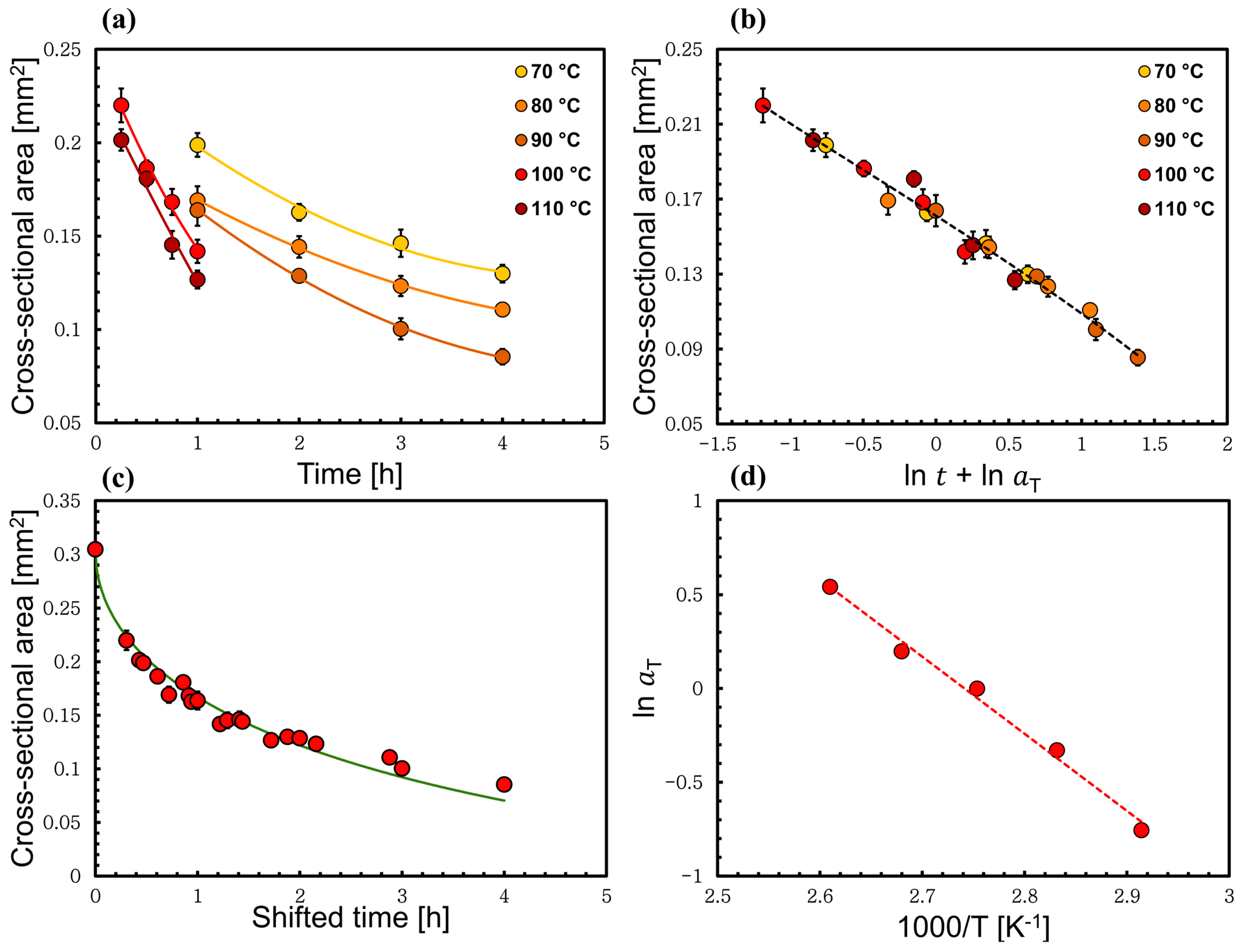
| T Crossover (°C) | ELT (kJ/mol) | EHT (kJ/mol) | Regression Coefficient R2 |
|---|---|---|---|
| 65 | 128 ± 20 | 41 ± 4 | 0.9741 |
| 70 | 127 ± 9 | 34 ± 1 | 0.9946 |
| 80 | 143 ± 16 | 39 ± 1 | 0.9569 |
| 90 | 139 ± 14 | 37 ± 7 | 0.9137 |
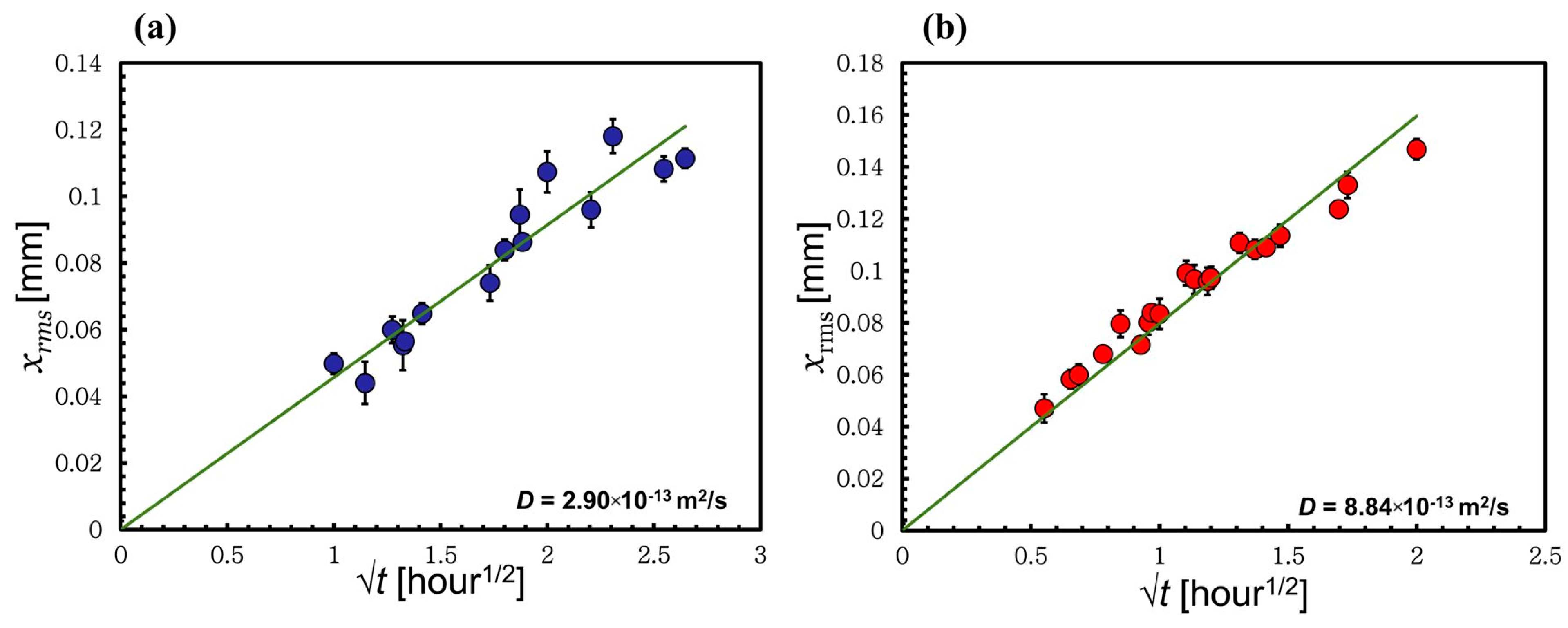
| Reference Temperature (°C) | D[C2mim][OAc] (10−13m2s−1) |
|---|---|
| 55 | 0.64 |
| 60 | 1.27 |
| 65 | 2.90 |
| 70 | 4.74 |
| Reference Temperature (°C) | D[C2mim][OAc] (10−13m2s−1) |
|---|---|
| 80 | 6.33 |
| 90 | 8.84 |
| 100 | 11.50 |
| 110 | 15.31 |
Disclaimer/Publisher’s Note: The statements, opinions and data contained in all publications are solely those of the individual author(s) and contributor(s) and not of MDPI and/or the editor(s). MDPI and/or the editor(s) disclaim responsibility for any injury to people or property resulting from any ideas, methods, instructions or products referred to in the content. |
© 2024 by the authors. Licensee MDPI, Basel, Switzerland. This article is an open access article distributed under the terms and conditions of the Creative Commons Attribution (CC BY) license (https://creativecommons.org/licenses/by/4.0/).
Share and Cite
Alghamdi, A.S.; Hine, P.J.; Ries, M.E. Time–Temperature Superposition of the Dissolution of Wool Yarns in the Ionic Liquid 1-Ethyl-3-methylimidazolium Acetate. Materials 2024, 17, 244. https://doi.org/10.3390/ma17010244
Alghamdi AS, Hine PJ, Ries ME. Time–Temperature Superposition of the Dissolution of Wool Yarns in the Ionic Liquid 1-Ethyl-3-methylimidazolium Acetate. Materials. 2024; 17(1):244. https://doi.org/10.3390/ma17010244
Chicago/Turabian StyleAlghamdi, Amjad Safar, Peter John Hine, and Michael Edward Ries. 2024. "Time–Temperature Superposition of the Dissolution of Wool Yarns in the Ionic Liquid 1-Ethyl-3-methylimidazolium Acetate" Materials 17, no. 1: 244. https://doi.org/10.3390/ma17010244
APA StyleAlghamdi, A. S., Hine, P. J., & Ries, M. E. (2024). Time–Temperature Superposition of the Dissolution of Wool Yarns in the Ionic Liquid 1-Ethyl-3-methylimidazolium Acetate. Materials, 17(1), 244. https://doi.org/10.3390/ma17010244