
Residual Stresses in Ribbed Reinforcing Bars


Abstract
:1. Introduction
2. Theory
2.1. Tempering of Martensite
- Stage 1: precipitation of -iron carbide (Fe2.4C) and partial loss of tetragonality via diffusion of carbon atoms to dislocations and grain boundaries;
- Stage 2: decomposition of retained austenite;
- Stage 3: dissolution of the -iron carbides formed in stage 1, formation of cementite (Fe3C) and full loss of tetragonality in martensite;
- Stage 4: coarsening and spheroidization of cementite and recrystallization of ferrite.
2.2. Transformation-Induced Plasticity
2.3. Residual Stress Measurements on Rebars
- On the surface of a rebar with a diameter of mm, Hameed et al. [11] determined compressive axial and compressive tangential residual stresses of about −10 MPa and −40 MPa, respectively, between alternating ribs. At a depth of 0.3 mm below the rebar surface, Hameed et al. [11] determined axial and tangential compressive residual stresses of about −90 MPa and about −105 MPa, respectively. For the residual stress measurements, Hameed et al. [11] used an X-ray diffraction technique.
- On the surface of rebars with diameters of mm, Zheng et al. [8] determined axial compressive residual stresses between −80 MPa and −90 MPa by using a cut-compliance method.
- Volkwein et al. [7] determined axial compressive residual stresses of approximately MPa on the surface of a first rebar with a diameter of mm. On the surface of a second rebar with the same diameter, which was produced by a different manufacturer, they determined axial tensile residual stresses of approximately 10 MPa. In the transition zone, Volkwein et al. [7] determined tensile residual stresses of approximately 45 MPa and 40 MPa, respectively. In the core, the authors determined compressive residual stresses of approximately MPa and MPa, respectively. For the residual stress measurements, Volkwein et al. [7] used a cut-compliance method. At first, the authors partitioned the rebar specimens each into two outer segments and one middle segment (see Figure 2). Then, they carried out the residual stress measurements only on the middle segment.
- Rocha et al. [9] measured axial compressive residual stresses in the non-ribbed region of the surface of a rebar with a diameter of mm. Between alternating ribs, they determined axial compressive residual stresses within the range of −48 MPa to −147 MPa and between parallel ribs within the range of −26 MPa to −61 MPa. At a depth of 0.05 mm, Rocha et al. [9] measured axial tensile residual stresses of max. 50 MPa. Within the depth range from 0.05 mm to 2 mm, the authors measured axial tensile residual stresses as well. The maximum value of the axial tensile residual stresses in this depth range was 120 MPa. For the measurements on the rebar surface, Rocha et al. [9] used an X-ray diffraction technique and for the measurements beneath the surface, they used a cut-compliance method.
3. Experimental Investigations
3.1. Residual Stress Measurements
3.1.1. Residual Stress Measurements on the Surface
3.1.2. Residual Stress Measurements in the Core and the Transition Zone
3.2. Microstructure Investigations
3.3. Hardness Measurements
3.4. Texture Investigations
4. Numerical Investigations
4.1. Modeling
4.1.1. Geometry and Boundary Conditions
4.1.2. Material Behavior of the Rebar Steel Grade B500B
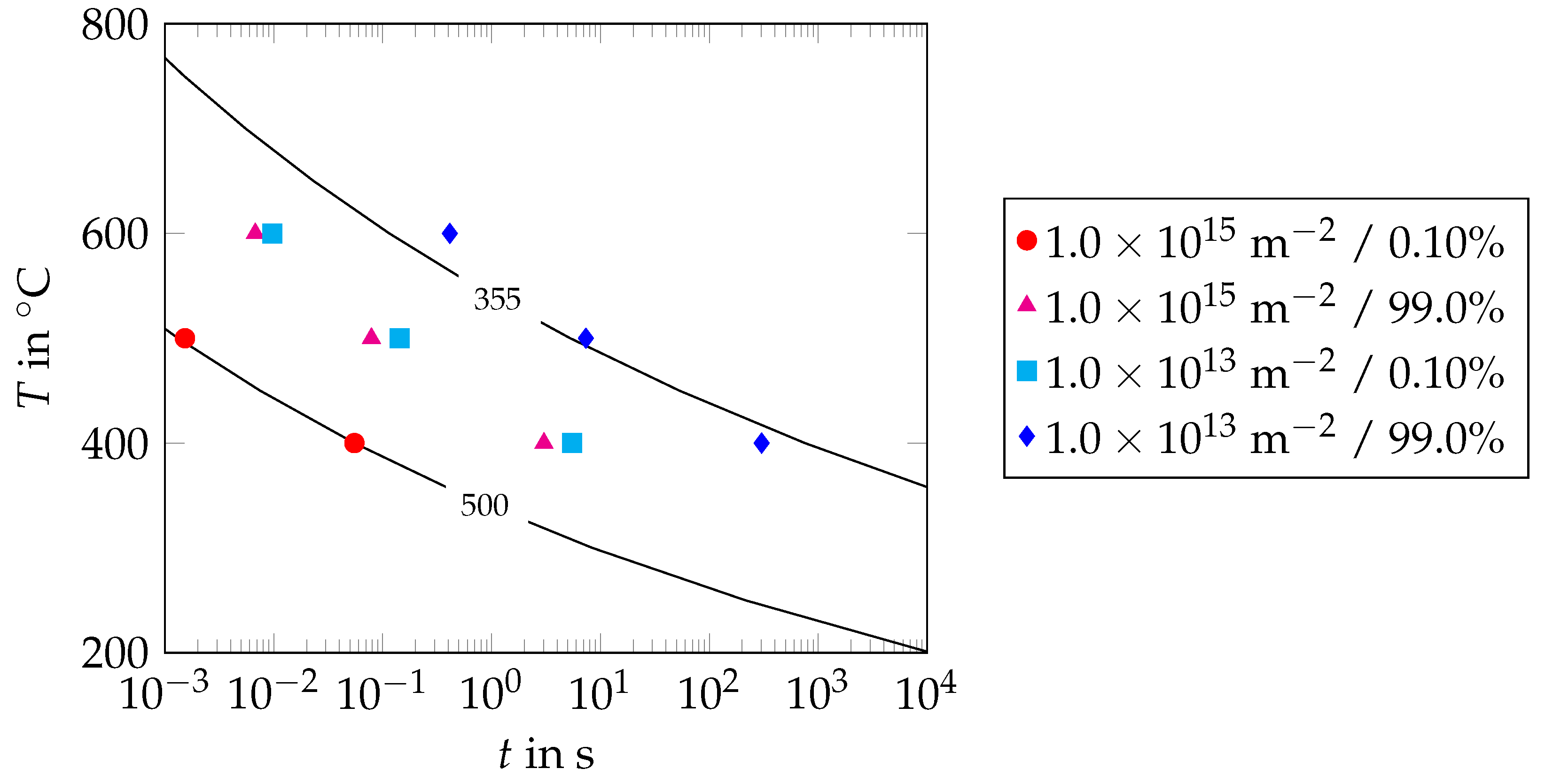
General Kinetics of Martensite Tempering
Kinetics of Cementite Precipitation
Change in the Specific Volume Due to Tempering
Changes in the Thermo-Mechanical Material Parameters
Transformation-Induced Plasticity
Modified Material Parameters
- To describe the theoretical volume change at 0 °C resulting from the transformation of austenite to martensite, Robl et al. [3] used a value of vol.%. The authors determined this value by carrying out a dilatometer measurement with a cylindrical specimen, which was made from the rebar steel grade B500B. In the dilatometer measurement, the specimen was quenched from austenitic state to room temperature with a cooling rate of 215 K/s. This cooling rate, however, was significantly lower than the cooling rates occurring during the partial quenching step of the TempCoreTM process. Due to this lower cooling rate and the high martensite start temperature of the rebar steel grade B500B, it seems likely that diffusion of carbon atoms to dislocations and grain boundaries already occurred during measurement. Both effects are associated with a negative volume change of approximately 0.15 vol.% (see also Section 4.1.2) and most likely do not occur in the partial quenching step during the TempCoreTM process. For this reason, the value of the theoretical volume change resulting from the transformation of austenite to martensite at 0 °C had to be corrected to a value of 3.09 vol.%.
- To describe the theoretical volume change resulting from the transformation of austenite into the mixture of bainite, pearlite and ferrite at 0 °C, Robl et al. [3] determined a value of vol.%. For the linear thermal expansion coefficient, the authors determined a value of 1/K. Both values were identified by carrying out dilatometer measurements with a cylindrical specimen, which was cooled down from austenitic state to room temperature with a cooling rate of approximately 3 K/s. Due to the low cooling rate, however, the specimen exhibited a ferritic–pearlitic microstructure after cooling. Therefore, the values determined by the authors, vol.% and 1/K, corresponded to the transformation of austenite into the mixture of ferrite and pearlite. Hence, the volume expansion due to the transformation of austenite into the mixture of bainite, pearlite and ferrite during the TempCoreTM process as well as the linear thermal expansion coefficient of this mixture, were captured only approximately in the model of Robl et al. [3]. An improved approximation of both parameter values is provided by the following approach. For low-alloyed steels, the theoretical volume change resulting from the transformation of austenite into bainite at 0 °C has been reported as approximately in the literature [55]. The linear thermal expansion coefficient has been reported as approximately [55]. Taking this into account, the theoretical volume change due to the transformation of austenite into the mixture of bainite, pearlite and ferrite, vol.%, and the linear thermal expansion coefficient of this mixture, 1/K, was approximated by using the linear rule of mixture. For this, the area fractions of bainite and of pearlite+ferrite in the cross-section of the rebar specimen estimated in Section 3.3 were taken into account.
4.1.3. Material Behavior of the Thin Surface Layer
4.2. Results and Discussion
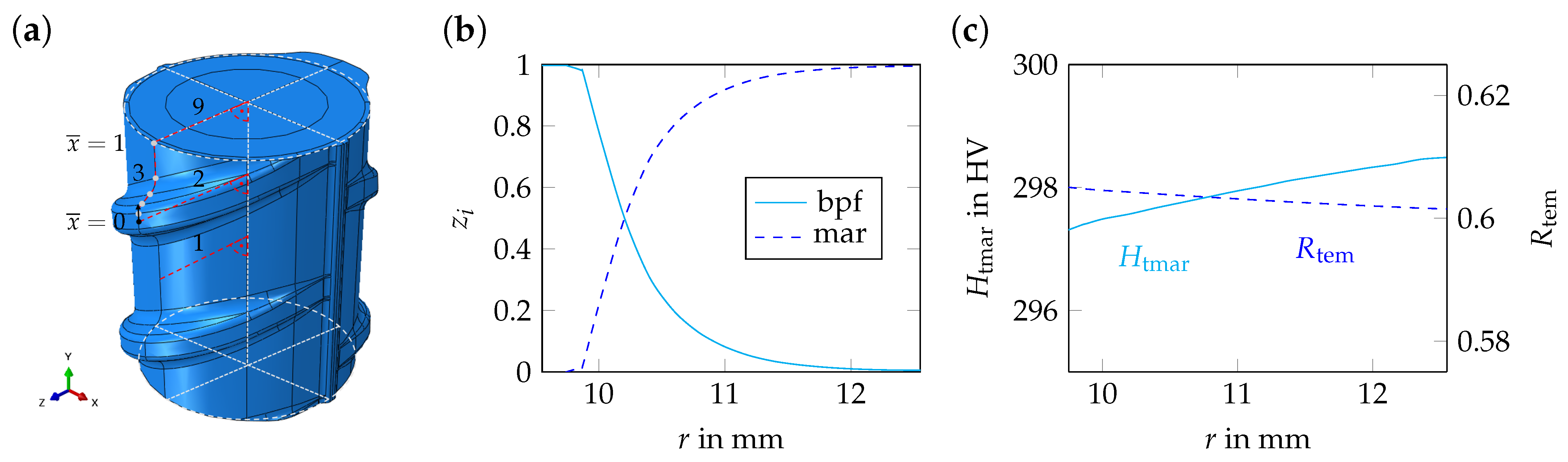
4.2.1. Phase Distribution and Mechanical Properties
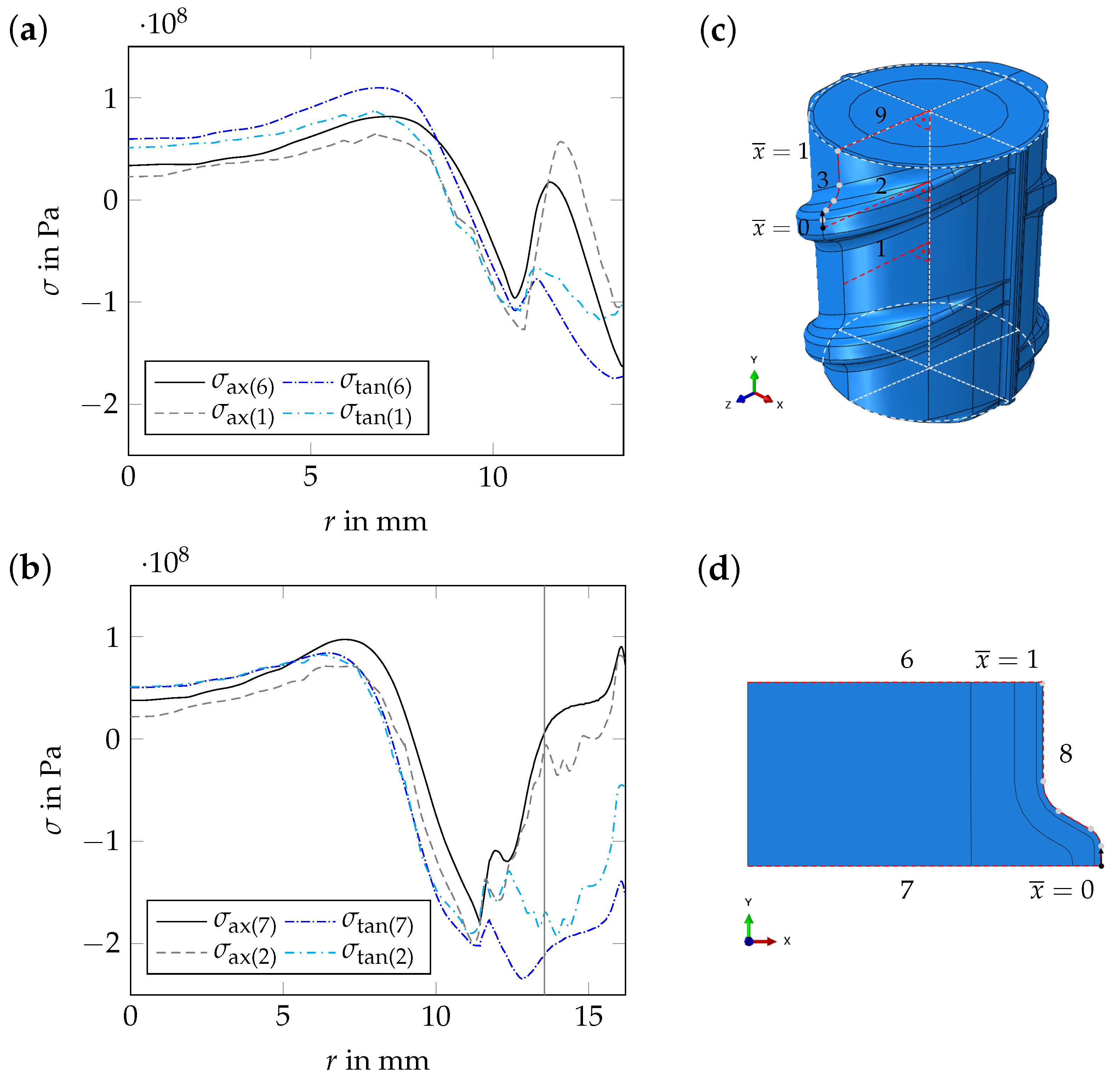
4.2.2. Residual Stress Distribution after Complete Cooling
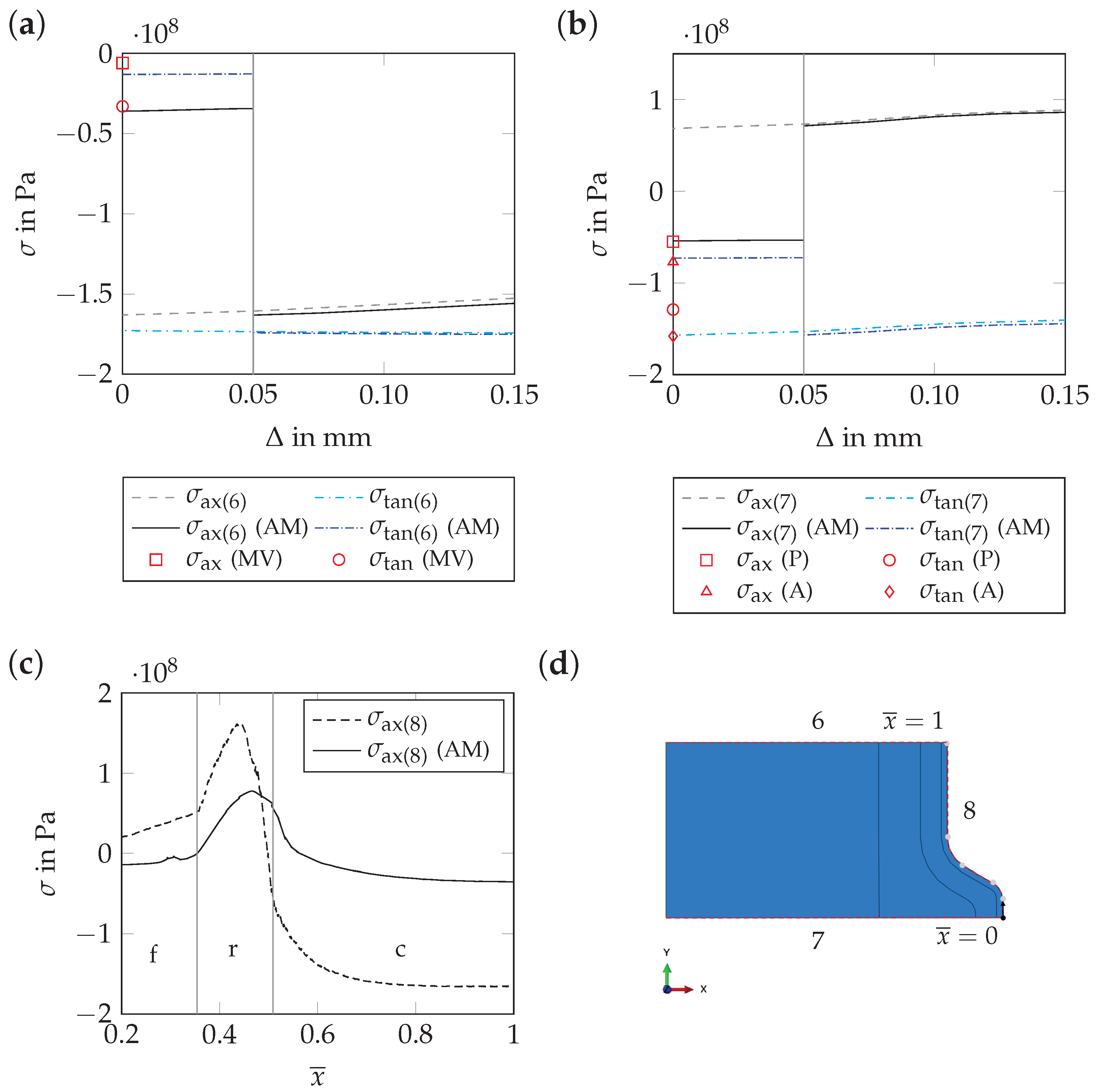
4.2.3. Effect of the Thin Surface Layer on Near-Surface Residual Stresses
4.2.4. Origin of the Residual Stresses
5. Summary
Author Contributions
Funding
Data Availability Statement
Conflicts of Interest
References
- DIN. DIN-488-2:2009-08; Reinforcing Steels—Reinforcing Steel Bars. Beuth: Berlin, Germany, 2009.
- DIN. DIN-488-1:2009-08; Reinforcing Steels—Part 1: Grades, Properties, Marking. Beuth: Berlin, Germany, 2009.
- Robl, T.; Wölfle, C.H.; Shahul Hameed, M.Z.; Rappl, S.; Krempaszky, C.; Werner, E. An approach to predict geometrically and thermo-mechanically induced stress concentrations in ribbed reinforcing bars. Metals 2022, 12, 411. [Google Scholar] [CrossRef]
- Economopoulos, M.; Respen, Y.; Lessel, G.; Steffes, G. Application of the tempcore process to the fabrication of high yield strength concrete-reinforcing bars. Metall. Rep. 1975, 45, 1–17. [Google Scholar]
- Noville, J.F. TEMPCORE, the most convenient process to produce low cost high strength rebars from 8 to 75 mm. In Proceedings of the METEC & 2nd ESTAD, Düsseldorf, Germany, 15–19 June 2015. [Google Scholar]
- Liscic, B.; Tensi, H.M.; Luty, W. Theory and Technology of Quenching; Springer: Berlin/Heidelberg, Germany, 1992. [Google Scholar]
- Volkwein, A.; Osterminski, K.; Meyer, F.; Gehlen, C. Distribution of residual stresses in reinforcing steel bars. Eng. Struct. 2020, 223, 111140. [Google Scholar] [CrossRef]
- Zheng, H.; Abel, A. Fatigue properties of reinforcing steel produced by TEMPCORE process. J. Mater. Civ. Eng. 1999, 11, 158–165. [Google Scholar] [CrossRef]
- Rocha, M.; Brühwiler, E.; Nussbaumer, A. Geometrical and material characterization of quenched and self-tempered steel reinforcement bars. J. Mater. Civ. Eng. 2016, 28, 04016012. [Google Scholar] [CrossRef]
- Zheng, H.; Abel, A. Stress concentration and fatigue of profiled reinforcing bars. Int. J. Fatigue 1998, 20, 767–773. [Google Scholar] [CrossRef]
- Hameed, M.Z.; Wölfle, C.H.; Robl, T.; Obermayer, T.; Rappl, S.; Osterminski, K.; Krempaszky, C.; Werner, E. Parameter identification for thermo-mechanical constitutive modeling to describe process-induced residual stresses and phase transformations in low-carbon steels. Appl. Sci. 2021, 11, 550. [Google Scholar] [CrossRef]
- Bhadeshia, H.; Honeycombe, R. Steels: Microstructure and Properties; Butterworth-Heinemann: Oxford, UK, 2017. [Google Scholar]
- Speich, G.R.; Leslie, W.C. Tempering of steel. Metall. Trans. 1972, 3, 1043–1054. [Google Scholar] [CrossRef]
- Fischer, F.D.; Sun, Q.-P.; Tanaka, K. Transformation–induced plasticity (TRIP). Appl. Mech. Rev. 1996, 49, 317–364. [Google Scholar] [CrossRef]
- Fischer, F.D.; Reisner, G.; Werner, E.; Tanaka, K.; Cailletaud, G.; Antretter, T.A. New view on transformation induced plasticity (TRIP). Int. J. Plast. 2000, 16, 723–748. [Google Scholar] [CrossRef]
- Greenwood, G.W.; Johnson, R.H. The deformation of metals under small stresses during phase transformation. Proc. Roy. Soc. 1965, 283, 403–422. [Google Scholar]
- Wölfle, C.H. Numerische Untersuchung einer Kontinuumsformulierung für die Thermoelastoplastizität von Stählen unter Phasenumwandlungen. Masters’s Thesis, Technical University of Munich, Munich, Germany, 2018. [Google Scholar]
- Magee, C.L. Transformation Kinetics, Micro-Plasticity and Aging of Martensite in Fe–31 Ni. Ph.D. Thesis, Carnegie Institute of Technology, Pittsburgh, PA, USA, 1966. [Google Scholar]
- Wechsler, M.S.; Liebermann, D.S.; Read, T.A. On the theory of the formation of martensite. Trans. Am. Inst. Min. Metall. Eng. 1953, 197, 1503–1515. [Google Scholar]
- Patel, J.R.; Cohen, M. Criterion for the action of applied stress in the martensitic transformation. Acta. Metall. 1953, 1, 531–538. [Google Scholar] [CrossRef]
- Rappl, S.; Shahul Hameed, M.Z.; Krempaszky, C.; Osterminski, K. Mechanical and surface geometric properties of reinforcing bars and their significance for the development of near-surface notch stresses. Mathematics 2023, 11, 1910. [Google Scholar] [CrossRef]
- He, B.B. Two-Dimensional X-ray Diffraction; Wiley Online Library: Hoboken, NJ, USA, 2009. [Google Scholar]
- Hofle, M.; Roth, A.; Hegele, P.; Schubert, T.; Schanz, J.; Harrison, D.K.; De Silva, A.K.M.; Riegel, H. Influence of laser polishing on the material properties of aluminium L-PBF components. Metals 2022, 12, 750. [Google Scholar] [CrossRef]
- Niessen, F.; Nyyssönen, T.; Gazder, A.A.; Hielscher, R. Parent grain reconstruction from partially or fully transformed microstructures in MTEX. J. Appl. Cryst. 2022, 55, 180–194. [Google Scholar] [CrossRef]
- Hielscher, R.; Nyyssönen, T.; Niessen, F.; Gazder, A.A. The variant graph approach to improved parent grain reconstruction. Mater. 2022, 22, 101399. [Google Scholar] [CrossRef]
- Bachmann, F.; Hielscher, R.; Schaeben, H. Texture analysis with MTEX—Free and open source software toolbox. Solid State Phenom. 2010, 160, 63–68. [Google Scholar] [CrossRef]
- Smith, M. ABAQUS/Standard User’s Manual; Dassault Systemes Simulia Corp.: Johnston, FI, USA, 2014. [Google Scholar]
- Dassault Systemes Solid Works Corp. Solid Works; Solid Works Corp.: Waltham, MA, USA, 2019. [Google Scholar]
- Bandyopadhyay, K.; Lee, J.; Shim, J.-H.; Hwang, B.; Lee, M.-G. Modeling and experiment on microstructure evolutions and mechanical properties in grade 600 MPa reinforcing steel rebar subjected to TempCore process. Mater. Sci. Eng. A 2019, 745, 39–52. [Google Scholar] [CrossRef]
- Lippmann, H. Mechanik des Plastischen Fließens; Springer: Berlin/Heidelberg, Germany, 1981. [Google Scholar]
- Koistinen, D.P.; Marburger, R.E. A general equation prescribing the extent of the austenite-martensite transformation in pure iron-carbon alloys and plain carbon steels. Acta. Metall. 1959, 7, 59–60. [Google Scholar] [CrossRef]
- Kolmogorov, A.N. On the statistical theory of the crystallization of metals. Bull. Acad. Sci. USSR Math. Ser. 1937, 1, 355–359. [Google Scholar]
- Johnson, W.A.; Mehl, R.F. Reaction kinetics in processes of nucleation and growth. Trans. Am. Inst. Min. Metall. Eng. 1939, 135, 416–442. [Google Scholar]
- Avrami, M. Kinetics of phase change. I General theory. J. Chem. Phys. 1939, 7, 1103–1112. [Google Scholar] [CrossRef]
- Avrami, M. Kinetics of phase change. II Transformation-time relations for random distribution of nuclei. J. Chem. Phys. 1940, 8, 212–224. [Google Scholar] [CrossRef]
- Sun, Y.L.; Obasi, G.; Hamelin, C.J.; Vasileiou, A.N.; Flint, T.F.; Francis, J.A.; Smith, M.C. Characterisation and modeling of tempering during multi-pass welding. J. Mater. Process. Technol. 2019, 270, 118–131. [Google Scholar] [CrossRef]
- Kang, S.; Lee, S.-J. Prediction of tempered martensite hardness incorporating the composition-dependent tempering parameter in low alloy steels. Mater. Trans. 2014, 55, 1069–1072. [Google Scholar] [CrossRef]
- Grange, R.A.; Hribal, C.R.; Porter, L.F. Hardness of tempered martensite in carbon and low-alloy steels. Metall. Mater. Trans. A 1977, 8, 1775–1785. [Google Scholar] [CrossRef]
- MatCalc Engineering GmbH. MatCalc 6; MatCalc Engineering GmbH: Vienna, Austria, 2022. [Google Scholar]
- Zamberger, S.; Whitmore, L.; Krisam, S.; Wojcik, T.; Kozeschnik, E. Experimental and computational study of cementite precipitation in tempered martensite. Model. Simul. Mat. Sci. Eng. 2015, 23, 055012. [Google Scholar] [CrossRef]
- Morito, S.; Nishikawa, J.; Maki, T. Dislocation density within lath martensite in Fe-C and Fe-Ni alloys. ISIJ Int. 2003, 9, 1475–1477. [Google Scholar] [CrossRef]
- Cheng, L.; Van der Pers, N.M.; Böttger, A.; Keijser, T.H. Lattice changes of iron–carbon martensite on aging at room temperature. Metall. Trans. A 1991, 22A, 1957–1967. [Google Scholar] [CrossRef]
- Waterschoot, T.; Verbeken, K.; De Coman, B.C. Tempering kinetics of the martensitic phase in DP steel. ISIJ Int. 2006, 46, 138–146. [Google Scholar] [CrossRef]
- Kagawa, A.; Okamoto, T.; Matsumoto, H. Young’s modulus and thermal expansion of pure iron-cementite alloy castings. Acta. Metall. 1987, 35, 797–803. [Google Scholar] [CrossRef]
- DIN-50150:1976-12; Umwertungstabelle für Vickershärte, Brinellhärte, Rockwellhärte und Zugfestigkeit. Beuth: Berlin, Germany, 1976.
- Säglitz, M.; Matlock, D.K.; Kraus, G. Tempering and mechanical properties of low-carbon boron-containing martensitic sheet steel. In Proceedings of the International Conference on New Developments in Advanced High-Strength Sheet Steels, Warrendale, PA, USA, 15–18 June 2008. [Google Scholar]
- Otsuka, T.; Akashi, T.; Ogawa, S.; Imai, T.; Egami, A. Effect of volume expansion on transformation plasticity during ferrite and martensite transformation in steel. J. Soc. Mater. Sci. Jpn. 2011, 60, 937–942. [Google Scholar] [CrossRef]
- Giusti, J. Contraintes et Déformations Résiduelles d’Origine Thermique. Application au Soudage et à la Trempe des Aciers. Ph.D. Thesis, University Pierre et Marie Curie, Paris, France, 1981. [Google Scholar]
- Jiang, W.; Chen, W.; Woo, W.; Tu, S.-T.; Zhang, X.-C.; Em, V. Effects of low-temperature transformation and transformation-induced plasticity on weld residual stresses: Numerical study and neutron diffraction measurement. Mater. Des. 2018, 147, 65–79. [Google Scholar] [CrossRef]
- Deng, D.; Murakawa, H. Influence of transformation induced plasticity on simulated results of welding residual stress in low temperature transformation steel. Comput. Mat. Sci. 2013, 78, 55–62. [Google Scholar] [CrossRef]
- Miyao, K.; Wang, Z.-G.; Inoue, T. Analysis of temperature, stress and metallic structure in carburized-quenched gear considering transformation plasticity. J. Soc. Mater. Sci. Jpn. 1986, 35, 1352–1357. [Google Scholar] [CrossRef]
- Nagasaka, Y.; Brimacombe, J.K.; Hawbolt, E.B.; Samarasekera, I.V.; Hernandez-Morales, B.; Chidiac, S.E. Mathematical model of phase transformations and elasto-plastic stress in the water spray quenching of steel bars. Metall. Mater. Trans. A 1993, 24, 795–808. [Google Scholar] [CrossRef]
- Mitter, W. Umwandlungsplastizität und ihre Berücksichtigung bei der Berechnung von Eigenspannungen; Gebrüder Borntraeger: Berlin-Stuttgart, Germany, 1987. [Google Scholar]
- Eres-Castellanos, A.; Toda-Caraballo, I.; Latz, A.; Caballero, F.G.; Garcia-Mateo, C. An integrated-model for austenite yield strength considering the influence of temperature and strain rate in lean steels. Mater. Des. 2020, 188, 108435. [Google Scholar] [CrossRef]
- Ariza, E.A.; Martorano, M.A.; de Lima, N.B.; Tschiptschin, A.P. Numerical simulation with thorough experimental validation to predict the build-up of residual stresses during quenching of carbon and low-alloy steels. ISIJ Int. 2014, 54, 1396–1405. [Google Scholar] [CrossRef]
- Liu, C.; Zhao, Z.; Northwood, D.O.; Liu, Y. A new empirical formula for the calculation of MS temperatures in pure iron and super–low carbon alloy steels. J. Mater. Process. Technol. 2001, 113, 556–562. [Google Scholar] [CrossRef]


| Stress Component | Symbol | A | B | C | D | E | F | G | H | I | J |
|---|---|---|---|---|---|---|---|---|---|---|---|
| Axial stress component | −2 | −11 | −8 | −1 | −22 | −77 | −9 | −55 | 7 | 0 | |
| Tangential stress component | −24 | −41 | −15 | −36 | −44 | −158 | −49 | −129 | −34 | −20 |
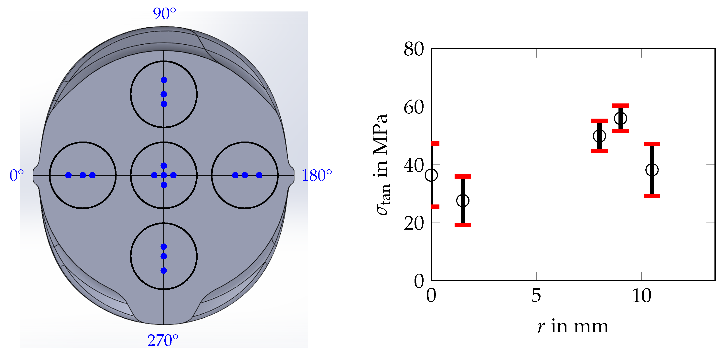
| r in mm | 0° | 90° | 180° | 270° | MV | STD |
|---|---|---|---|---|---|---|
| 0.0 | 46.0 | 32.9 | 46.7 | 20.2 | 35.5 | 10.9 |
| 1.5 | 36.0 | 19.3 | (−27.4) | (10.6) | 27.7 | 8.4 |
| 8.0 | (−35.8) | 44.8 | 47.9 | 57.1 | 49.9 | 5.2 |
| 9.0 | (8.2) | 60.4 | (67.9) | 51.6 | 56.0 | 4.4 |
| 10.5 | 50.5 | (46.9) | 29.3 | 35.0 | 38.3 | 9.0 |
| Rebar | Symbol | Reference Value | Unit |
|---|---|---|---|
| Rebar diameter (1) | d | 28.00 | mm |
| Bar diameter (2) | 27.10 | mm | |
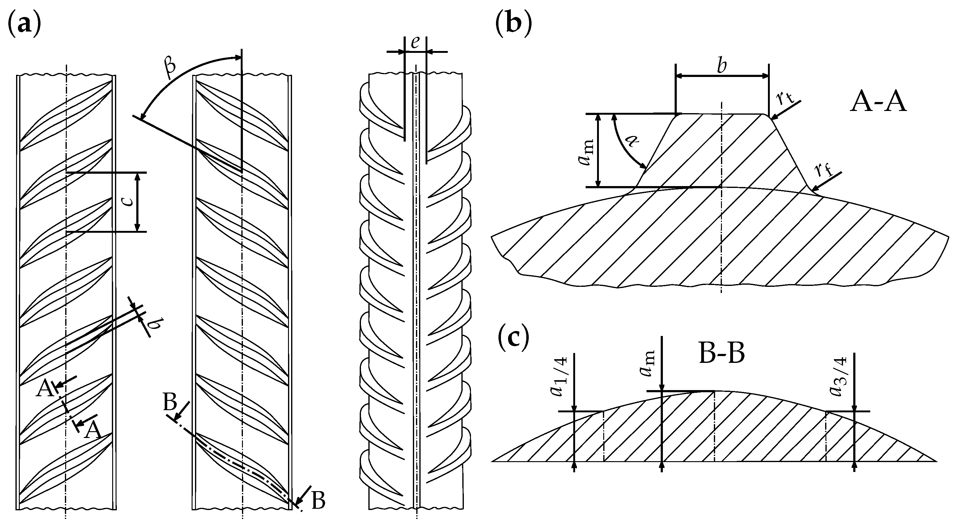
| Transverse Ribs | Symbol | Reference Value | Unit |
| Distance between rib rows | e | 2.00 | mm |
| Rib spacing | c | 16.80 | mm |
| Foot radius | 1.60 | mm | |
| Tip radius | 0.84 | mm | |
| Rib width | b | 2.80 | mm |
| Rib heigth (middle of the rib) | 2.60 | mm | |
| Rib heigth (one-/three-quarter point) | , | 1.80 | mm |
| Flank inclination | 65 | ||
| Rib inclination | 60 | ||
| Longitudinal Ribs | Symbol | Reference Value | Unit |
| Foot radius | 1.00 | mm | |
| Tip radius | 0.60 | mm | |
| Rib width | 2.00 | mm | |
| Rib heigth | 0.60 | mm | |
| Flank inclination | 90 |
| [C] | [C] | [s] | [s] | [W/m2K] | [W/m2K] |
|---|---|---|---|---|---|
| 950 (1) | 20 (2) | 1.5 (3) | 2998.5 (4) | 34,000 (3) | 40 (1) |
| T [] | [MPa] | [MPa] |
|---|---|---|
| 0 | 1315 | 530 |
| 200 | 1065 | 420 (1) |
| 300 | 395 | 388 (1) |
| 600 | 118 | 116 (1) |
Disclaimer/Publisher’s Note: The statements, opinions and data contained in all publications are solely those of the individual author(s) and contributor(s) and not of MDPI and/or the editor(s). MDPI and/or the editor(s) disclaim responsibility for any injury to people or property resulting from any ideas, methods, instructions or products referred to in the content. |
© 2023 by the authors. Licensee MDPI, Basel, Switzerland. This article is an open access article distributed under the terms and conditions of the Creative Commons Attribution (CC BY) license (https://creativecommons.org/licenses/by/4.0/).
Share and Cite
Robl, T.; Hegele, P.; Krempaszky, C.; Werner, E. Residual Stresses in Ribbed Reinforcing Bars. Materials 2024, 17, 26. https://doi.org/10.3390/ma17010026
Robl T, Hegele P, Krempaszky C, Werner E. Residual Stresses in Ribbed Reinforcing Bars. Materials. 2024; 17(1):26. https://doi.org/10.3390/ma17010026
Chicago/Turabian StyleRobl, Tobias, Patrick Hegele, Christian Krempaszky, and Ewald Werner. 2024. "Residual Stresses in Ribbed Reinforcing Bars" Materials 17, no. 1: 26. https://doi.org/10.3390/ma17010026
APA StyleRobl, T., Hegele, P., Krempaszky, C., & Werner, E. (2024). Residual Stresses in Ribbed Reinforcing Bars. Materials, 17(1), 26. https://doi.org/10.3390/ma17010026