
Optimizing the Utilization of Steel Slag in Cement-Stabilized Base Layers: Insights from Freeze–Thaw and Fatigue Testing


Abstract
:1. Introduction
2. Experimental Procedures
2.1. Materials
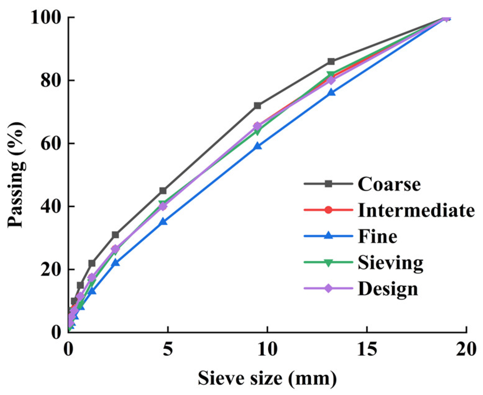
2.2. Design of Mix Ratio for CSS
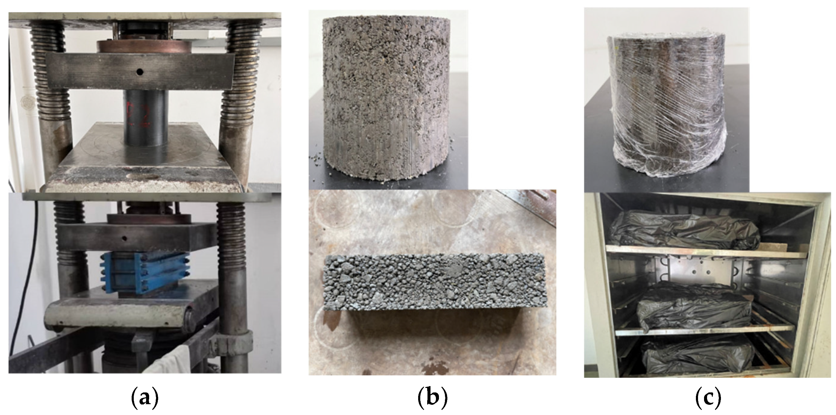
2.3. Specimen Preparation
2.4. Unconfined Compressive Strength Test
2.5. Freeze–Thaw Cycle Test
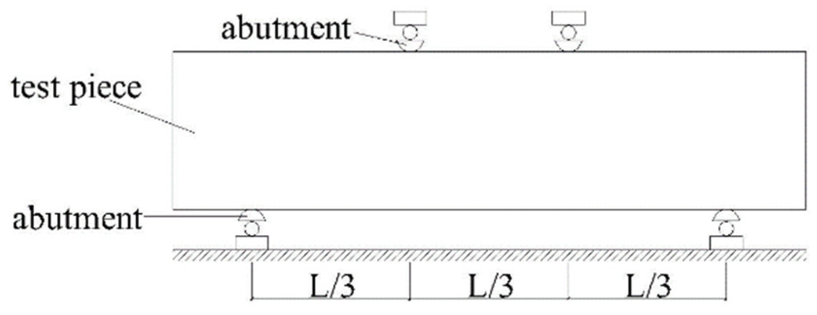
2.6. Bending Strength Test and Fatigue Test
3. Construction of Discrete Element Numerical Simulation Model Based on 3D Scanning Technology
3.1. 3D Scanning of Steel Slag Stones
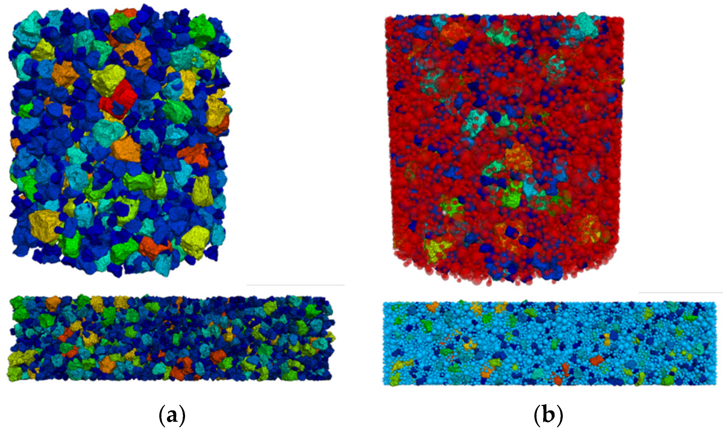
3.2. Construction of Stochastic Discrete Element Models Based on 3D Scanning
3.3. Sensitivity Analyses between Macro- and Fine-Scale Parameters
3.3.1. Selection of Orthogonal Test Macro- and Fine-Scale Parameters
3.3.2. Orthogonal Test Design Scheme and Calculation Results
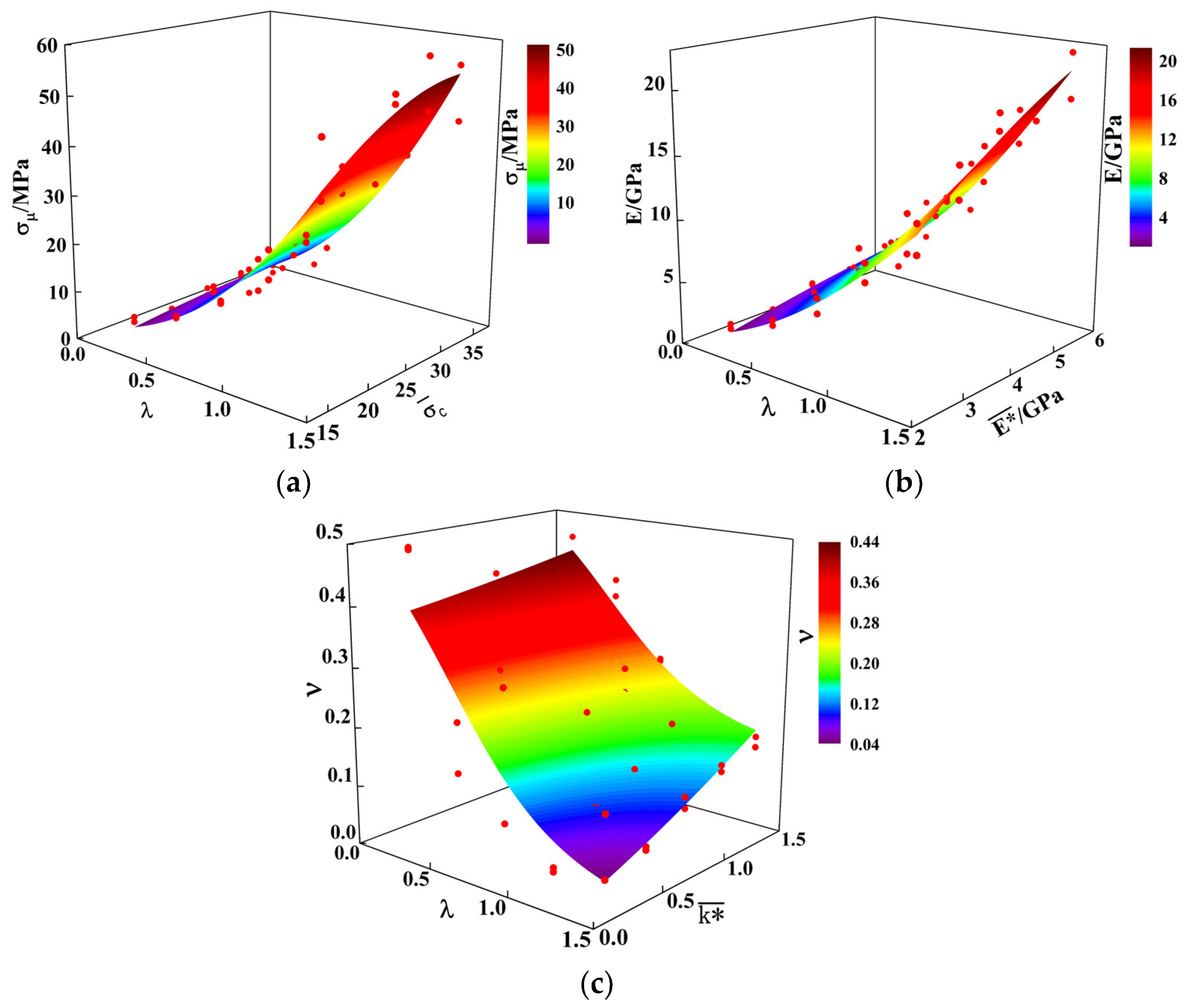
3.3.3. Sensitivity Analyses between Macro- and Fine-Scale Parameters
3.4. Calibration of Discrete Element Parameters for CSS
4. Discrete Element Numerical Simulation Study of CSS
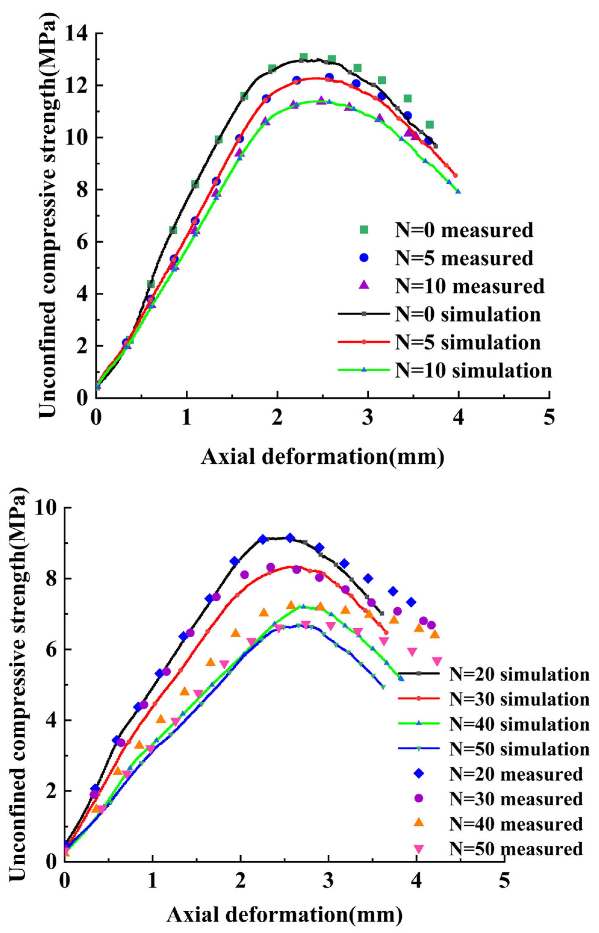
4.1. Uniaxial Compression Discrete Element Simulation of Freeze–Thaw Damaged CSS
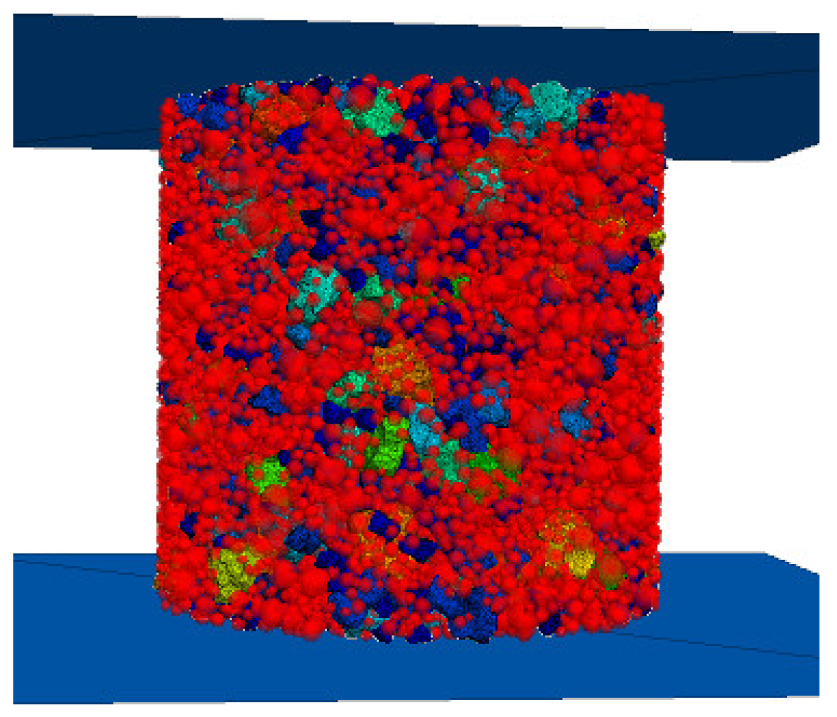
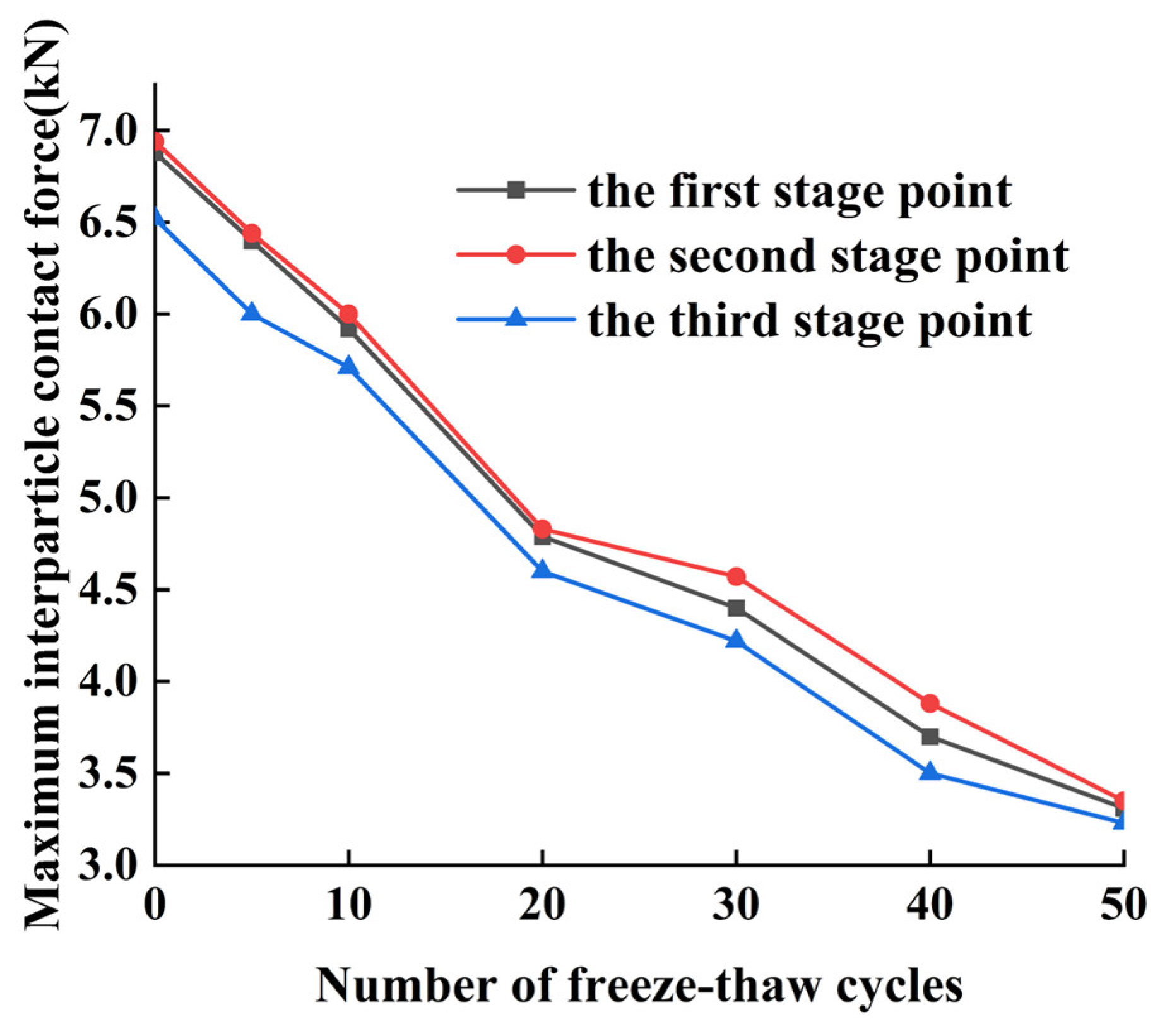
4.1.1. Analysis of Contact Forces between Particles of CSS
4.1.2. Crack Development Pattern of CSS Model
4.2. Numerical Simulation of Frost–Thaw-Damaged CSS Mixes in Flexural and Fatigue Tests
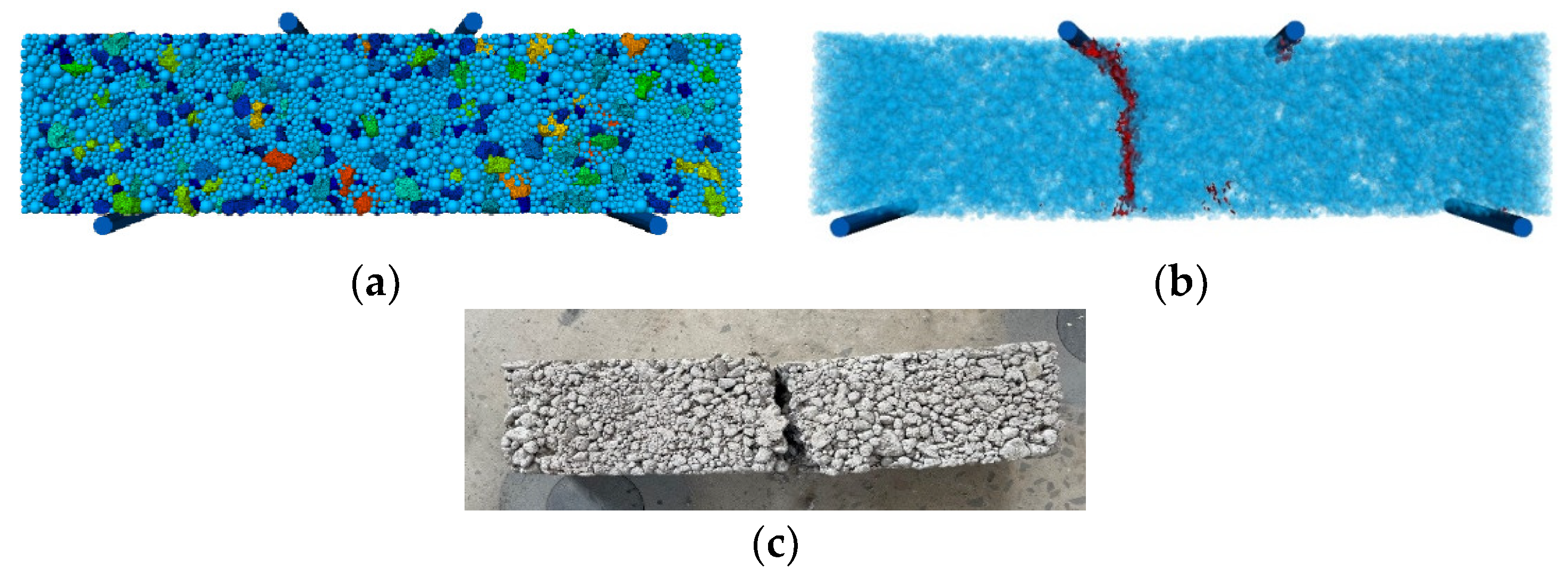
4.2.1. Bending Simulation Tests on Beam Specimens of CSS Mixes
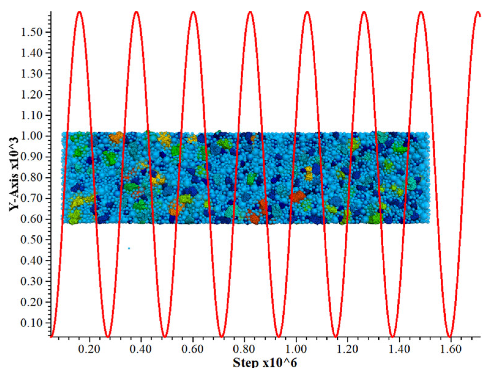
4.2.2. Effect of Freeze–Thaw Cycles on Fatigue Life of CSS Mixes
4.3. Damage Modeling of CSS under Coupled Load–Freeze–Thaw Cycles
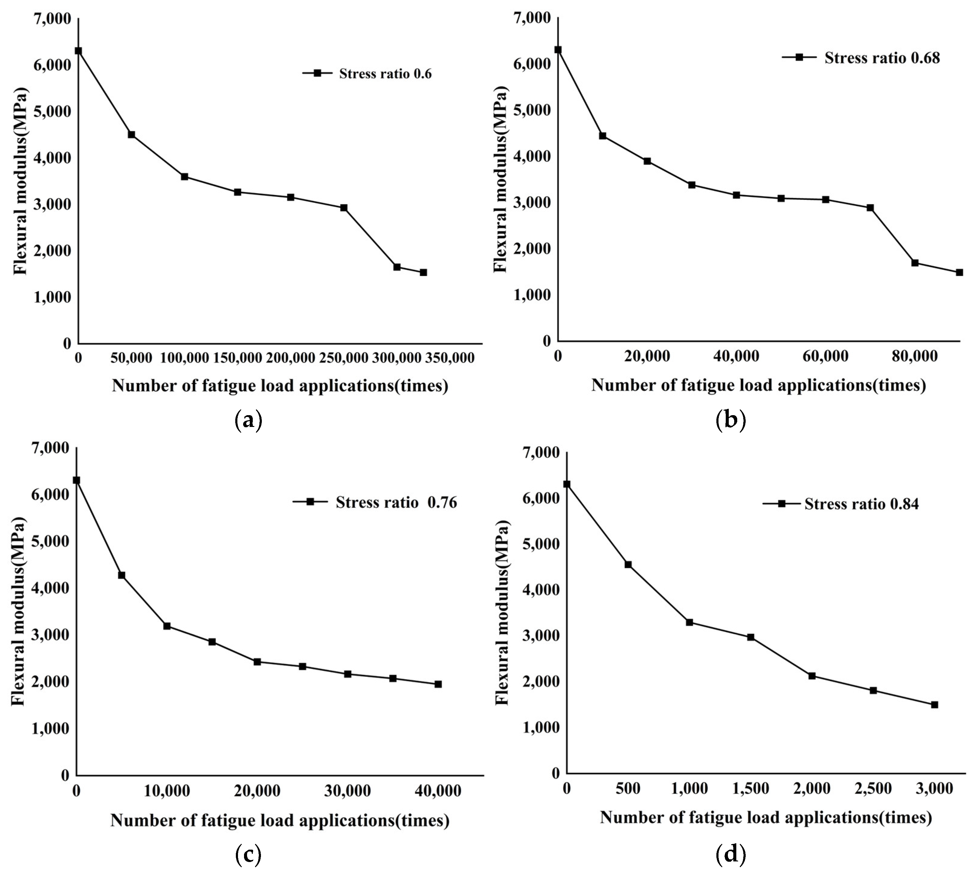
4.3.1. Flexural Strength Decay Law of Materials under the Effect of Fatigue Damage
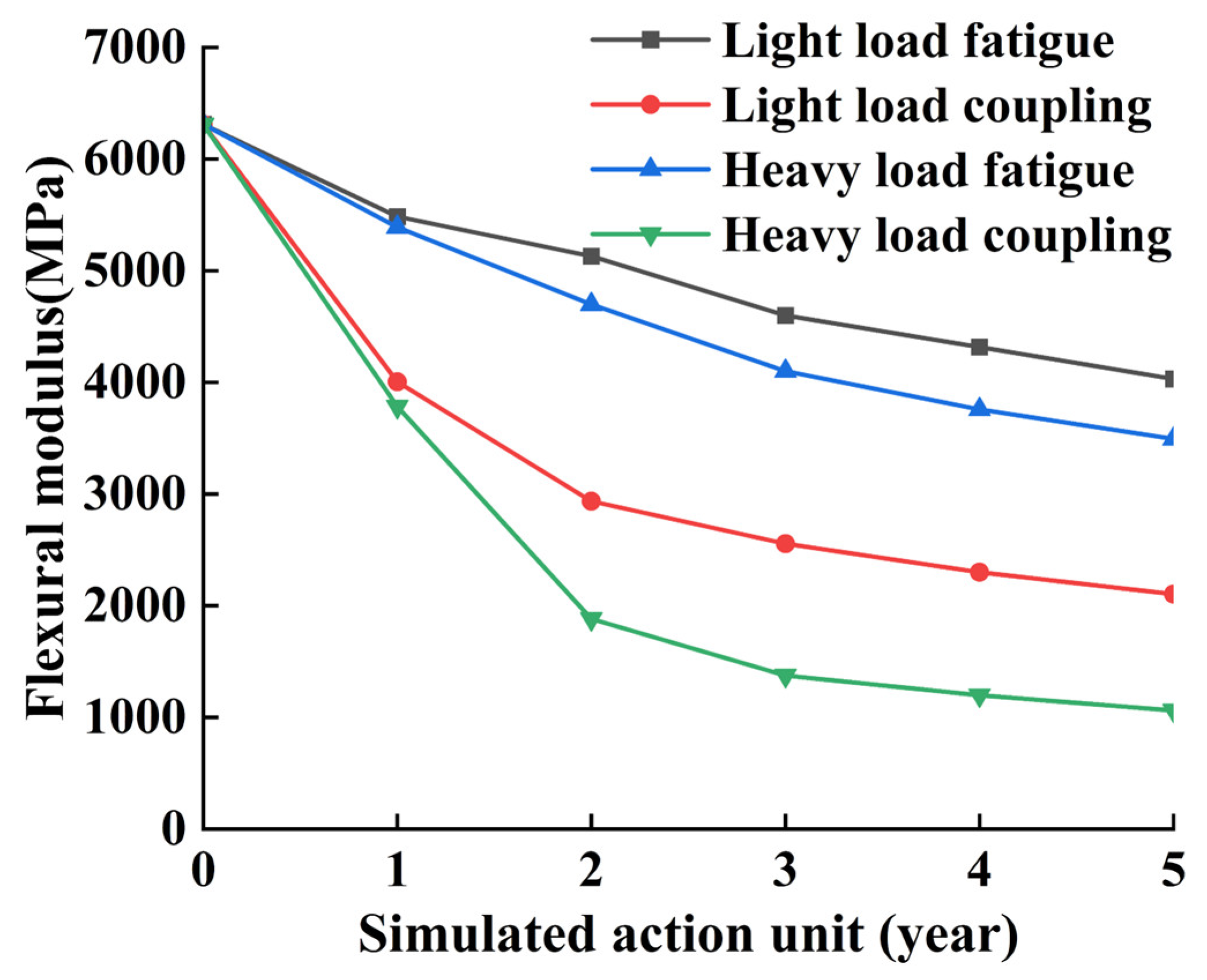
4.3.2. Bending Modulus Decay Law under Fatigue Loading–Freeze–Thaw Cycle Coupled Damage
5. Conclusions
- (1)
- The best cement dosage of the specimen is 5%; although 4.5%, 5%, and 5.5% are three kinds of cement dosage that can meet the specification of the extra heavy traffic state of the pavement grass-roots bearing capacity requirements, the cement dosage of 4.5% results in a specimen with an overall looseness of surface roughness, with the fine aggregates falling off; and cement dosage of 5.5% results in a specimen which, after 7 days of the curing period, due to the expansion of ettringite in the excess cement and the micro-expansion of the steel slag, had cracks appeared on a small part of its surface. The specimen with 5% of cement mixing had a better integrity and no obvious defects.
- (2)
- Using three-dimensional scanning technology and orthogonal experimental design to analyze the sensitivity relationship between the parameters in the discrete element software, we obtained that has a significant effect on , , and , and that , , and have a significant effect on , , and , respectively, and we fitted the non-linear relationship equation between the parameters; after the uniaxial compression simulation, the obtained stress–strain curves have a high degree of restoration in comparison with the laboratory-measured curves, which indicates the correctness of the calibration parameters. The maximum value of the contact force and the main cracks are distributed in the shear zone region of the specimen, and the number of shear cracks throughout the compression damage is more than the number of tension cracks, so the compression damage is essentially a mixed tensile–shear damage with shear damage as the main damage.
- (3)
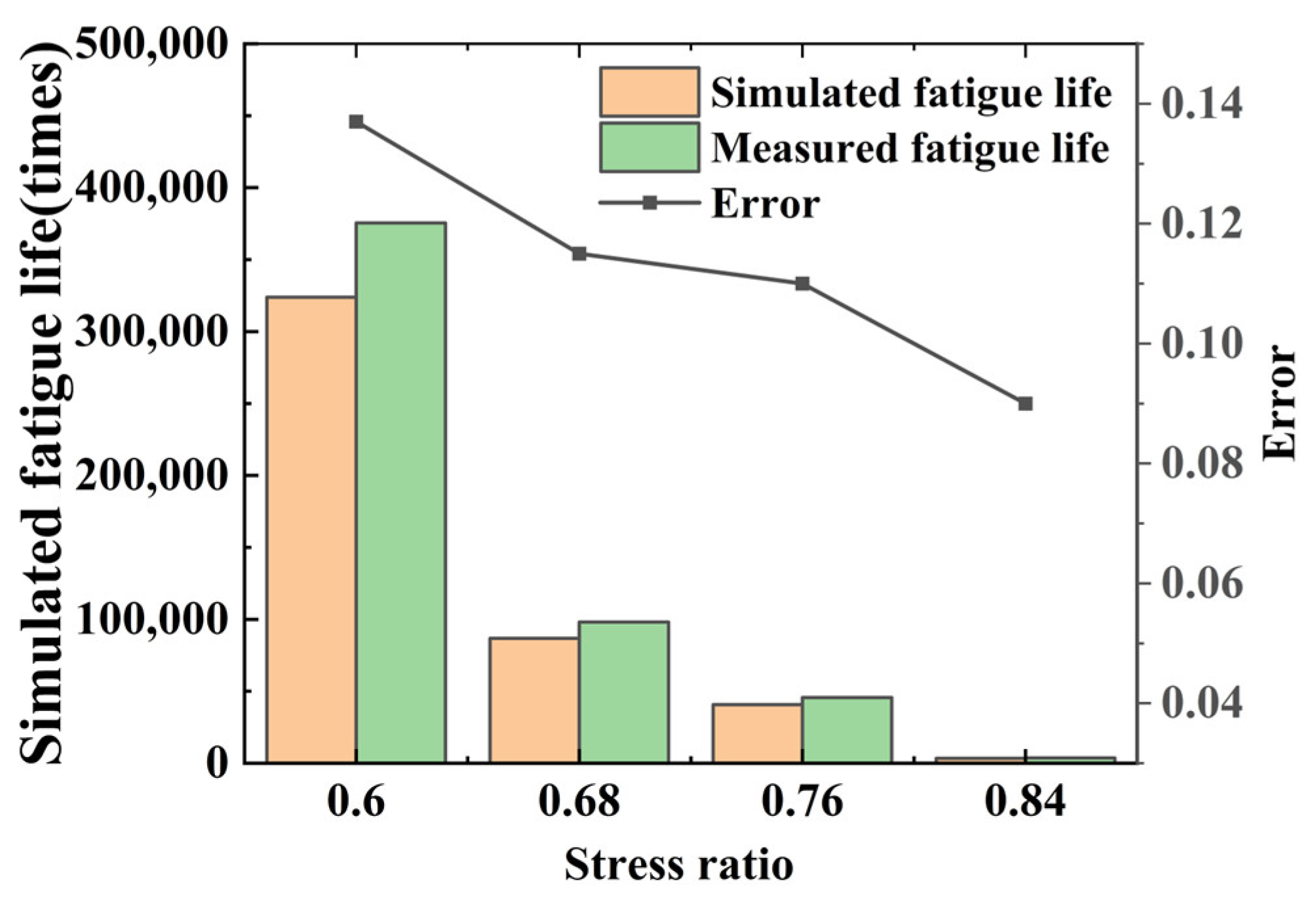
- In the bending strength experiment, the error between the measured laboratory breaking load and the breaking load obtained from the simulation test is only 1.24%. The error between the results of the fatigue test and the simulation is 8–14%, which decreases when the level of load acting on the specimen is increased. The specimen bending modulus under the action of fatigue loading at relatively low stress has three stages of change: a rapid decline period, a relatively smooth period, and a sudden change fracture period. When stress ratio is small, there is a critical value of change; when the stress ratio increases the decline phase is reduced, and the sudden change fracture period disappeared; in the freezing and thawing cycle–fatigue loading coupling, the first two years of the bending and tensile modulus drastically decreased to the original 50% or so, and with 3–5 years of the bending and tensile modulus, the decline tends to level off.
- (4)
- The next step could be to continue the study in the following two parts: research on the mechanical properties of specimens with different grades and cement contents subjected to freeze–thaw cycles; and research on the effect of multi-factor coupling (e.g., temperature–wet/dry-fatigue coupling) on the mechanical properties of cement-stabilized steel slag base layers.
Author Contributions
Funding
Institutional Review Board Statement
Informed Consent Statement
Data Availability Statement
Conflicts of Interest
References
- Wang, Z.; Sohn, I. A review on reclamation and reutilization of ironmaking and steelmaking slags. J. Sustain. Metall. 2019, 5, 127–140. [Google Scholar] [CrossRef]
- Semykina, A.; Shatokha, V.; Seetharaman, S. Innovative approach to recovery of iron from steelmaking slags. Ironmak. Steelmak. 2010, 37, 536–540. [Google Scholar] [CrossRef]
- Gao, X.; Okubo, M.; Maruoka, N.; Shibata, H.; Ito, T.; Kitamura, S.-Y. Production and utilisation of iron and steelmaking slag in Japan and the application of steelmaking slag for the recovery of paddy fields damaged by Tsunami. Miner. Process. Extr. Metall. 2015, 124, 116–124. [Google Scholar] [CrossRef]
- Cao, L.; Shen, W.; Huang, J.; Yang, Y.; Zhang, D.; Huang, X.; Lv, Z.; Ji, X. Process to utilize crushed steel slag in cement industry directly: Multi-phased clinker sintering technology. J. Clean. Prod. 2019, 217, 520–529. [Google Scholar] [CrossRef]
- Nidheesh, P.V.; Kumar, M.S. An overview of environmental sustainability in cement and steel production. J. Clean. Prod. 2019, 231, 856–871. [Google Scholar] [CrossRef]
- Guo, J.; Bao, Y.; Wang, M. Steel slag in China: Treatment, recycling, and management. Waste Manag. 2018, 78, 318–330. [Google Scholar] [CrossRef] [PubMed]
- Wang, X.; Li, X.; Yan, X.; Tu, C.; Yu, Z. Environmental risks for application of iron and steel slags in soils in China: A review. Pedosphere 2021, 31, 28–42. [Google Scholar] [CrossRef]
- Xue, Y.; Wu, S.; Hou, H.; Zha, J. Experimental investigation of basic oxygen furnace slag used as aggregate in asphalt mixture. J. Hazard. Mater. 2006, 138, 261–268. [Google Scholar] [CrossRef] [PubMed]
- Pasetto, M.; Baliello, A.; Giacomello, G.; Pasquini, E. Sustainable solutions for road pavements: A multi-scale characterization of warm mix asphalts containing steel slags. J. Clean. Prod. 2017, 166, 835–843. [Google Scholar] [CrossRef]
- Pasetto, M.; Baldo, N. Experimental evaluation of high performance base course and road base asphalt concrete with electric arc furnace steel slags. J. Hazard. Mater. 2010, 181, 938–948. [Google Scholar] [CrossRef]
- Skaf, M.; Manso, J.M.; Aragón, Á.; Fuente-Alonso, J.A.; Ortega-López, V. EAF slag in asphalt mixes: A brief review of its possible re-use. Resour. Conserv. Recycl. 2017, 120, 176–185. [Google Scholar] [CrossRef]
- Chen, J.S.; Wei, S.H. Engineering properties and performance of asphalt mixtures incorporating steel slag. Constr. Build. Mater. 2016, 128, 148–153. [Google Scholar] [CrossRef]
- Pasetto, M.; Baliello, A.; Giacomello, G.; Pasquini, E. Rheological characterization of warm-modified asphalt mastics containing electric arc furnace steel slags. Adv. Mater. Sci. Eng. 2016, 2016, 9535940. [Google Scholar] [CrossRef]
- Alinezhad, M.; Sahaf, A. Investigation of the fatigue characteristics of warm stone matrix asphalt (WSMA) containing electric arc furnace (EAF) steel slag as coarse aggregate and Sasobit as warm mix additive. Case Stud. Constr. Mater. 2019, 11, e00265. [Google Scholar] [CrossRef]
- Wu, S.; Xue, Y.; Ye, Q.; Chen, Y. Utilization of steel slag as aggregates for stone mastic asphalt (SMA) mixtures. Build. Environ. 2007, 42, 2580–2585. [Google Scholar] [CrossRef]
- Goli, H.; Hesami, S.; Ameri, M. Laboratory evaluation of damage behavior of warm mix asphalt containing steel slag aggregates. J. Mater. Civ. Eng. 2017, 29, 04017009. [Google Scholar] [CrossRef]
- Gao, J.; Sha, A.; Wang, Z.; Tong, Z.; Liu, Z. Utilization of steel slag as aggregate in asphalt mixtures for microwave deicing. J. Clean. Prod. 2017, 152, 429–442. [Google Scholar] [CrossRef]
- Sun, Y.; Wu, S.; Liu, Q.; Zeng, W.; Chen, Z.; Ye, Q.; Pan, P. Self-healing performance of asphalt mixtures through heating fibers or aggregate. Constr. Build. Mater. 2017, 150, 673–680. [Google Scholar] [CrossRef]
- Phan, T.M.; Park, D.W.; Le, T.H.M. Crack healing performance of hot mix asphalt containing steel slag by microwaves heating. Constr. Build. Mater. 2018, 180, 503–511. [Google Scholar] [CrossRef]
- Xie, J.; Wu, S.; Zhang, L.; Xiao, Y.; Ding, W. Evaluation the deleterious potential and heating characteristics of basic oxygen furnace slag based on laboratory and in-place investigation during large-scale reutilization. J. Clean. Prod. 2016, 133, 78–87. [Google Scholar] [CrossRef]
- Li, H.; Cui, C.; Cai, J.; Zhang, M.; Sheng, Y. Utilization of Steel Slag in Road Semi-Rigid Base: A Review. Coatings 2022, 12, 994. [Google Scholar] [CrossRef]
- Wang, S.; Chen, G.; Zhang, L. Parameter inversion and microscopic damage research on discrete element model of cement-stabilized steel slag based on 3D scanning technology. J. Hazard. Mater. 2022, 424, 127402. [Google Scholar] [CrossRef] [PubMed]
- Liu, J.; Yu, B.; Wang, Q. Application of steel slag in cement treated aggregate base course. J. Clean. Prod. 2020, 269, 121733. [Google Scholar] [CrossRef]
- Li, Q.; Li, B.; Li, X.; He, Z.; Zhang, P. Microstructure of pretreated steel slag and its influence on mechanical properties of cement stabilized mixture. Constr. Build. Mater. 2022, 317, 125799. [Google Scholar] [CrossRef]
- Li, W.; Lang, L.; Lin, Z.; Wang, Z.; Zhang, F. Characteristics of dry shrinkage and temperature shrinkage of cement-stabilized steel slag. Constr. Build. Mater. 2017, 134, 540–548. [Google Scholar] [CrossRef]
- JTG E42-2005; Aggregate Testing Procedure for Highway Engineering. Ministry of Transport of the People’s Republic of China: Beijing, China, 2005.
- GB/T 24175-2009; Steel Slag Stability Test Method. Inspection and Quarantine of People’s Republic of China: Beijing, China, 2009.
- Chen, G.; Wang, S. Research on macro-microscopic mechanical evolution mechanism of cement-stabilized steel slag. J. Build. Eng. 2023, 75, 107047. [Google Scholar] [CrossRef]
- JTG 3420-2020; Test Specification for Cement& Cement Concrete for Road Project. Ministry of Transport of the People’s Republic of China: Beijing, China, 2020.
- JTG/T F20-2015; Technical Rules for Construction of Highway Pavement Base. Ministry of Transport of the People’s Republic of China: Beijing, China, 2015.
- JTG E51-2009; Testing Methods of Material Stabilized with Inorganic Binders for Highway Engineering. Ministry of Transport of the People’s Republic of China: Beijing, China, 2009.
- Wang, G.; Wang, Y.; Gao, Z. Use of steel slag as a granular material: Volume expansion prediction and usability criteria. J. Hazard. Mater. 2010, 184, 555–560. [Google Scholar] [CrossRef] [PubMed]
- Li, Y.; Yao, Z.K.; Sun, X.Y. Quantification Research on the Frost Environment of Pavement Cement Concrete. J. Tongji Univ. (Nat.) 2004, 32, 1408–1412. (In Chinese) [Google Scholar]
- Wu, H.R.; Jin, W.L.; Yan, Y.D.; Xia, J. Environmental zonation and life prediction of concrete in frost environments. J. Zhejiang Univ. (Eng. Sci.) 2012, 46, 650–657. (In Chinese) [Google Scholar]
- Ma, H.F.; Chen, H.Q.; Li, B.K. Numerical simulation of microstructure of concrete specimens. Shuilixuebao 2004, 10, 27–35. (In Chinese) [Google Scholar]
- Cai, W.; Mcdowell, G.R.; Airey, G.D. Discrete element visco-elastic modelling of a realistic graded asphalt mixture. Soils Found. 2014, 54, 12–22. [Google Scholar] [CrossRef]
- Potyondy, D.O.; Cundall, P.A. A bonded-particle model for rock. Int. J. Rock Mech. Min. Sci. 2004, 41, 1329–1364. [Google Scholar] [CrossRef]
- Wang, S.Y.; Zhang, L.K.; Chen, G.X.; Yuan, J. Parameter Inversion and Direct Shear Simulation of Discrete Element Model of Soil-Rock Mixture Based on 3D Scanning Technology. Mater. Rep. 2021, 35, 10088–10095+10108. (In Chinese) [Google Scholar]
- Huang, L.Z.; Ke, M.W.; Si, Z.; Du, X.Y.; Wang, Z.X. Research on meso failure of concrete subjected to freeze-thaw damage under uniaxial compression. Chin. J. Appl. Mech. 2021, 38, 1400–1407. (In Chinese) [Google Scholar]
- Xu, Z.H.; Wang, W.Y.; Lin, P.; Xiong, Y.; Liu, Z.Y.; He, S.J. A parameter calibration method for PFC simulation: Development and a case study of limestone. Geomech. Eng. 2020, 22, 97–108. [Google Scholar]
- Erdogan, F.; Sih, G.C. On the crack extension in plates under plane loading and transverse shear. J. Basic Eng. 1963, 85, 519–525. [Google Scholar] [CrossRef]


| Serial Number | Test Items | Standard | Test Result |
|---|---|---|---|
| 1 | Crushing value/% | ≤26 | 3.3 |
| 2 | Needle-flake particle content/% | ≤18 | 6.3 |
| 3 | Dust content below 0.075 mm/% | ≤2 | 1.2 |
| 4 | Water absorption/% | ≤3 | 1.4 |
| 5 | Immersion expansion rate/% | ≤2 | 1.33 |
| 6 | Apparent relative density (g/cm3) | ≥2.5 | 3.39 |
| 7 | Plasticity index | ≤17 | 8.7 |
| Chemical Components | SiO2 | CaO | MgO | Fe2O3 | Al2O3 | SO3 | MnO | P2O5 | Others |
|---|---|---|---|---|---|---|---|---|---|
| Concentration/% | 24.35 | 56.34 | 4.11 | 0.2 | 1.63 | 0.23 | 1.04 | 0.002 | 10.62 |
| Index | Norm | Test Result | ||
|---|---|---|---|---|
| Fineness/% | ≤10 | 2 | ||
| Initial setting time/h | ≥3 | 4.5 | ||
| Final setting time/h | 6 ≤ t ≤ 10 | 8.5 | ||
| Strength/MPa | Renitency | 3 d | ≥19.0 | 40.5 |
| 28 d | ≥42.5 | 58.5 | ||
| Fracture | 3 d | ≥3.5 | 5 | |
| 28 d | ≥6.5 | 7.5 |
| Gradation Types | Sieve Size (mm) | |||||||||
|---|---|---|---|---|---|---|---|---|---|---|
| 19 | 13.2 | 9.5 | 4.75 | 2.36 | 1.18 | 0.6 | 0.3 | 0.15 | 0.075 | |
| Coarse | 100 | 86 | 72 | 45 | 31 | 22 | 15 | 10 | 7 | 5 |
| Intermediate | 100 | 81 | 65.5 | 40 | 26.5 | 17.5 | 11.5 | 7.5 | 5 | 3.5 |
| Fine | 100 | 76 | 59 | 35 | 22 | 13 | 8 | 5 | 3 | 2 |
| Sieving | 100 | 82 | 64 | 41 | 26 | 16 | 9 | 7 | 4 | 2 |
| Design | 100 | 80 | 65.5 | 40 | 26.5 | 17.5 | 11.5 | 7 | 5 | 3 |
| Cement Content (%) | Optimal Water Content (%) | Maximum Dry Density (kg/m3) |
|---|---|---|
| 4.5 | 4.9 | 2422 |
| 5 | 5.1 | 2445 |
| 5.5 | 5.2 | 2579 |
| Cement Content | 4.5% | 5% | 5.5% |
|---|---|---|---|
| average (MPa) | 6.7 | 9.9 | 10.8 |
| standard deviation | 1.04 | 0.36 | 1.55 |
| Destructive Load/N | Strength/MPa | |
|---|---|---|
| average value | 6659 | 1.99 |
| standard deviation | 290 | 0.09 |
| Stress Levels | 0.6 | 0.68 | 0.76 | 0.84 |
|---|---|---|---|---|
| average value | 375,416 | 98,086 | 45,670 | 3673 |
| standard deviation | 47,473 | 15,477 | 11,711 | 1636 |
| Factor Levels | ||||||||
|---|---|---|---|---|---|---|---|---|
| 1 | 2.4 | 0.2 | 34 | 34 | 10 | 0.2 | 0.2 | 0.2 |
| 2 | 3.2 | 0.5 | 29.5 | 29.5 | 25 | 0.4 | 0.5 | 0.5 |
| 3 | 4 | 0.8 | 25 | 25 | 40 | 0.6 | 0.8 | 0.8 |
| 4 | 4.8 | 1.1 | 20.5 | 20.5 | 55 | 0.8 | 1.1 | 1.1 |
| 5 | 5.6 | 1.4 | 16 | 16 | 70 | 1.0 | 1.4 | 1.4 |
| Scheme | Test Factors | Test Results | |||||||||
|---|---|---|---|---|---|---|---|---|---|---|---|
| 1 | 1 | 1 | 1 | 4 | 1 | 1 | 1 | 2 | 6.860 | 2.731 | 0.227 |
| 2 | 1 | 2 | 2 | 3 | 5 | 4 | 5 | 1 | 5.016 | 1.692 | 0.312 |
| 3 | 1 | 3 | 3 | 2 | 4 | 2 | 3 | 5 | 53.298 | 13.474 | 0.118 |
| 4 | 1 | 4 | 5 | 5 | 3 | 3 | 2 | 4 | 20.479 | 8.255 | 0.195 |
| 5 | 1 | 5 | 4 | 1 | 2 | 5 | 4 | 3 | 19.025 | 4.808 | 0.266 |
| 6 | 2 | 1 | 2 | 5 | 4 | 5 | 5 | 5 | 48.313 | 16.586 | 0.148 |
| 7 | 2 | 2 | 3 | 1 | 3 | 1 | 3 | 4 | 37.581 | 12.247 | 0.100 |
| 8 | 2 | 3 | 5 | 4 | 2 | 4 | 2 | 3 | 13.473 | 6.892 | 0.218 |
| 9 | 2 | 4 | 4 | 3 | 1 | 2 | 4 | 2 | 9.422 | 4.104 | 0.351 |
| 10 | 2 | 5 | 1 | 2 | 5 | 3 | 1 | 1 | 2.222 | 1.134 | 0.462 |
| 11 | 3 | 1 | 3 | 3 | 2 | 3 | 4 | 1 | 4.412 | 2.557 | 0.490 |
| 12 | 3 | 2 | 5 | 2 | 1 | 5 | 1 | 5 | 37.759 | 19.488 | 0.066 |
| 13 | 3 | 3 | 4 | 5 | 5 | 1 | 5 | 4 | 26.431 | 12.138 | 0.142 |
| 14 | 3 | 4 | 1 | 1 | 4 | 4 | 3 | 3 | 25.809 | 8.109 | 0.231 |
| 15 | 3 | 5 | 2 | 4 | 3 | 2 | 2 | 2 | 8.826 | 4.261 | 0.396 |
| 16 | 4 | 1 | 5 | 1 | 5 | 2 | 4 | 5 | 49.199 | 31.087 | 0.044 |
| 17 | 4 | 2 | 4 | 4 | 4 | 3 | 1 | 4 | 24.978 | 15.507 | 0.105 |
| 18 | 4 | 3 | 1 | 3 | 3 | 5 | 5 | 3 | 24.152 | 9.645 | 0.181 |
| 19 | 4 | 4 | 2 | 2 | 2 | 1 | 3 | 2 | 11.626 | 5.935 | 0.357 |
| 20 | 4 | 5 | 3 | 5 | 1 | 4 | 2 | 1 | 2.822 | 2.195 | 0.422 |
| 21 | 5 | 1 | 4 | 2 | 3 | 4 | 5 | 2 | 10.579 | 8.325 | 0.142 |
| 22 | 5 | 2 | 1 | 5 | 2 | 2 | 3 | 1 | 3.899 | 2.793 | 0.328 |
| 23 | 5 | 3 | 2 | 1 | 1 | 3 | 2 | 5 | 58.939 | 22.603 | 0.099 |
| 24 | 5 | 4 | 3 | 4 | 5 | 5 | 4 | 4 | 32.203 | 14.866 | 0.156 |
| 25 | 5 | 5 | 5 | 3 | 4 | 1 | 1 | 3 | 12.948 | 8.576 | 0.270 |
| 26 | 1 | 1 | 2 | 1 | 2 | 4 | 1 | 4 | 31.785 | 9.707 | 0.029 |
| 27 | 1 | 2 | 3 | 4 | 1 | 2 | 5 | 3 | 17.119 | 6.002 | 0.167 |
| 28 | 1 | 3 | 5 | 3 | 5 | 3 | 3 | 2 | 7.291 | 3.176 | 0.358 |
| 29 | 1 | 4 | 4 | 2 | 4 | 5 | 2 | 1 | 2.835 | 1.298 | 0.395 |
| 30 | 1 | 5 | 1 | 5 | 3 | 1 | 4 | 5 | 44.519 | 11.246 | 0.169 |
| 31 | 2 | 1 | 3 | 2 | 5 | 1 | 2 | 3 | 19.738 | 8.661 | 0.082 |
| 32 | 2 | 2 | 5 | 5 | 4 | 4 | 4 | 2 | 6.970 | 4.027 | 0.267 |
| 33 | 2 | 3 | 4 | 1 | 3 | 2 | 1 | 1 | 2.401 | 1.588 | 0.424 |
| 34 | 2 | 4 | 1 | 4 | 2 | 3 | 5 | 5 | 55.711 | 14.090 | 0.134 |
| 35 | 2 | 5 | 2 | 3 | 1 | 5 | 3 | 4 | 36.430 | 9.214 | 0.197 |
| 36 | 3 | 1 | 5 | 4 | 3 | 5 | 3 | 1 | 3.098 | 2.422 | 0.494 |
| 37 | 3 | 2 | 4 | 3 | 2 | 1 | 2 | 5 | 41.352 | 18.157 | 0.060 |
| 38 | 3 | 3 | 1 | 2 | 1 | 4 | 4 | 4 | 40.857 | 12.428 | 0.132 |
| 39 | 3 | 4 | 2 | 5 | 5 | 2 | 1 | 3 | 15.941 | 6.064 | 0.272 |
| 40 | 3 | 5 | 3 | 1 | 4 | 3 | 5 | 2 | 11.339 | 4.944 | 0.367 |
| 41 | 4 | 1 | 4 | 5 | 1 | 3 | 3 | 3 | 12.538 | 9.078 | 0.302 |
| 42 | 4 | 2 | 1 | 1 | 5 | 5 | 2 | 2 | 12.164 | 5.334 | 0.292 |
| 43 | 4 | 3 | 2 | 4 | 4 | 1 | 4 | 1 | 4.226 | 2.603 | 0.379 |
| 44 | 4 | 4 | 3 | 3 | 3 | 4 | 1 | 5 | 51.392 | 18.123 | 0.145 |
| 45 | 4 | 5 | 5 | 2 | 2 | 2 | 5 | 4 | 26.253 | 12.702 | 0.181 |
| 46 | 5 | 1 | 1 | 3 | 4 | 2 | 2 | 4 | 35.632 | 17.567 | 0.036 |
| 47 | 5 | 2 | 2 | 2 | 3 | 3 | 4 | 3 | 22.889 | 12.473 | 0.16 |
| 48 | 5 | 3 | 3 | 5 | 2 | 5 | 1 | 2 | 6.200 | 5.307 | 0.358 |
| 49 | 5 | 4 | 5 | 1 | 1 | 1 | 5 | 1 | 4.149 | 3.529 | 0.404 |
| 50 | 5 | 5 | 4 | 4 | 5 | 4 | 3 | 5 | 43.385 | 19.038 | 0.151 |
| Test Index | Test Factors | |||||||
|---|---|---|---|---|---|---|---|---|
| 11.877 | 3.369 | 0.785 | 2.234 | 1.303 | 0.658 | 0.828 | 97.925 | |
| 1.326 | 2.046 | 12.909 | 4.309 | 0.622 | 0.826 | 4.011 | 415.871 | |
| 1.586 | 5.168 | 0.808 | 1.826 | 1.121 | 0.788 | 0.584 | 81.846 | |
| Test Index | Influence Degree: High → Low | |||||||
|---|---|---|---|---|---|---|---|---|
| Number of Freeze–Thaw Cycles | Parameter Category | |||||
|---|---|---|---|---|---|---|
| 0 | 3.2 | 1.0 | 34 | 34 | 58 | 0.77 |
| 5 | 2.8 | 1.0 | 30 | 28 | 49 | 0.67 |
| 10 | 2.6 | 1.0 | 29 | 25 | 35 | 0.62 |
| 20 | 2.2 | 1.0 | 24 | 23 | 35 | 0.50 |
| 30 | 1.8 | 1.0 | 23 | 23 | 34 | 0.46 |
| 40 | 1.4 | 1.0 | 21 | 23 | 30 | 0.40 |
| 50 | 1.4 | 1.0 | 20 | 22 | 30 | 0.37 |
| Number of Freeze–Thaw Cycles | Parameter Category | |||||
|---|---|---|---|---|---|---|
| 0 | 4.0 | 1.0 | 36 | 34 | 55 | 0.86 |
| 5 | 3.4 | 1.0 | 36 | 31 | 54 | 0.74 |
| 10 | 2.8 | 1.0 | 32 | 31 | 46 | 0.65 |
| 20 | 2.6 | 1.0 | 28 | 29 | 40 | 0.55 |
| 30 | 2.3 | 1.0 | 27 | 28 | 36 | 0.51 |
| 40 | 1.9 | 1.0 | 26 | 26 | 35 | 0.49 |
| 50 | 1.8 | 1.0 | 24 | 24 | 34 | 0.41 |
| Number of Freeze–Thaw Cycles | Parameter Category | |||||
|---|---|---|---|---|---|---|
| 0 | 2.4 | 1.0 | 30 | 35 | 58 | 0.64 |
| 5 | 2.1 | 1.0 | 29 | 34 | 56 | 0.58 |
| 10 | 1.9 | 1.0 | 27 | 34 | 48 | 0.53 |
| 20 | 1.4 | 1.0 | 24 | 30 | 39 | 0.45 |
| 30 | 1.2 | 1.0 | 23 | 29 | 37 | 0.42 |
| 40 | 0.8 | 1.0 | 23 | 29 | 36 | 0.39 |
| 50 | 0.8 | 1.0 | 22 | 27 | 36 | 0.36 |
| Test Method | Laboratory Test | Simulation Test |
|---|---|---|
| failure load (N) | 6659 | 6576 |
| bend intensity (MPa) | 1.99 | 1.97 |
| Freeze–Thaw Cycles | 0 | 5 | 10 | 20 | 30 | 40 | 50 |
|---|---|---|---|---|---|---|---|
| failure load (KN) | 6659 | 6263 | 5770 | 4582 | 4243 | 3652 | 3542 |
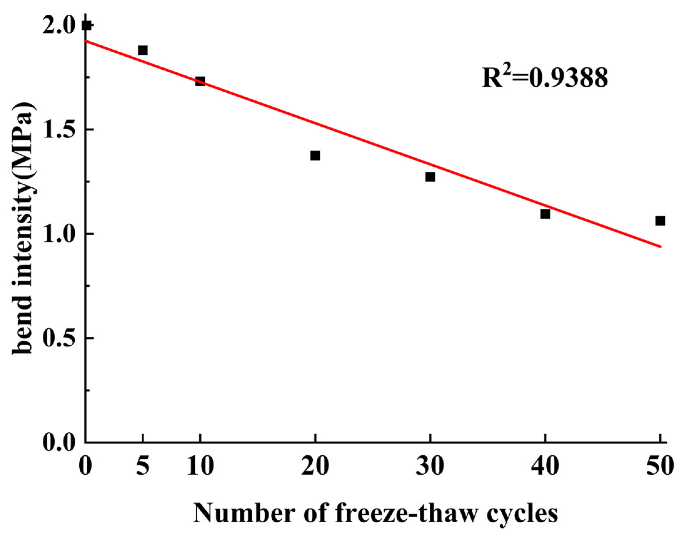
| bend intensity (MPa) | 1.99 | 1.88 | 1.73 | 1.37 | 1.27 | 1.09 | 1.06 |
| Stress Level | 0.6 | 0.68 | 0.76 | 0.84 |
|---|---|---|---|---|
| fatigue life (times) | 323825 | 86809 | 40684 | 3338 |
| Number of Freeze–Thaw Cycles | Stress Ratio | |||
|---|---|---|---|---|
| 0.6 | 0.68 | 0.76 | 0.84 | |
| 0 | 323,825 | 86,809 | 40,684 | 3338 |
| 5 | 303,646 | 77,938 | 35,808 | 2799 |
| 10 | 278,759 | 71,946 | 30,871 | 2098 |
| 20 | 226,268 | 58,921 | 23,902 | 1270 |
| 30 | 164,722 | 36,354 | 11,731 | 696 |
| 40 | 115,890 | 26,134 | 7643 | 463 |
| 50 | 93,516 | 20,034 | 4958 | 283 |
| Type of Analogue Unit | Coupling Mode of Action in the Unit |
|---|---|
| Light load fatigue | Fatigue loading 15,690 times |
| Light load coupling | Fatigue loading 15,690 times and freeze–thaw cycle 10 times |
| Heavy load fatigue | Fatigue loading 21,590 times |
| Heavy load coupling | Fatigue loading 21,590 times and freeze–thaw cycle 10 times |
| Simulated Action Unit (Year) | Light Load Fatigue (MPa) | Light Load Coupling (MPa) | Heavy Load Fatigue (MPa) | Heavy Load Coupling (MPa) |
|---|---|---|---|---|
| 0 | 8311 | 8311 | 8311 | 8311 |
| 1 | 7887 | 5275 | 7792 | 4886 |
| 2 | 7413 | 4262 | 7161 | 3446 |
| 3 | 7090 | 3934 | 6580 | 2945 |
| 4 | 6912 | 3684 | 6437 | 2751 |
| 5 | 6500 | 3316 | 6265 | 2589 |
| Operating Mode | Regression Equation | |
|---|---|---|
| Light load fatigue | 0.9907 | |
| Light load coupling | 0.9857 | |
| Heavy load fatigue | 0.9885 | |
| Heavy load coupling | 0.9879 |
Disclaimer/Publisher’s Note: The statements, opinions and data contained in all publications are solely those of the individual author(s) and contributor(s) and not of MDPI and/or the editor(s). MDPI and/or the editor(s) disclaim responsibility for any injury to people or property resulting from any ideas, methods, instructions or products referred to in the content. |
© 2024 by the authors. Licensee MDPI, Basel, Switzerland. This article is an open access article distributed under the terms and conditions of the Creative Commons Attribution (CC BY) license (https://creativecommons.org/licenses/by/4.0/).
Share and Cite
Song, P.-C.; Chen, G.-X.; Chen, Y.-J. Optimizing the Utilization of Steel Slag in Cement-Stabilized Base Layers: Insights from Freeze–Thaw and Fatigue Testing. Materials 2024, 17, 2576. https://doi.org/10.3390/ma17112576
Song P-C, Chen G-X, Chen Y-J. Optimizing the Utilization of Steel Slag in Cement-Stabilized Base Layers: Insights from Freeze–Thaw and Fatigue Testing. Materials. 2024; 17(11):2576. https://doi.org/10.3390/ma17112576
Chicago/Turabian StyleSong, Peng-Cheng, Guo-Xin Chen, and Ying-Jie Chen. 2024. "Optimizing the Utilization of Steel Slag in Cement-Stabilized Base Layers: Insights from Freeze–Thaw and Fatigue Testing" Materials 17, no. 11: 2576. https://doi.org/10.3390/ma17112576