
Fatigue Life Data Fusion Method of Different Stress Ratios Based on Strain Energy Density

Abstract
1. Introduction
2. Methodology
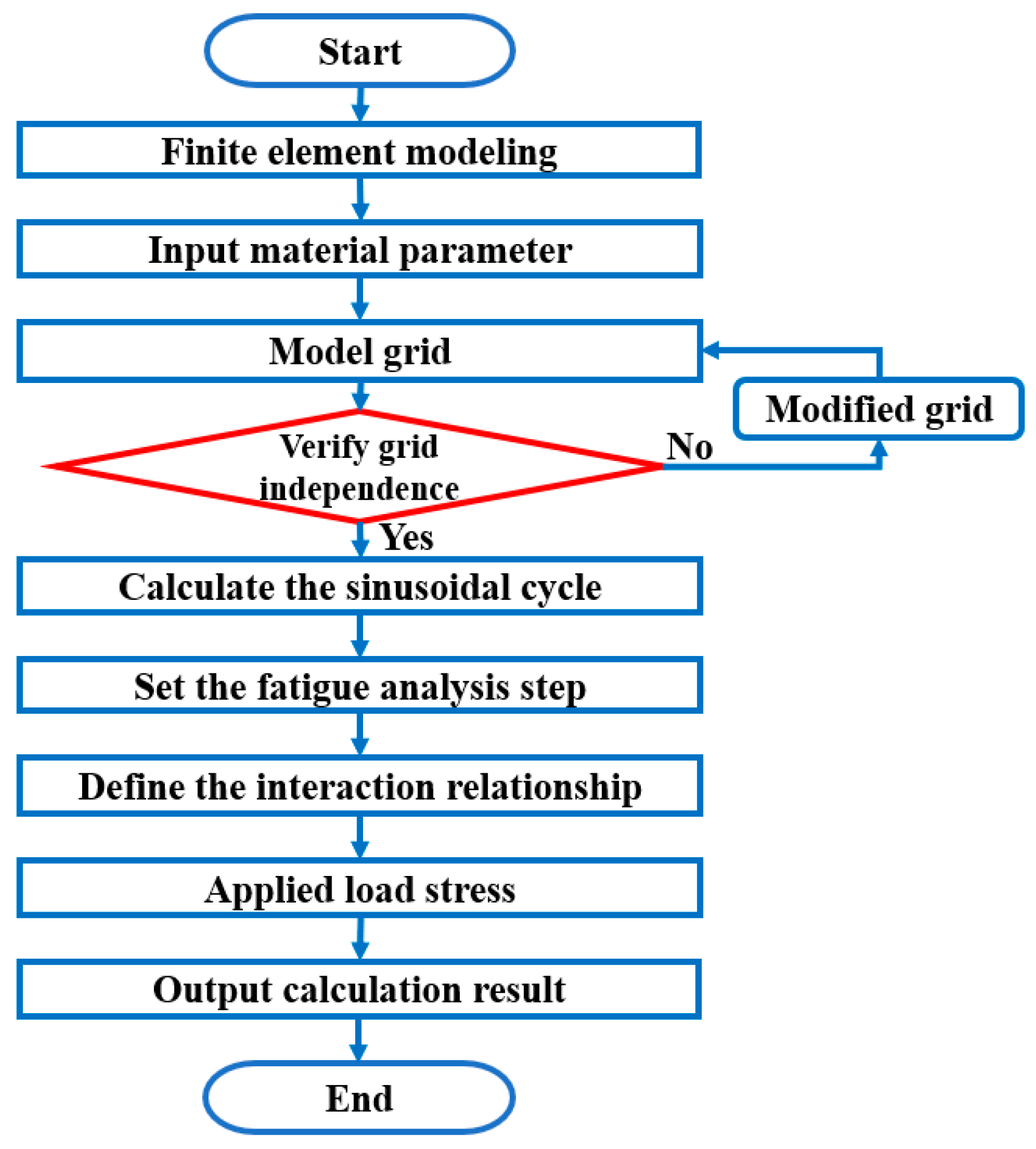
2.1. Strain Energy Density Calculation Method

- (1)
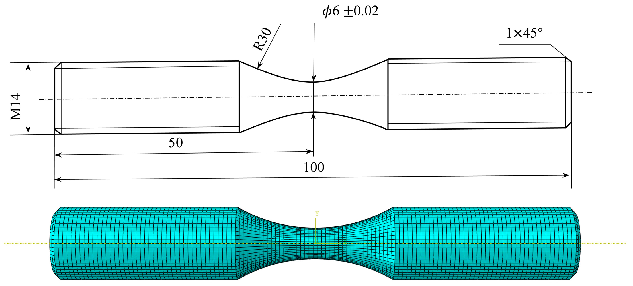
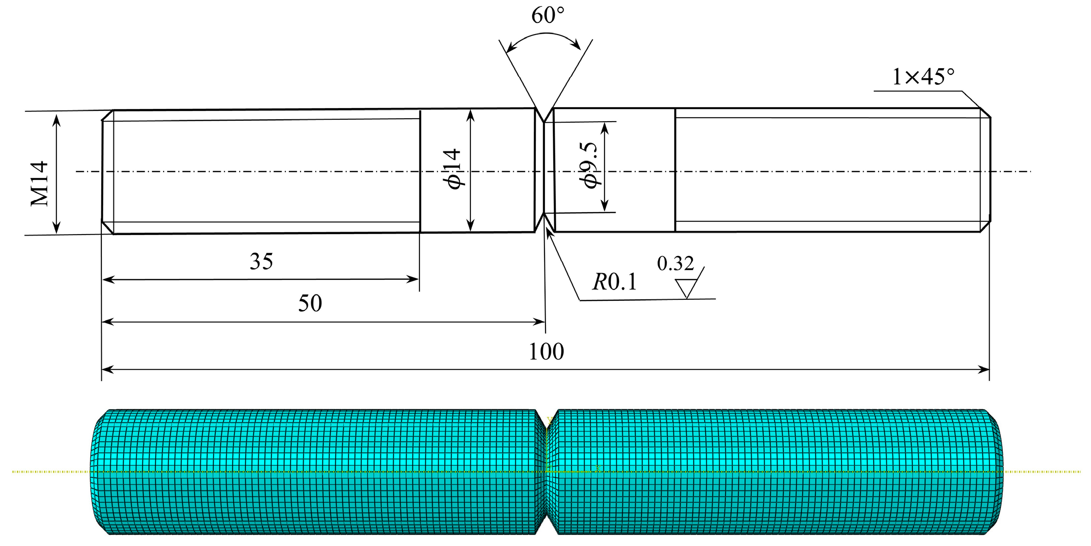
- Finite element modeling based on test specimens;
- (2)
- Inputting the elastic and plastic parameters of the material;
- (3)
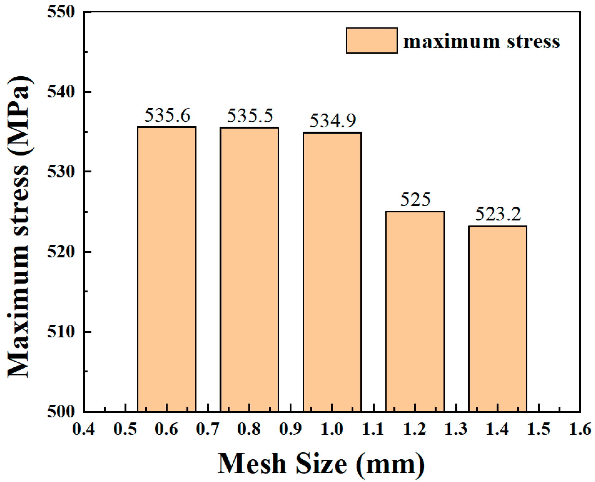
- Dividing the model mesh and verifying mesh independence;
- (4)
- Selecting the number of fatigue cycles and calculating the sinusoidal cycle curve based on the number of cycles and stress ratio;
- (5)
- Applying the sinusoidal cyclic load to the specimen and obtaining the calculation results.
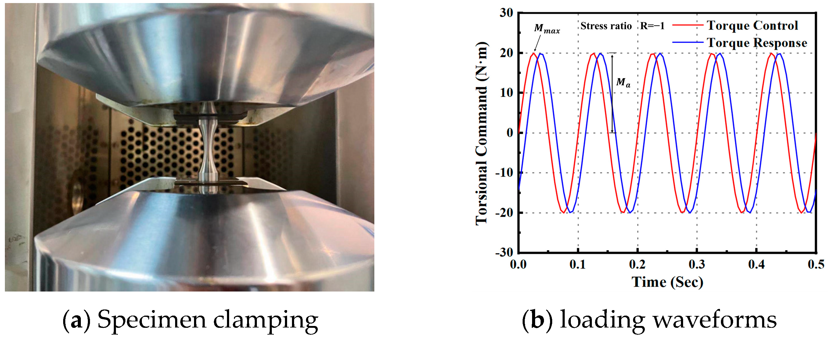
2.2. Torsional Fatigue Test Method and Data
2.3. - Curve and P-- Curve Calculation Method
2.4. Data Fusion Method
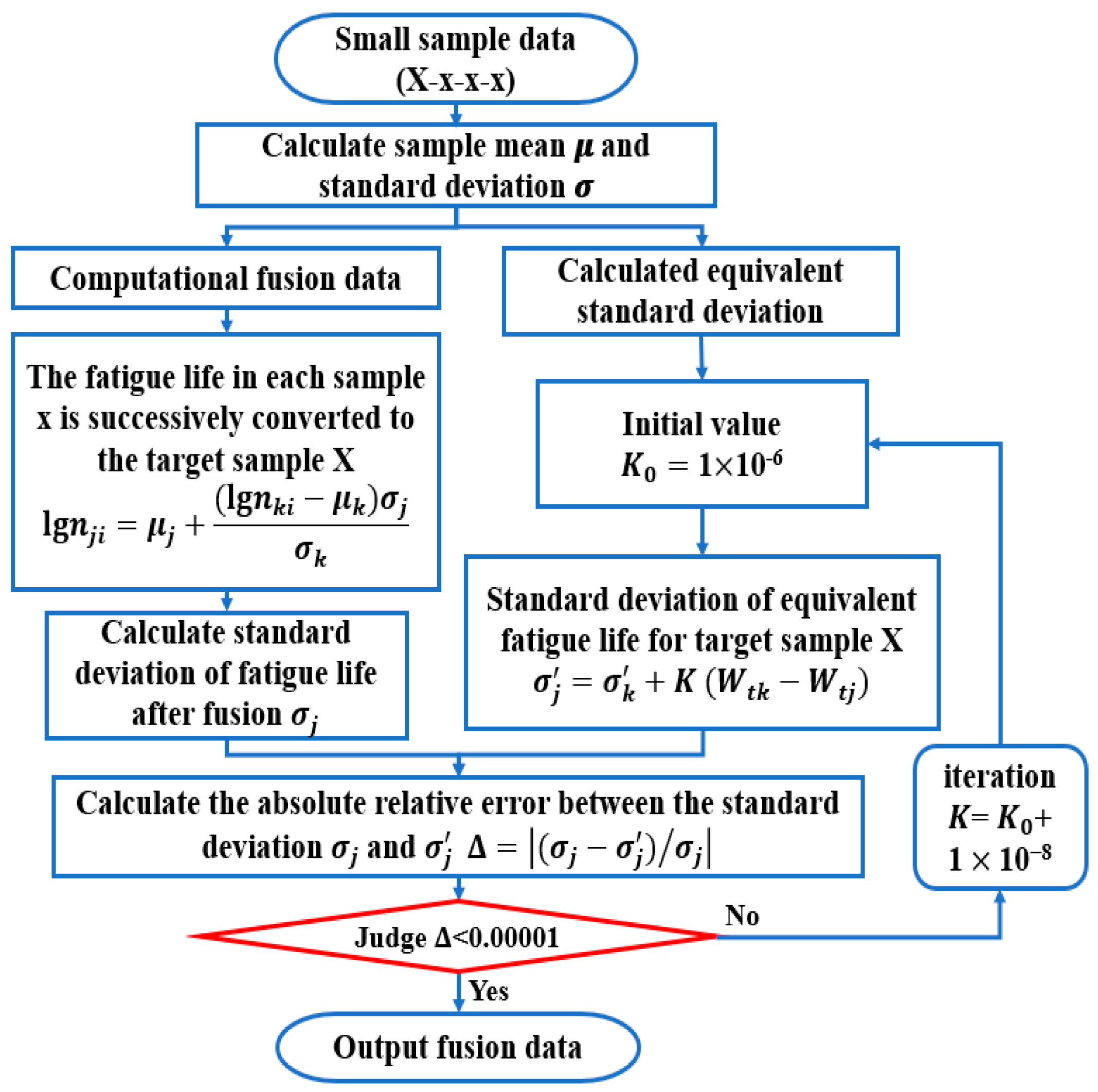
- (1)
- Calculating the mean logarithmic fatigue life of each strain energy density level;
- (2)
- Calculating the logarithmic life standard deviation of the fusion target level;
- (3)
- Fusing data from other strain energy density levels and calculating the standard deviation of the fused life data;
- (4)
- Setting an initial value of and calculating the equivalent standard deviation from other levels to the target level;
- (5)
- Calculating the relative error of two standard deviations. When meets the error requirement, the fusion result is the output.
3. Results and Discussion
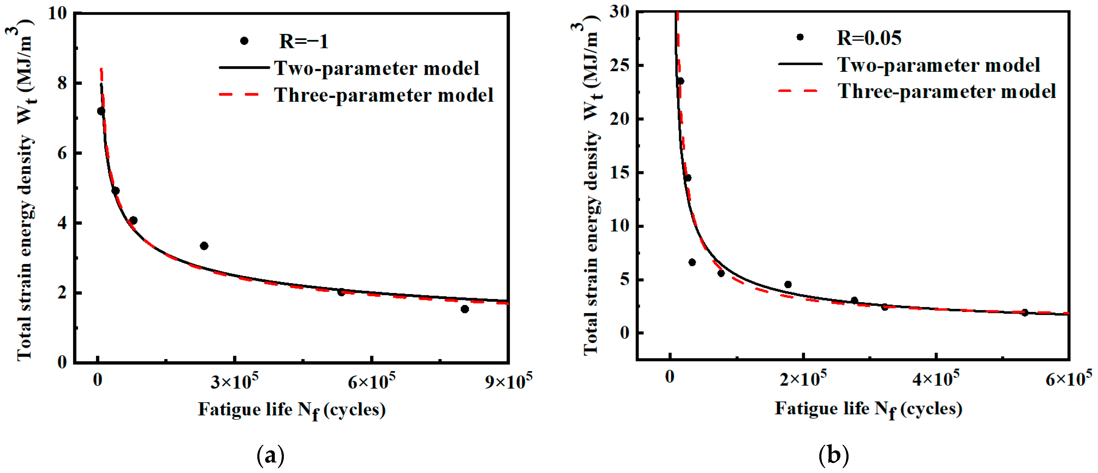
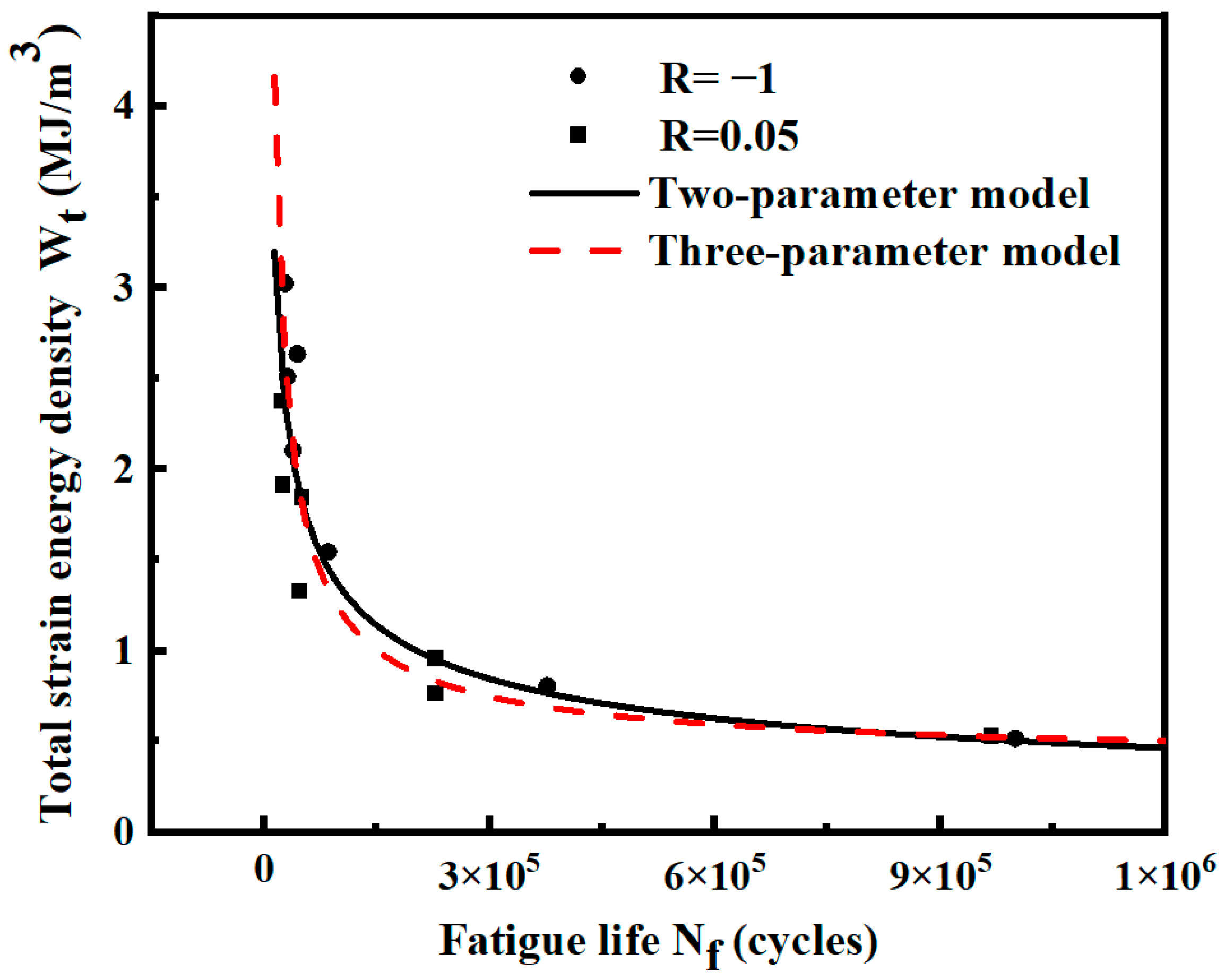
3.1. - Curve Fitting from Test Data
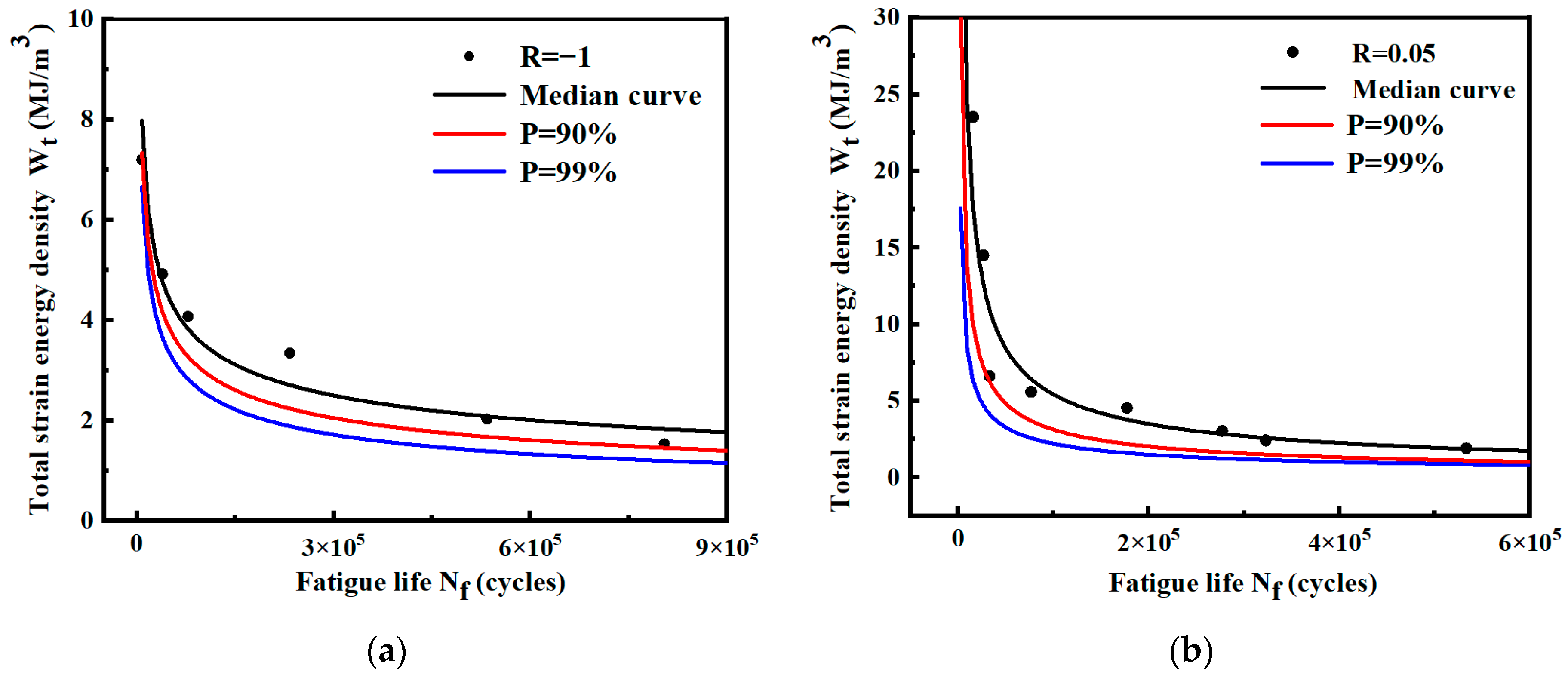
3.2. P-- Curve Fitting
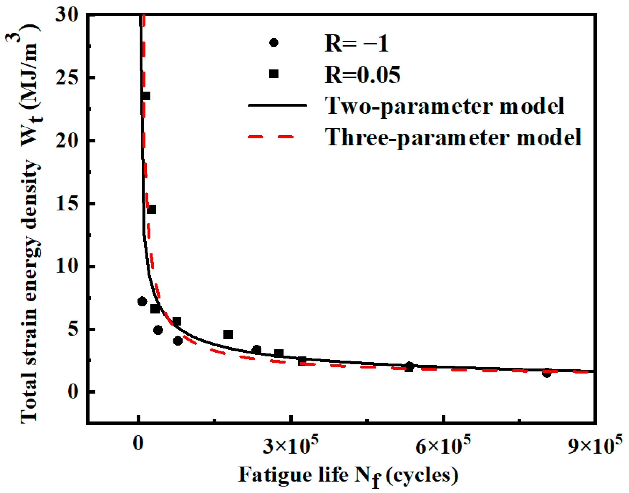
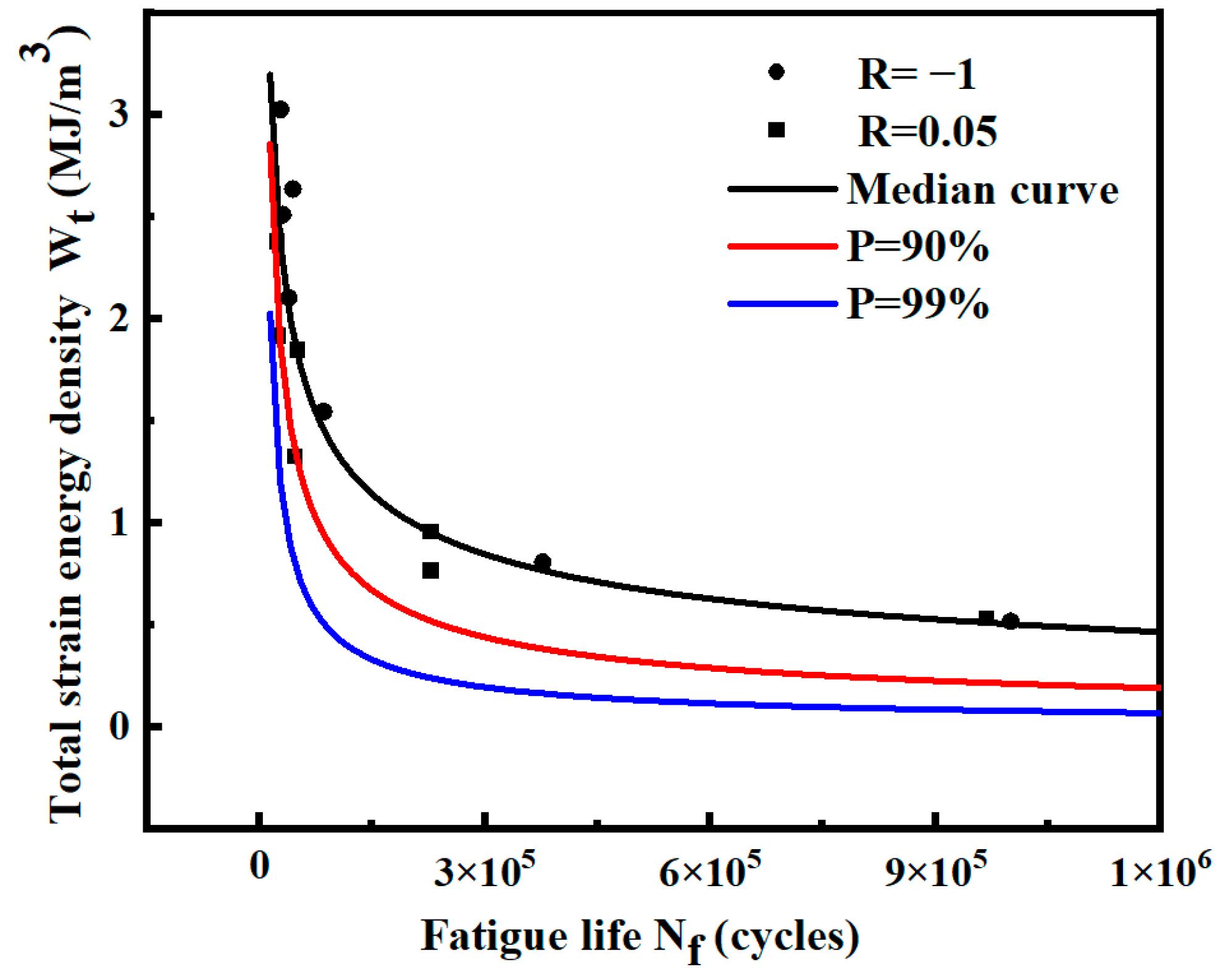
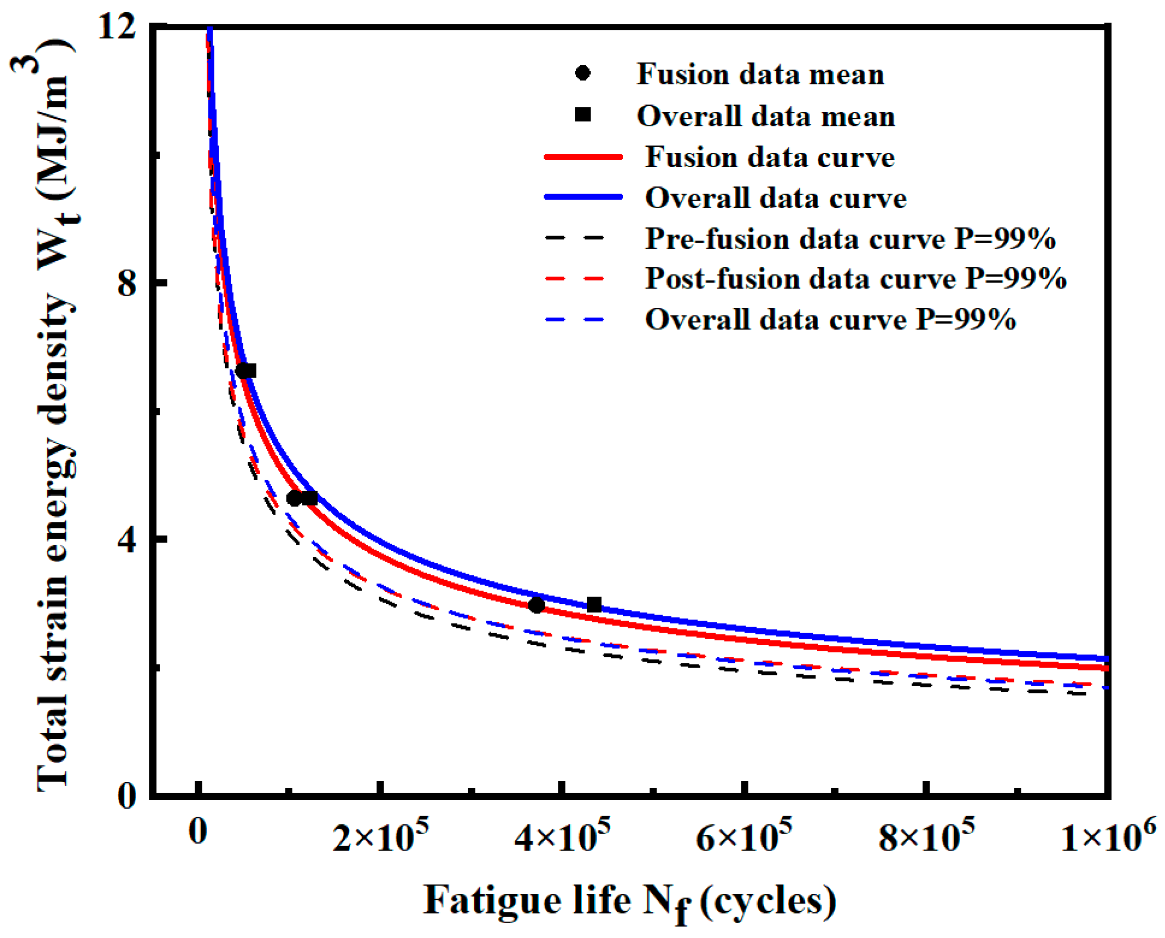
3.3. Data Fusion and P-- Curve Fitting Based on the Overall Data
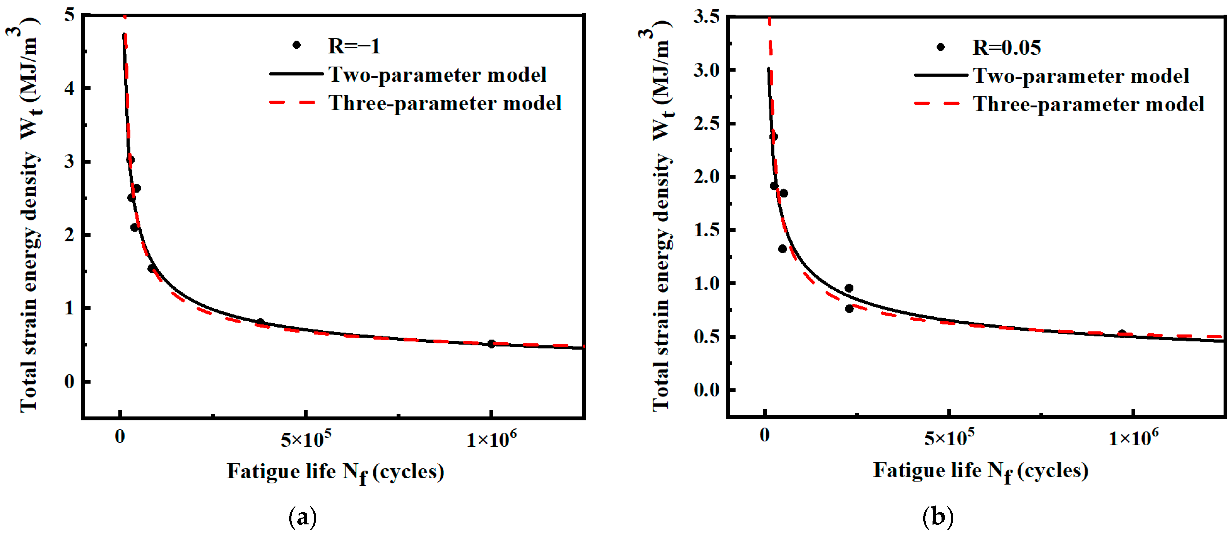
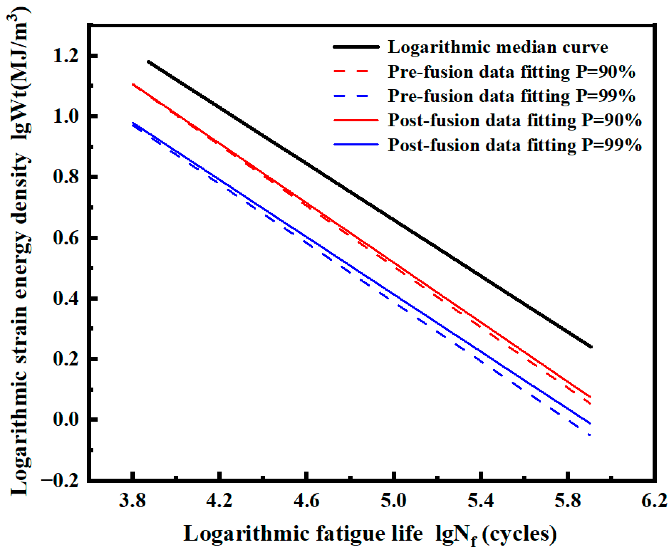
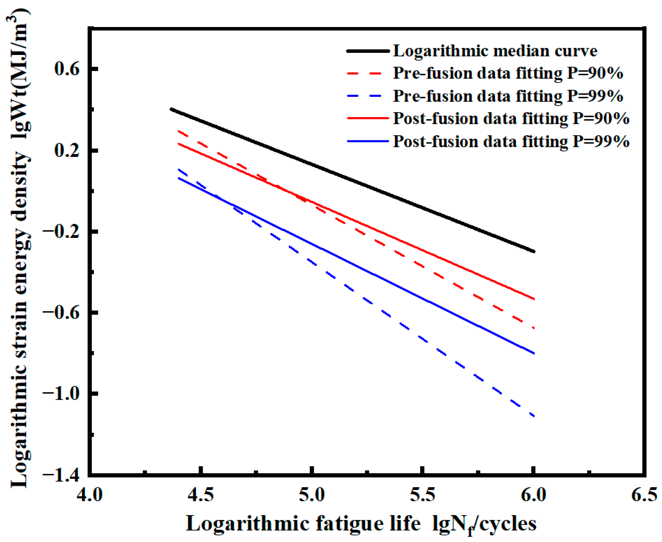
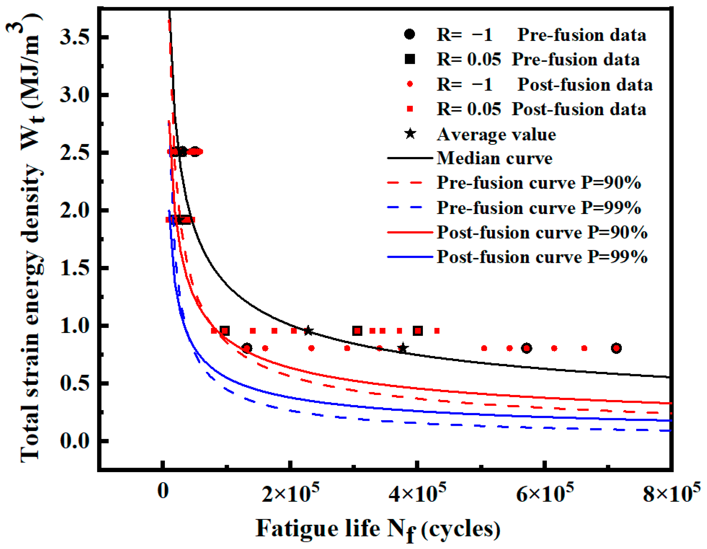
3.4. Data Fusion and P-- Curve Fitting under Different Stress Ratios
4. Conclusions
- (1)
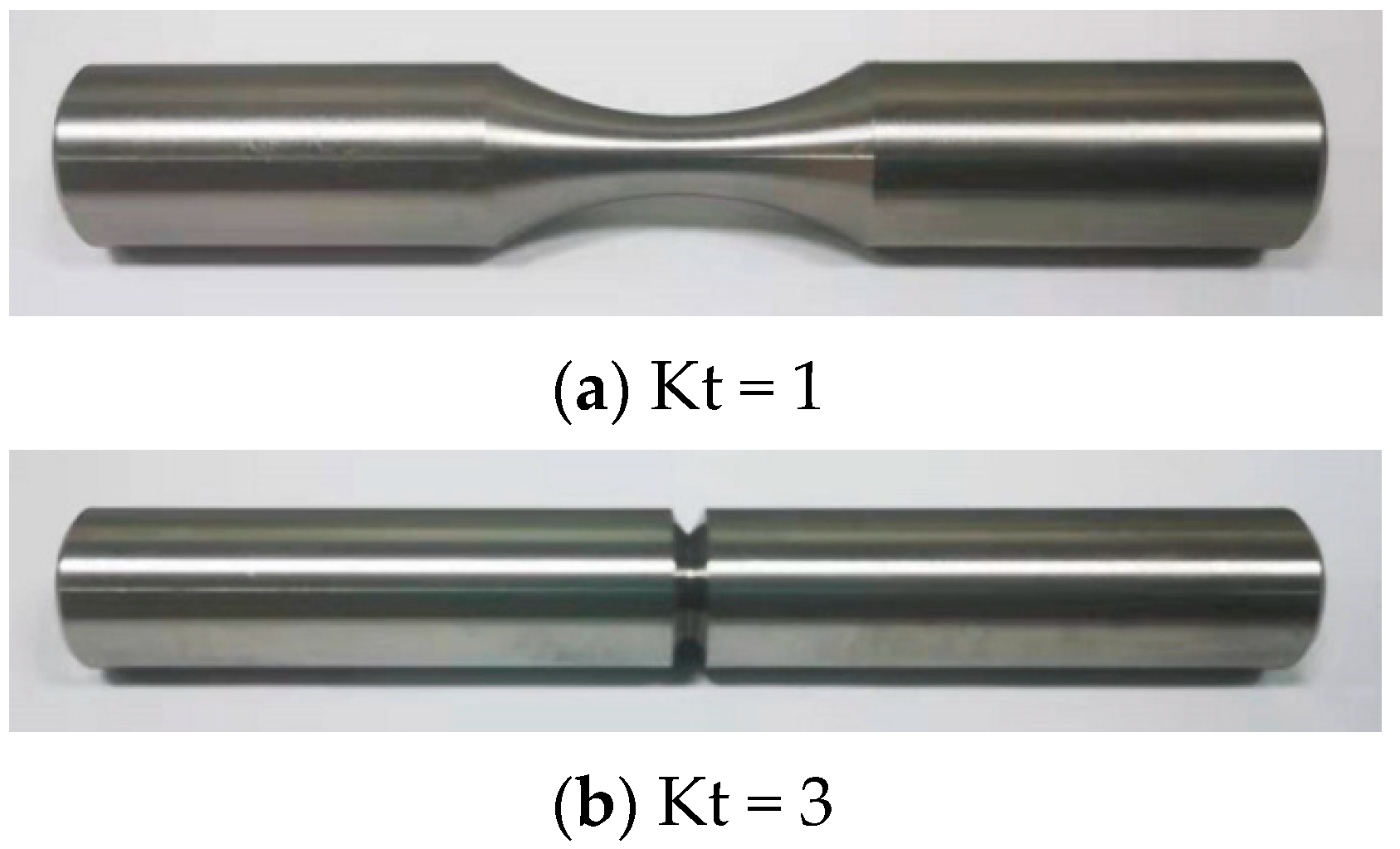
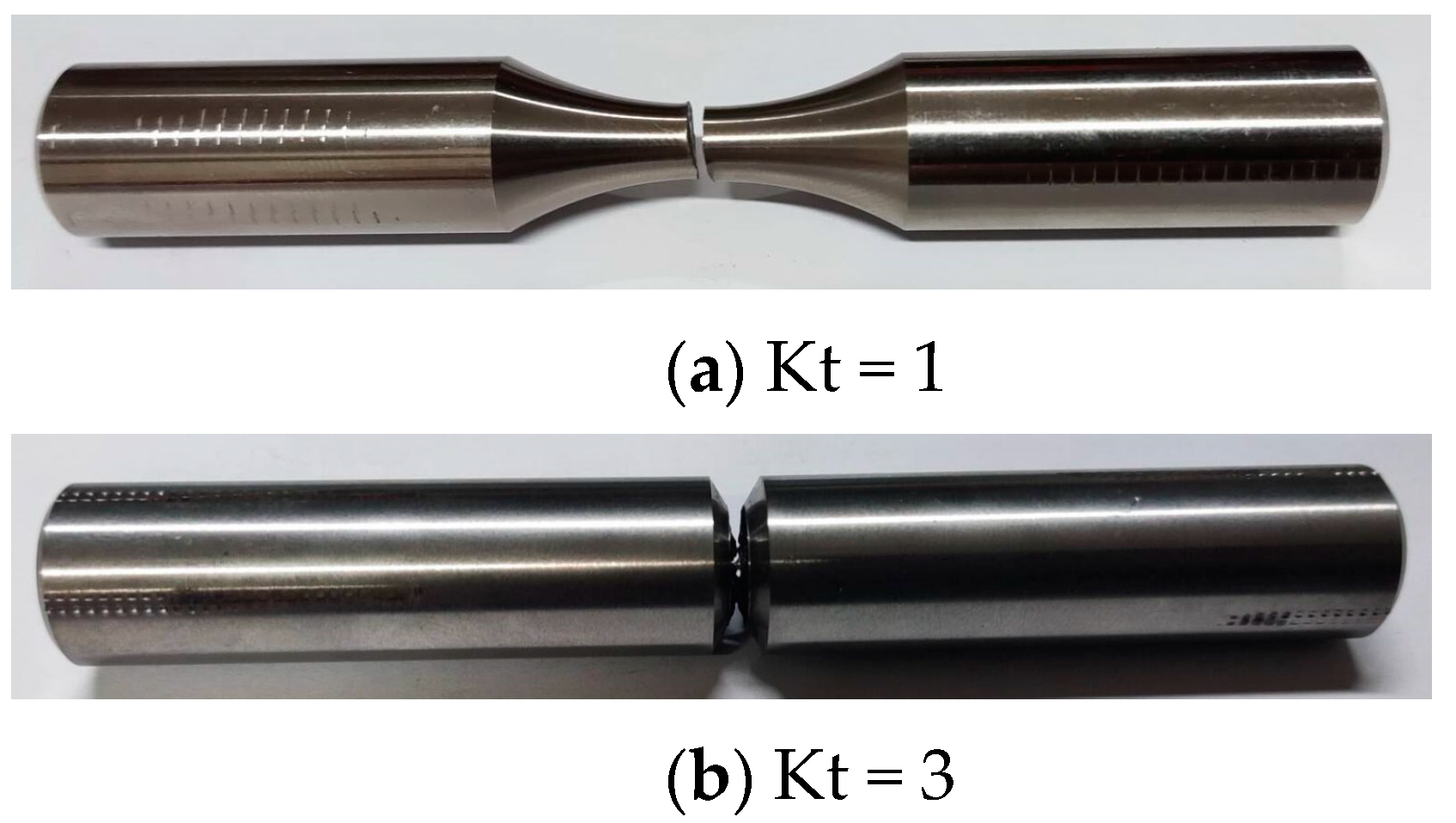
- Torsional fatigue tests were conducted, and test data were obtained. Based on numerical simulation, a method for the calculation of strain energy density was established. And the strain energy densities of specimens under different working conditions were calculated to provide a database for subsequent studies.
- (2)
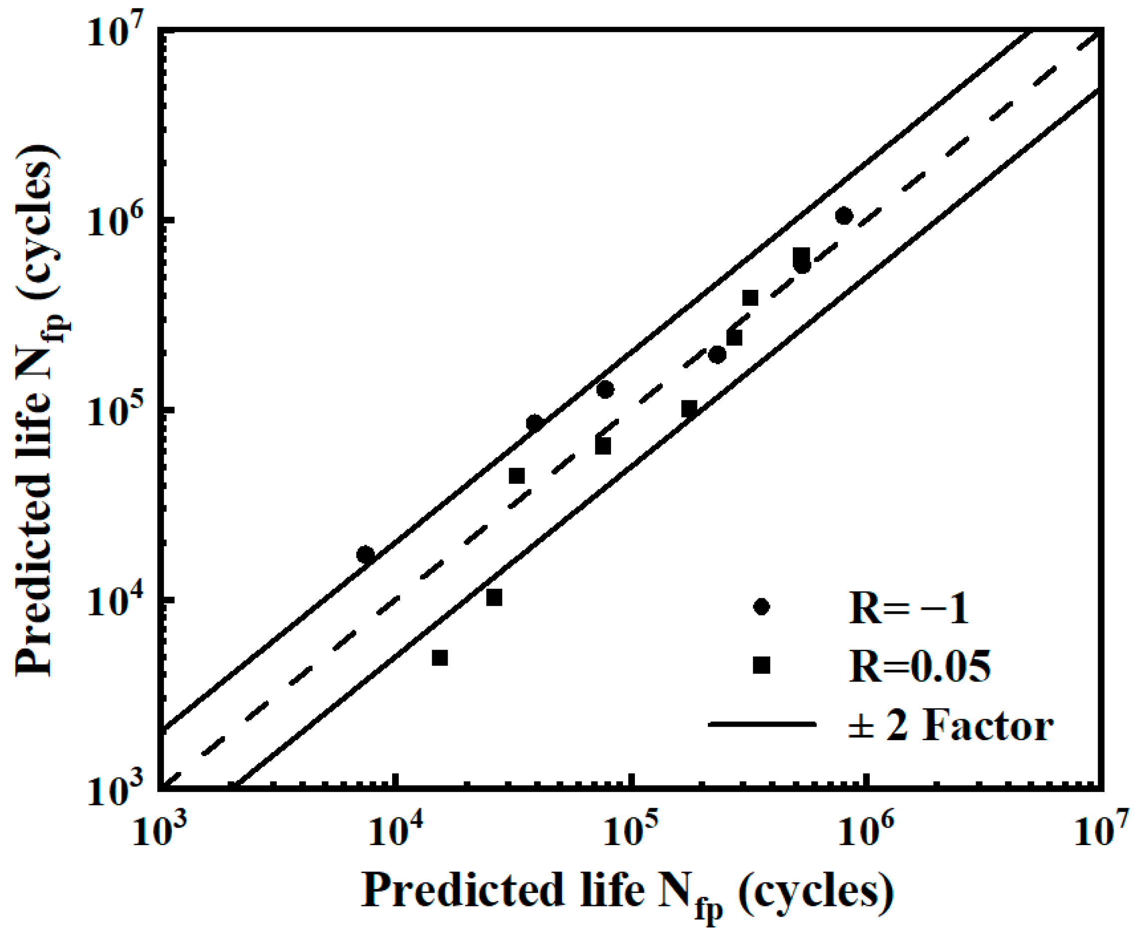
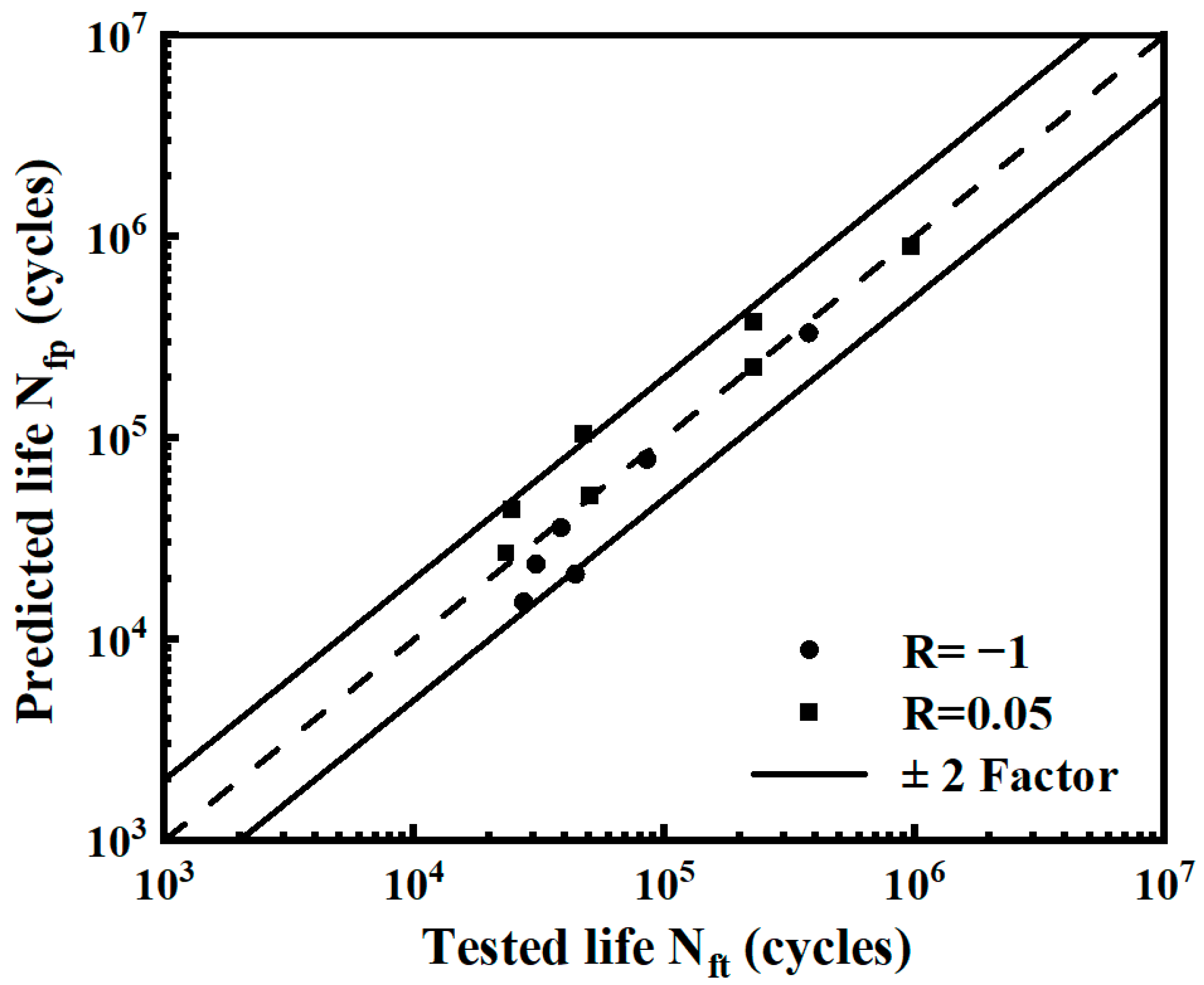
- The - and P-- prediction models under two different stress ratios were fitted. By error analysis, more than 85% of the data were distributed within the ±2 scatter bands, which verified the homogeneity of the models under different stress ratios.
- (3)
- A data fusion method for fatigue life under different stress ratios was proposed. The data fusion method can expand small sample data, significantly reducing the standard deviation of medium and low strain energy density levels. Compared with the pre-fusion data, the standard deviation of the post-fusion data was reduced by a maximum of 21.5% for the smooth specimens and 38.5% for the notched specimens. The life prediction accuracy of the fused P-- curves increased.
Author Contributions
Funding
Institutional Review Board Statement
Informed Consent Statement
Data Availability Statement
Conflicts of Interest
Nomenclature
| S | fatigue stress | cyclic strain hardening index | |
| N | fatigue life | cyclic strength coefficient | |
| P | survival rate | temperature | |
| strain energy density | Kt | stress concentration factor | |
| elastic strain energy density | R | stress ratio | |
| plastic strain energy density | Poisson ratio | ||
| strain | average fatigue life | ||
| stress | probabilistic fatigue life | ||
| Maximum stress | one-side tolerance factor | ||
| strain range | fatigue life of specimen at strain energy density level | ||
| stress range | probability of life being less than at strain energy density level | ||
| plastic strain | Mean fatigue life at strain energy density level | ||
| elastic strain | standard deviation at strain energy density level | ||
| elastic modulus |
References
- Murakami, Y.; Yokoyama, N.N.; Nagata, J. Mechanism of fatigue failure in ultralong life regime. Fatigue Fract. Eng. Mater. Struct. 2002, 25, 735–746. [Google Scholar] [CrossRef]
- Kocańda, S. Fatigue Failure of Metals; Springer: Dordrecht, The Netherlands, 1978. [Google Scholar]
- Li, W.; Yan, Q.; Xue, J. Analysis of a crankshaft fatigue failure. Eng. Fail. Anal. 2015, 55, 139–147. [Google Scholar] [CrossRef]
- Bhaumik, S.; Sujata, M.; Venkataswamy, M. Fatigue failure of aircraft components. Eng. Fail. Anal. 2008, 15, 675–694. [Google Scholar] [CrossRef]
- Yang, J.; Gong, Y.; Jiang, L.; Lin, W.; Liu, H. A multi-axial and high-cycle fatigue life prediction model based on critical plane criterion. J. Mater. Res. Technol. 2022, 18, 4549–4563. [Google Scholar] [CrossRef]
- Jiang, L.; Zhang, Y.; Gong, Y.; Li, W.; Ren, S.; Liu, H. A new model characterizing the fatigue delamination growth in DCB laminates with combined effects of fiber bridging and stress ratio. Compos. Struct. 2021, 268, 113943. [Google Scholar] [CrossRef]
- Lee, Y.L.; Barkey, M.E.; Kang, H.T. Metal Fatigue Analysis Handbook: Practical Problem-Solving Techniques for Computer-Aided Engineering; Elsevier: Amsterdam, The Netherlands, 2011. [Google Scholar]
- Shao, Y.; Lu, P.; Wang, B.; Xiang, Q. Fatigue reliability assessment of small sample excavator working devices based on Bootstrap method. Frat. Ed Integrità Strutt. 2019, 13, 757–767. [Google Scholar] [CrossRef]
- Nie, T. Application of small sample analysis in life estimation of aeroengine components. J. Southwest Jiaotong Univ. 2010, 18, 285–288. [Google Scholar]
- Xie, L.; Liu, J.; Wu, N.; Qian, W. Probabilistic Specimen Property-Fatigue Life Mapping and P-S-N Curve Fitting. Int. J. Reliab. Qual. Saf. Eng. 2013, 20, 1350020. [Google Scholar] [CrossRef]
- Xie, L.; Liu, J.; Wu, N.; Qian, W. Backwards statistical inference method for P–S–N curve fitting with small-sample experiment data. Int. J. Fatigue 2014, 63, 62–67. [Google Scholar] [CrossRef]
- Chen, J.; Liu, S.; Zhang, W.; Liu, Y. Uncertainty quantification of fatigue S-N curves with sparse data using hierarchical Bayesian data augmentation. Int. J. Fatigue 2020, 134, 105511. [Google Scholar] [CrossRef]
- Liu, X.-W.; Lu, D.-G.; Hoogenboom, P.C. Hierarchical Bayesian fatigue data analysis. Int. J. Fatigue 2017, 100, 418–428. [Google Scholar] [CrossRef]
- Gao, J.; Yuan, Y. Small sample test approach for obtaining P-S-N curves based on a unified mathematical model. Proc. Inst. Mech. Eng. Part C J. Mech. Eng. Sci. 2020, 234, 4751–4760. [Google Scholar] [CrossRef]
- Li, C.; Wu, S.; Zhang, J.; Xie, L.; Zhang, Y. Determination of the fatigue P-S-N curves—A critical review and improved backward statistical inference method. Int. J. Fatigue 2020, 139, 105789. [Google Scholar] [CrossRef]
- Klemenc, J.; Fajdiga, M. Estimating S–N curves and their scatter using a differential ant-stigmergy algorithm. Int. J. Fatigue 2012, 43, 90–97. [Google Scholar] [CrossRef]
- Shimizu, S.; Tosha, K.; Tsuchiya, K. New data analysis of probabilistic stress-life (P–S–N) curve and its application for structural materials. Int. J. Fatigue 2010, 32, 565–575. [Google Scholar] [CrossRef]
- Bell, J. The Experimental Foundations of Solid Mechanics; Spinger: New York, NY, USA, 1973; pp. 5–120. [Google Scholar]
- Inglis, N.P. Hysteresis and fatigue of Wohler rotating cantilever specimen. Metallurgist 1927, 1, 23–27. [Google Scholar]
- Miner, M.A. Cumulative damage in fatigue. J. Appl. Mech. 1945, 12, 159–164. [Google Scholar] [CrossRef]
- Lazzarin, P.; Zambardi, R. A finite-volume-energy based approach to predict the static and fatigue behavior of components with sharp V-shaped notches. Int. J. Fract. 2001, 112, 275–298. [Google Scholar] [CrossRef]
- Branco, R.; Prates, P.; Costa, J.; Borrego, L.; Berto, F.; Kotousov, A.; Antunes, F. Rapid assessment of multiaxial fatigue lifetime in notched components using an averaged strain energy density approach. Int. J. Fatigue 2019, 124, 89–98. [Google Scholar] [CrossRef]
- Braccesi, C.; Morettini, G.; Cianetti, F.; Palmieri, M. Development of a new simple energy method for life prediction in multiaxial fatigue. Int. J. Fatigue 2018, 112, 1–8. [Google Scholar] [CrossRef]
- McCartney, L. Energy methods for fatigue damage modelling of laminates. Compos. Sci. Technol. 2008, 68, 2601–2615. [Google Scholar] [CrossRef]
- Cao, X.; Tang, X.; Chen, L.; Wang, D.; Jiang, Y. Study on Characteristics of Failure and Energy Evolution of Different Moisture-Containing Soft Rocks under Cyclic Disturbance Loading. Materials 2024, 17, 1770. [Google Scholar] [CrossRef] [PubMed]
- Tavernelli, J.F.; Coffi, L.F., Jr. Experimental support for generalized equation predicting low cycle fatigue. J. Basic Eng. 1962, 84, 533. [Google Scholar] [CrossRef]
- Manson, S.S. Fatigue: A complex subject—Some simple approximations. Exp. Mech. 1965, 5, 193–226. [Google Scholar] [CrossRef]
- Hu, Z.; Berto, F.; Hong, Y.; Susmel, L. Comparison of TCD and SED methods in fatigue lifetime assessment. Int. J. Fatigue 2019, 123, 105–134. [Google Scholar] [CrossRef]
- Fan, Y.-N.; Shi, H.-J.; Tokuda, K. A generalized hysteresis energy method for fatigue and creep-fatigue life prediction of 316L(N). Mater. Sci. Eng. A 2015, 625, 205–212. [Google Scholar] [CrossRef]
- Hwang, J.H.; Kim, D.W.; Lim, J.Y.; Hong, S.G. Energy-Based Unified Models for Predicting the Fatigue Life Behaviors of Austenitic Steels and Welded Joints in Ultra-Supercritical Power Plants. Materials 2024, 17, 2186. [Google Scholar] [CrossRef] [PubMed]
- Liao, D.; Zhu, S.-P. Energy field intensity approach for notch fatigue analysis. Int. J. Fatigue 2019, 127, 190–202. [Google Scholar] [CrossRef]
- Song, W.; Liu, X.; Zhou, G.; Wei, S.; Shi, D.; He, M.; Berto, F. Notch energy-based low and high cycle fatigue assessment of load-carrying cruciform welded joints considering the strength mismatch. Int. J. Fatigue 2021, 151, 106410. [Google Scholar] [CrossRef]
- Berto, F. Fatigue and fracture assessment of notched components by means of the Strain Energy Density. Eng. Fract. Mech. 2016, 167, 176–187. [Google Scholar] [CrossRef]
- El Kadi, H.; Ellyin, F. Effect of stress ratio on the fatigue of unidirectional glass fiber/epoxy composite laminae. Composites 1994, 25, 917–924. [Google Scholar] [CrossRef]
- Kujawski, D.; Ellyin, F. A unified approach to mean stress effect on fatigue threshold conditions. Int. J. Fatigue 1995, 17, 101–106. [Google Scholar] [CrossRef]
- Ellyin, F. Fatigue Damage, Crack Growth and Life Prediction; Springer: Berlin/Heidelberg, Germany, 2012. [Google Scholar]
- Skelton, R.P. Cyclic stress-strain properties during high strain fatigue. In High Temperature Fatigue: Properties and Prediction; Springer: Dordrecht, The Netherlands, 1987; pp. 27–112. [Google Scholar]
- Zhu, S.-P.; Huang, H.-Z.; He, L.-P.; Liu, Y.; Wang, Z. A generalized energy-based fatigue–creep damage parameter for life prediction of turbine disk alloys. Eng. Fract. Mech. 2012, 90, 89–100. [Google Scholar] [CrossRef]
- Li, X.K.; Chen, S.; Zhu, S.P.; Liao, D.; Gao, J.W. Probabilistic fatigue life prediction of notched components using strain energy density approach. Eng. Fail. Anal. 2021, 124, 105375. [Google Scholar] [CrossRef]
- Klesnil, M.; Lukác, P. Fatigue of Metallic Materials; Elsevier: Amsterdam, The Netherlands, 1992. [Google Scholar]
- Branco, R.; Costa, J.D.; Berto, F.; Antunes, F.V. Fatigue life assessment of notched round bars under multiaxial loading based on the total strain energy density approach. Theor. Appl. Fract. Mech. 2018, 97, 340–348. [Google Scholar] [CrossRef]
- Zhang, S.; Zhao, D. (Eds.) Aerospace Materials Handbook; CrC Press: Boca Raton, FL, USA, 2012. [Google Scholar]
- Golos, K.; Ellyin, F. A Total Strain Energy Density Theory for Cumulative Fatigue Damage. J. Press. Vessel. Technol. 1988, 110, 36–41. [Google Scholar] [CrossRef]
- Sun, J.; Yang, Z.; Chen, G. Research on three-parameter power function equivalent energy method for high temperature strain fatigue. In Proceedings of the 2010 the 2nd International Conference on Industrial Mechatronics and Automation, Wuhan, China, 30–31 May 2010; Volume 1, pp. 84–87. [Google Scholar]
- Makepeace, C.E.; Ailor, W.H. Statistical Design of Experiments. In Handbook on Corrosion Testing and Evaluation; Jogn Wiley & Sons Inc.: Hoboken, NJ, USA, 1971. [Google Scholar]
- Tanaka, S.; Ichikawa, M.; Akita, S. A probabilistic investigation of fatigue life and cumulative cycle ratio. Eng. Fract. Mech. 1984, 20, 501–513. [Google Scholar] [CrossRef]


| (°C) | (GPa) | ||
|---|---|---|---|
| 20 | 109 | 0.34 | 0.07 |
| TC4 Alloy, T = 20 °C, Kt = 1, R = −1 | ||||
|---|---|---|---|---|
| Maximum Stress σmax/MPa | Fatigue Life /Cycles | Reference Strain Energy Density /(MJ/m3) | Calculated Strain Energy Density /(MJ/m3) | Relative Error |
| 780 | 4443 | 12 | 11.7581 | −2.02% |
| 730 | 6262 | 10.3 | 10.32782 | 0.27% |
| 680 | 8725 | 8.85 | 8.79789 | −0.59% |
| 630 | 12,441 | 7.63 | 7.56113 | −0.90% |
| 580 | 18,028 | 6.46 | 6.49351 | 0.52% |
| 520 | 28,447 | 5.21 | 5.10411 | −2.03% |
| (°C) | (GPa) | ||
|---|---|---|---|
| 25 | 196.6 | 0.302 | 0.07 |
| Stress Ratio R | Maximum Stress σmax/MPa | Logarithmic Median Life /Cycles | Strain Energy Density /(MJ/m3) |
|---|---|---|---|
| −1 | 700 | 7447 | 7.2057 |
| −1 | 600 | 39,084 | 4.9239 |
| −1 | 550 | 77,983 | 4.0795 |
| −1 | 500 | 232,809 | 3.3485 |
| −1 | 400 | 533,335 | 2.0273 |
| −1 | 350 | 803,526 | 1.5393 |
| 0.05 | 1100 | 15,524 | 23.5288 |
| 0.05 | 1000 | 26,363 | 14.5014 |
| 0.05 | 900 | 32,885 | 6.6179 |
| 0.05 | 850 | 76,560 | 5.5978 |
| 0.05 | 800 | 177,419 | 4.5450 |
| 0.05 | 700 | 276,694 | 3.0503 |
| 0.05 | 650 | 322,833 | 2.4364 |
| 0.05 | 600 | 533,188 | 1.9197 |
| Stress Ratio R | Maximum Stress σmax/MPa | Logarithmic Median Life /Cycles | Strain Energy Density /(MJ/m3) |
|---|---|---|---|
| −1 | 500 | 27,356 | 3.0272 |
| −1 | 450 | 44,030 | 2.6378 |
| −1 | 400 | 30,654 | 2.5113 |
| −1 | 350 | 38,493 | 2.1038 |
| −1 | 300 | 85,066 | 1.5463 |
| −1 | 250 | 376,897 | 0.8068 |
| −1 | 200 | 1,000,000 | 0.5165 |
| 0.05 | 700 | 23,287 | 2.3784 |
| 0.05 | 650 | 24,578 | 1.9174 |
| 0.05 | 600 | 50,506 | 1.8471 |
| 0.05 | 550 | 47,405 | 1.3267 |
| 0.05 | 500 | 227,879 | 0.9575 |
| 0.05 | 450 | 228,355 | 0.7662 |
| 0.05 | 400 | 968,486 | 0.5294 |
| Model Type | Different Stress Ratio Conditions | Model Expression | R2 Value | Predicted Life of Different Strain Energy Densities/Cycles | |
|---|---|---|---|---|---|
| 5 MJ/m3 | 3 MJ/m3 | ||||
| Two-parameter model | R = −1 | = 133.65()−0.315 | 0.94 | 33,897 | 171,568 |
| R = 0.05 | = 7793.28()−0.631 | 0.92 | 114,769 | 257,875 | |
| R = −1 and 0.05 | = 932.65()−0.462 | 0.85 | 82,232 | 248,446 | |
| Three-parameter model | R = −1 | = 167.07()−0.335 | 0.94 | 35,403 | 162,658 |
| R = 0.05 | = 99797.05()−0.883 + 1.10 | 0.91 | 98,205 | 221,731 | |
| R = −1 and 0.05 | = 40616.28()−0.825 + 1.10 | 0.83 | 74,107 | 177,182 | |
| Model Type | Different Stress Ratio Conditions | Model Expression | R2 Value | Predicted Life of Different Strain Energy Densities/Cycles | |
|---|---|---|---|---|---|
| 2 MJ/m3 | 1 MJ/m3 | ||||
| Two-parameter model | R = −1 | = 355.959()−0.474 | 0.97 | 55,926 | 241,379 |
| R = 0.05 | = 95.649()−0.380 | 0.94 | 26,311 | 163,049 | |
| R = −1 and 0.05 | = 189.54()−0.429 | 0.91 | 40,516 | 203,857 | |
| Three-parameter model | R = −1 | = 1472.68()−0.617 + 0.23 | 0.97 | 54,050 | 208,289 |
| R = 0.05 | = 942.00()−0.614 + 0.33 | 0.94 | 30,269 | 133,967 | |
| R = −1 and 0.05 | = 4631.96()−0.747 + 0.37 | 0.89 | 42,001 | 149,946 | |
| Different Stress Ratio Conditions | Probability Level | Model Expression |
|---|---|---|
| R = −1 | = 90% | = 162.31()−0.347 |
| = 99% | = 178.43()−0.368 | |
| R = 0.05 | = 90% | = 4026.15()−0.622 |
| = 99% | = 1440.39()−0.563 | |
| R = −1 and 0.05 | = 90% | = 1008.63()−0.500 |
| = 99% | = 657.25()−0.486 |
| Different Stress Ratio Conditions | Probability Level | Model Expression |
|---|---|---|
| R = −1 | = 90% | = 2476.45 ()−0.694 |
| = 99% | = 10476.59()−0.894 | |
| R = 0.05 | = 90% | = 306.27()−0.511 |
| = 99% | = 983.08()−0.657 | |
| R = −1 and 0.05 | = 90% | = 911.55()−0.605 |
| = 99% | = 2775.81()−0.759 |
| Strain Energy Density/(MJ/m3) | Logarithmic Fatigue Life /Cycles |
|---|---|
| 6.639 | 4.624, 4.699, 4.678, 4.713, 4.768 |
| 4.652 | 4.914, 4.992, 5.014, 5.065, 5.127 |
| 2.987 | 5.472, 5.532, 5.560, 5.607, 5.677 |
| Strain Energy Density/(MJ/m3) | Logarithmic Fatigue Life /Cycles |
|---|---|
| 6.639 | 4.624, 4.699, 4.678, 4.713, 4.768, 4.593, 4.653, 4.681, 4.727, 4.798, 4.582, 4.660, 4.682, 4.734, 4.795 |
| 4.652 | 4.914, 4.992, 5.014, 5.065, 5.127, 4.925, 4.985, 5.013, 5.059, 5.130, 4.956, 5.001, 5.010, 5.045, 5.100 |
| 2.987 | 5.472, 5.532, 5.560, 5.607, 5.677, 5.461, 5.539, 5.562, 5.613, 5.674, 5.503, 5.549, 5.558, 5.592, 5.647 |
| Strain Energy Density/(MJ/m3) | Pre-Fusion Fatigue Data /Cycles | Post-Fusion Fatigue Data /Cycles | /Cycles | |||
|---|---|---|---|---|---|---|
| Logarithmic Mean | Logarithmic Standard Deviation | Logarithmic Mean | Logarithmic Standard Deviation | Logarithmic Mean | Logarithmic Standard Deviation | |
| 6.639 | 4.69046 | 0.053750 | 4.69046 | 0.065993 | 4.73836 | 0.067467 |
| 4.652 | 5.02218 | 0.079866 | 5.02218 | 0.065994 | 5.08858 | 0.089017 |
| 2.987 | 5.56984 | 0.077304 | 5.56984 | 0.065995 | 5.63849 | 0.094436 |
| Data Type | Probability Level | Model Expression | Predicted Life of Different Strain Energy Densities and Relative Error Based on Overall Data | |||||
|---|---|---|---|---|---|---|---|---|
| 6.639 MJ/m3 | Relative Error | 4.652 MJ/m3 | Relative Error | 2.987 MJ/m3 | Relative Error | |||
| Pre-fusion data | = 50% | = 438.94()−0.390 | 46,499 | 11.48% | 115,745 | 13.15% | 360,451 | 15.19% |
| = 99% | = 476.12()−0.411 | 32,725 | 6.99% | 77,750 | 7.58% | 228,473 | 8.31% | |
| Post-fusion data | = 50% | = 438.94()−0.390 | 46,499 | 11.48% | 115,745 | 13.15% | 360,451 | 15.19% |
| = 99% | = 381.36()−0.390 | 32,423 | 7.85% | 80,707 | 4.07% | 251,337 | 0.87% | |
| Overall data | = 50% | = 421.98()−0.382 | 52,528 | - | 133,274 | - | 425,031 | - |
| = 99% | = 475.35()−0.408 | 35,184 | - | 84,127 | - | 249,181 | - | |
| Stress Ratio R | Strain Energy Density /(MJ/m3) | /Cycles | Logarithmic Fatigue Life after Fusion /Cycles |
|---|---|---|---|
| −1 | 4.079 | 4.971, 5.039, 4.664 | 4.971, 5.039, 4.664, 4.621, 4.971, 5.083, 4.892, 4.661, 5.122, 5.130, 4.629, 4.916 |
| 2.027 | 5.456, 5.806, 5.919 | 5.456, 5.806, 5.919, 5.807, 5.875, 5.500, 5.727, 5.497, 5.958, 5.965, 5.465, 5.752 | |
| 0.05 | 5.598 | 4.884, 4.653, 5.114 | 4.884, 4.653, 5.114, 4.964, 5.031, 4.656, 4.613, 4.963, 5.076, 5.122, 4.621, 4.908 |
| 3.050 | 5.681, 5.180, 5.467 | 5.681, 5.180, 5.467, 5.522, 5.590, 5.215, 5.171, 5.521, 5.634, 5.442, 5.212, 5.673 |
| Stress Ratio R | Strain Energy Density /(MJ/m3) | Pre-Fusion Data Nf/Cycles | Post-Fusion Data Nf/Cycles | ||
|---|---|---|---|---|---|
| Logarithmic Mean | Logarithmic Standard Deviation | Logarithmic Mean | Logarithmic Standard Deviation | ||
| −1 | 4.079 | 4.88153 | 0.1997664 | 4.88153 | 0.1975206 |
| 2.027 | 5.71650 | 0.2414045 | 5.71650 | 0.1975221 | |
| 0.05 | 5.598 | 4.89483 | 0.2306621 | 4.88483 | 0.1975220 |
| 3.050 | 5.44238 | 0.2513805 | 5.44238 | 0.1975213 | |
| Data Type | Probability Level | Model Expression | Predicted Life of Different Strain /Cycles | |||
|---|---|---|---|---|---|---|
| 5.598 MJ/m3 | 4.079 MJ/m3 | 3.050 MJ/m3 | 2.027 MJ/m3 | |||
| Pre-fusion data | = 90% | = 1008.63()−0.500 | 32,464 | 61,144 | 109,361 | 247,603 |
| = 99% | = 657.25()−0.486 | 18,140 | 34,795 | 63,285 | 146,694 | |
| Post-fusion data | = 90% | = 934.74()−0.491 | 33,636 | 64,091 | 115,860 | 266,275 |
| = 99% | = 590.47()−0.471 | 19,745 | 38,668 | 71,682 | 170,668 | |
| Stress Ratio R | Strain Energy Density /(MJ/m3) | Logarithmic Fatigue Life before Fusion /Cycles | Logarithmic Fatigue Life after Fusion /Cycles |
|---|---|---|---|
| −1 | 2.511 | 4.277, 4.483, 4.699 | 4.277, 4.483, 4.699, 4.667, 4.763, 4.029, 4.646, 4.442, 4.371, 4.115, 4.731, 4.613 |
| 0.807 | 5.757, 5.853, 5.119 | 5.757, 5.853, 5.119, 5.367, 5.573, 5.789, 5.736, 5.531, 5.461, 5.205, 5.821, 5.703 | |
| 0.05 | 1.917 | 4.550, 4.346, 4.275 | 4.550, 4.346, 4.275, 4.182, 4.387, 4.603, 4.571, 4.667, 3.933, 4.019, 4.635, 4.517 |
| 0.957 | 4.986, 5.602, 5.484 | 4.986, 5.602, 5.484, 5.149, 5.354, 5.570, 5.538, 5.634, 4.901, 5.518, 5.313, 5.243 |
| Stress Ratio R | Strain Energy Density /(MJ/m3) | Pre-Fusion Data Nf/Cycles | Post-Fusion Data Nf/Cycles | ||
|---|---|---|---|---|---|
| Logarithmic Mean | Logarithmic Standard Deviation | Logarithmic Mean | Logarithmic Standard Deviation | ||
| −1 | 2.511 | 4.48648 | 0.2106861 | 4.47548 | 0.2451951 |
| 0.807 | 5.57622 | 0.3987908 | 5.57735 | 0.2451965 | |
| 0.05 | 1.917 | 4.39054 | 0.1428186 | 4.38061 | 0.2451956 |
| 0.957 | 5.35770 | 0.3268738 | 5.35770 | 0.2451963 | |
| Data Type | Probability Level | Model Expression | Predicted Life of Different Strain /Cycles | |||
|---|---|---|---|---|---|---|
| 2.511 MJ/m3 | 1.917 MJ/m3 | 0.957 MJ/m3 | 0.807 MJ/m3 | |||
| Pre-fusion data | = 90% | = 911.55()−0.606 | 16,762 | 26,167 | 82,343 | 109,094 |
| = 99% | = 2775.81()−0.759 | 10,231 | 14,601 | 36,467 | 45,650 | |
| Post-fusion data | = 90% | = 214.78()−0.477 | 11,236 | 19,787 | 84,897 | 121,370 |
| = 99% | = 271.79()−0.539 | 5948 | 9814 | 35,614 | 48,863 | |
Disclaimer/Publisher’s Note: The statements, opinions and data contained in all publications are solely those of the individual author(s) and contributor(s) and not of MDPI and/or the editor(s). MDPI and/or the editor(s) disclaim responsibility for any injury to people or property resulting from any ideas, methods, instructions or products referred to in the content. |
© 2024 by the authors. Licensee MDPI, Basel, Switzerland. This article is an open access article distributed under the terms and conditions of the Creative Commons Attribution (CC BY) license (https://creativecommons.org/licenses/by/4.0/).
Share and Cite
Wang, C.; Yao, J.; Zhang, X.; Wu, Y.; Liu, X.; Liu, H.; Wei, Y.; Xin, J. Fatigue Life Data Fusion Method of Different Stress Ratios Based on Strain Energy Density. Materials 2024, 17, 2982. https://doi.org/10.3390/ma17122982
Wang C, Yao J, Zhang X, Wu Y, Liu X, Liu H, Wei Y, Xin J. Fatigue Life Data Fusion Method of Different Stress Ratios Based on Strain Energy Density. Materials. 2024; 17(12):2982. https://doi.org/10.3390/ma17122982
Chicago/Turabian StyleWang, Changyin, Jianyao Yao, Xu Zhang, Yulin Wu, Xuyang Liu, Hao Liu, Yiheng Wei, and Jianqiang Xin. 2024. "Fatigue Life Data Fusion Method of Different Stress Ratios Based on Strain Energy Density" Materials 17, no. 12: 2982. https://doi.org/10.3390/ma17122982
APA StyleWang, C., Yao, J., Zhang, X., Wu, Y., Liu, X., Liu, H., Wei, Y., & Xin, J. (2024). Fatigue Life Data Fusion Method of Different Stress Ratios Based on Strain Energy Density. Materials, 17(12), 2982. https://doi.org/10.3390/ma17122982