
Assessment of Digital Image Correlation Effectiveness and Quality in Determination of Surface Strains of Hybrid Steel/Composite Structures

Abstract
:1. Introduction
2. Methodology
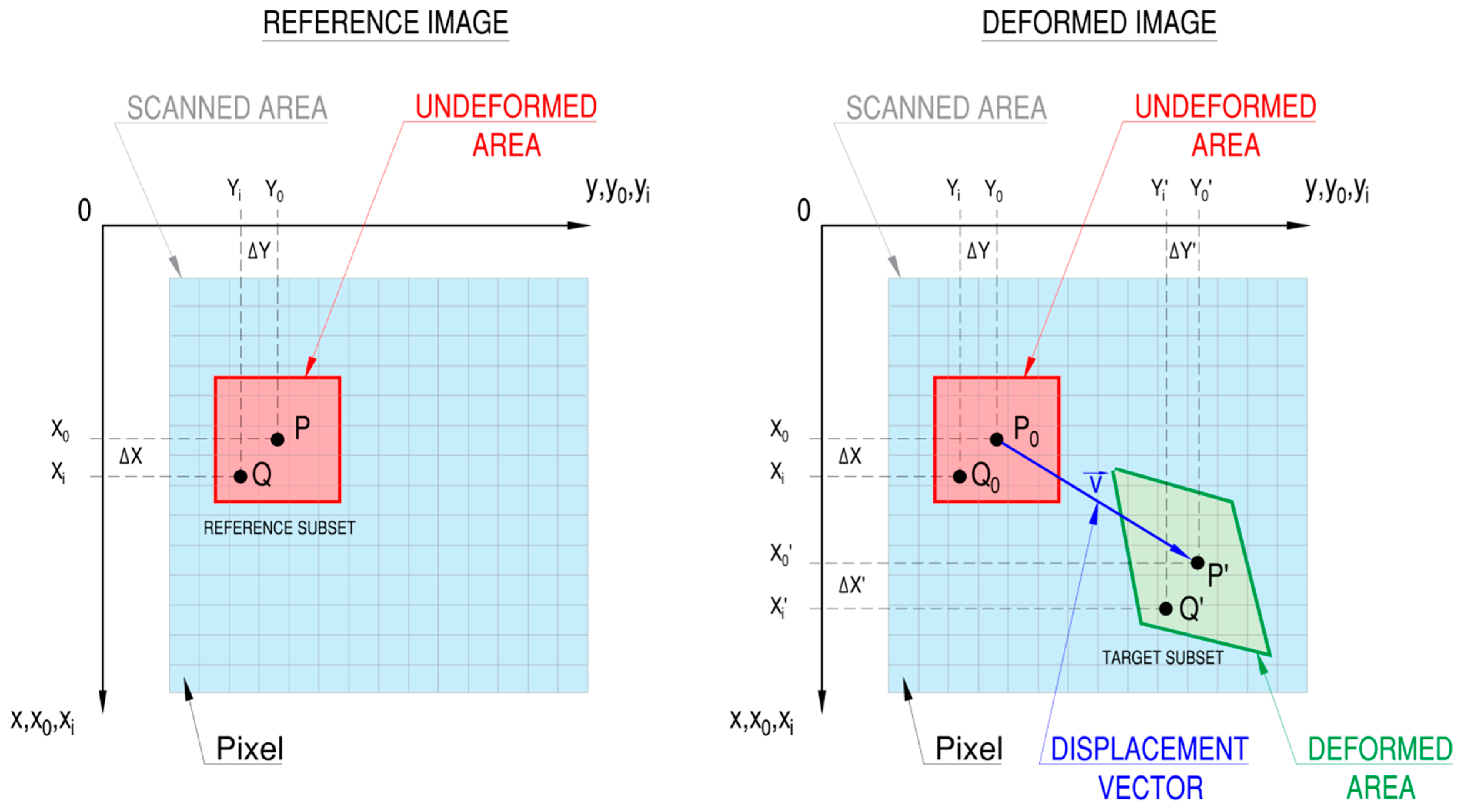
2.1. 2D DIC Background

| Type | Name | Definition | |
|---|---|---|---|
| Cross-correlation criteria | Cross-correlation | (5) | |
| Normalized cross-correlation | (6) | ||
| (7) | |||
| Zero-normalized cross-correlation | (8) | ||
| (9) | |||
| (10) | |||
| (11) | |||
| Sum-squared difference correlation criteria | Sum of squared differences | (12) | |
| Normalized sum of squared differences | (13) | ||
| Zero-normalized sum of squared differences | (14) |
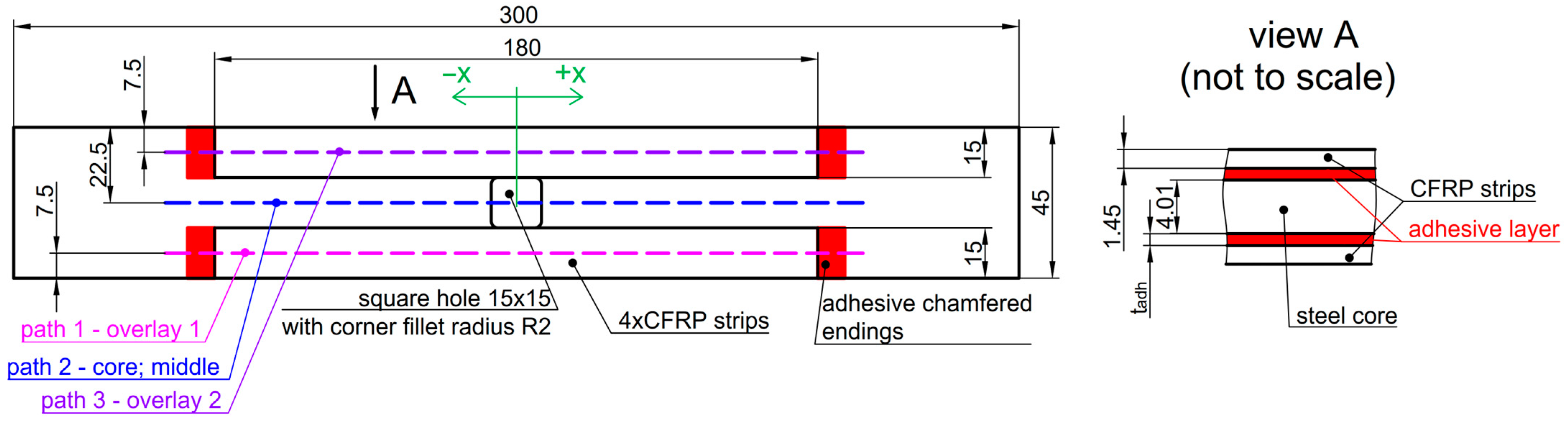
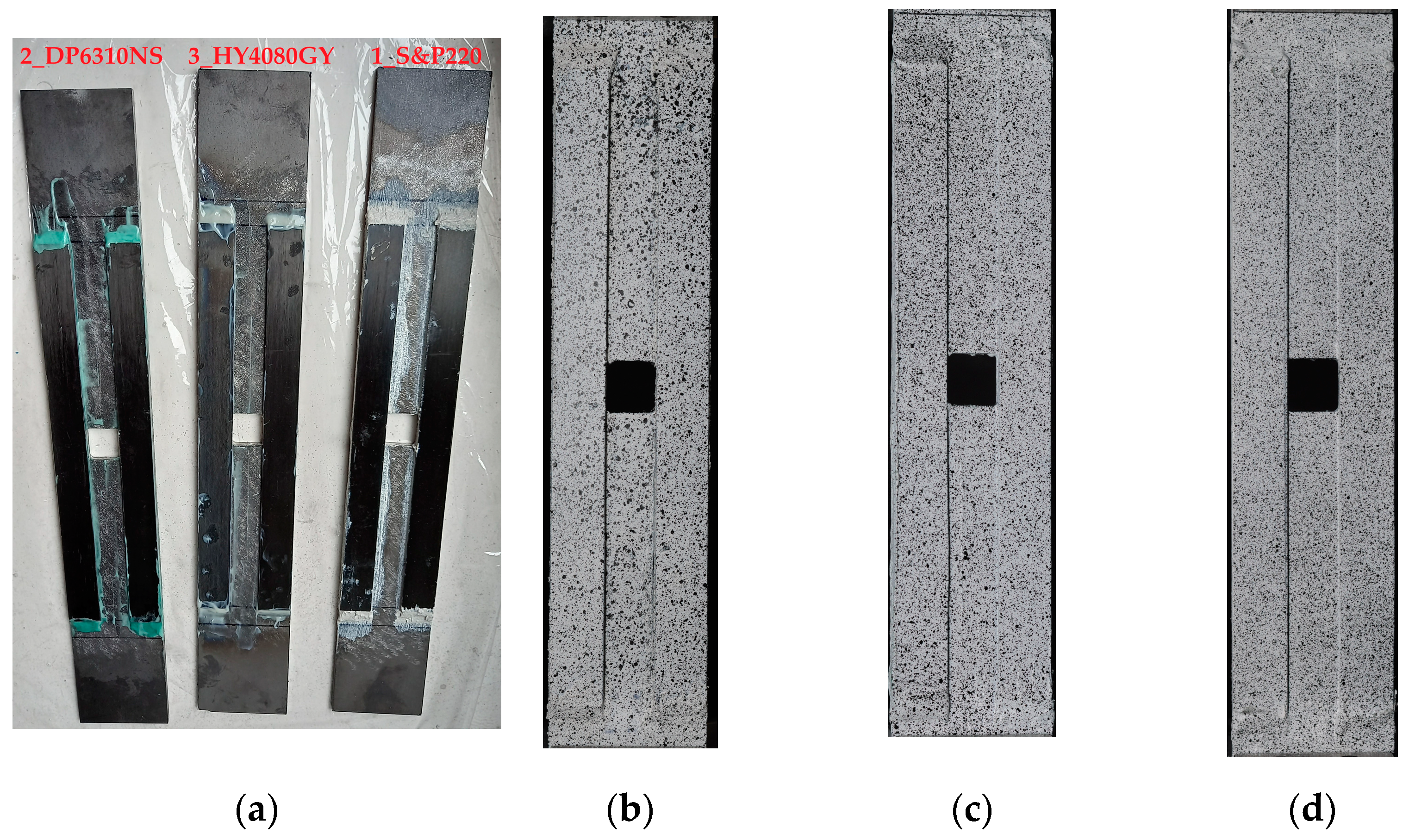
2.2. Materials and Samples
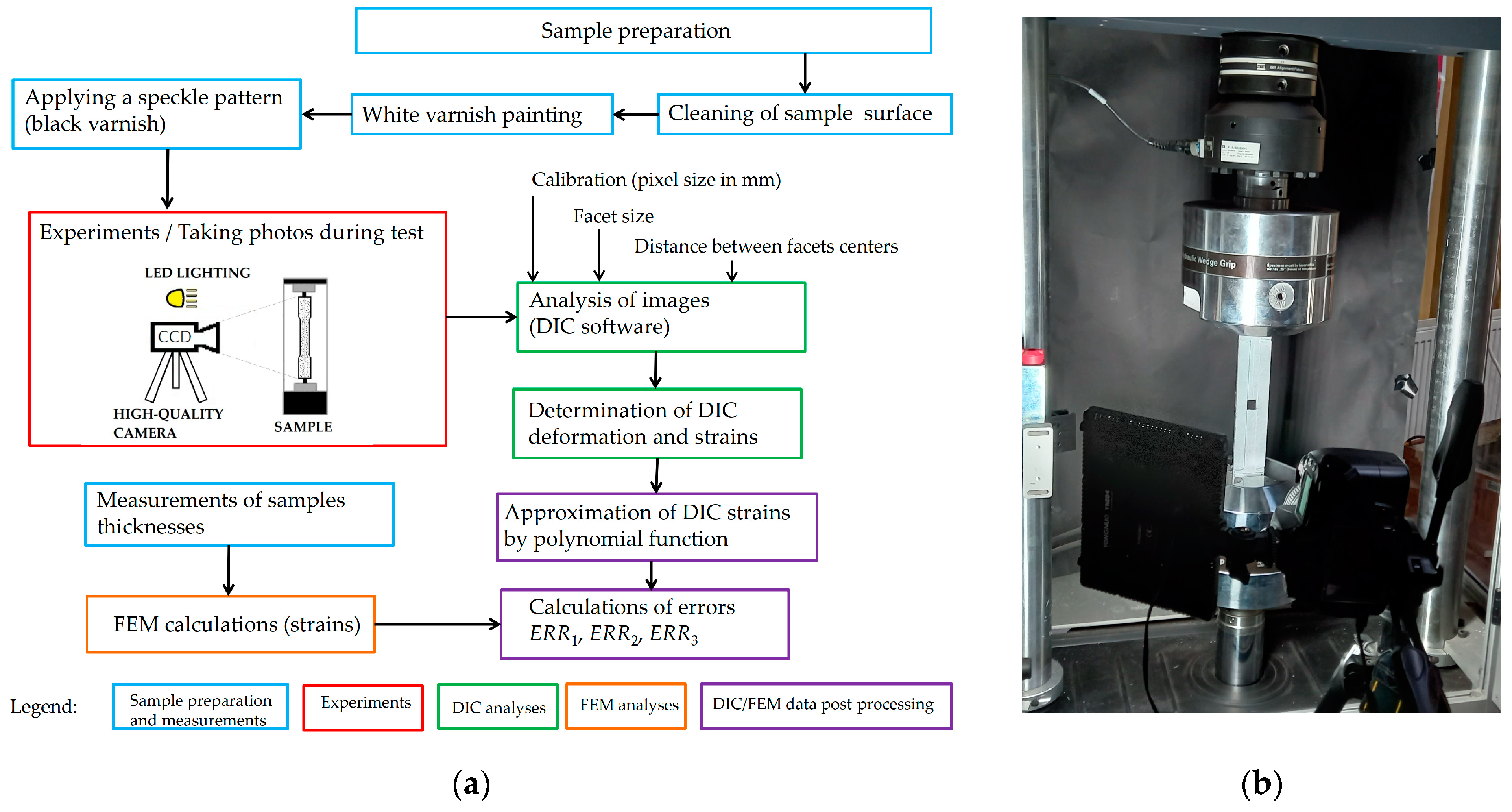
2.3. DIC System
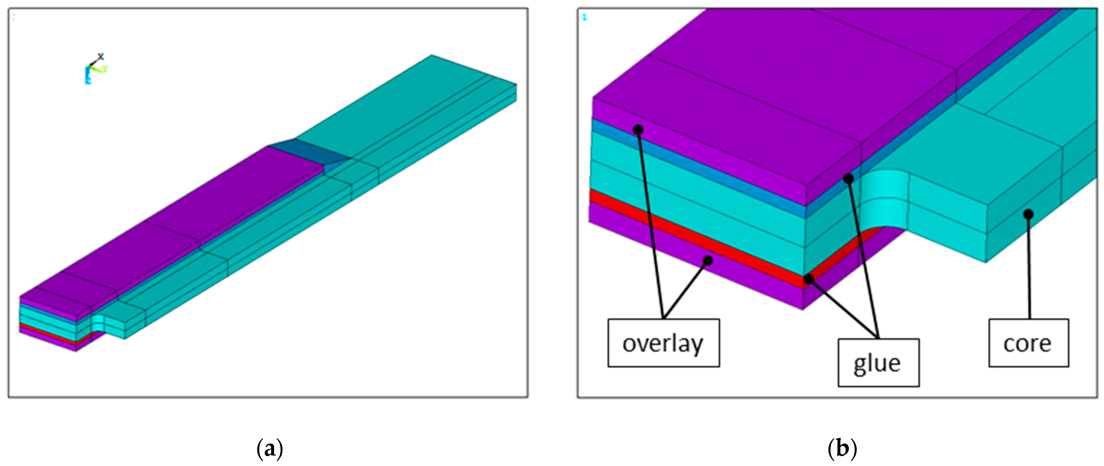
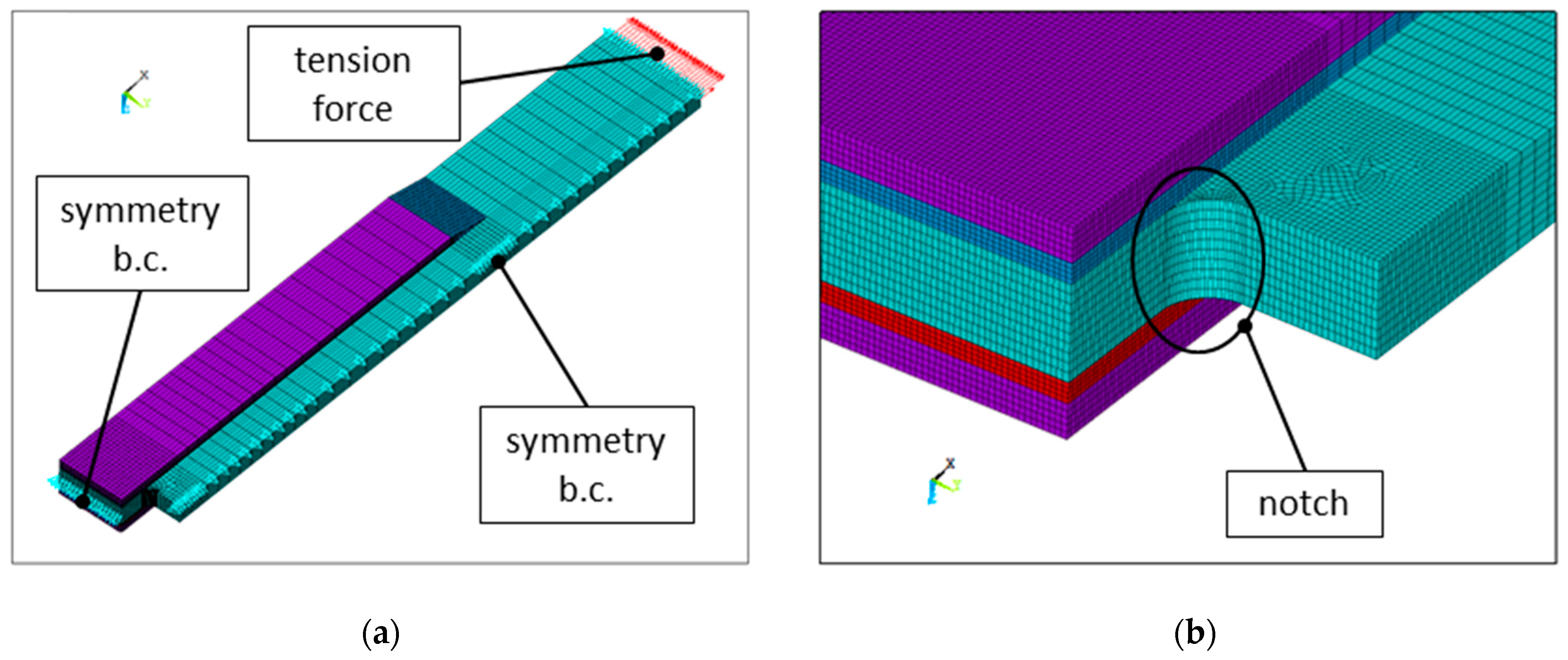
2.4. FEM Model
2.5. Proposed Methodology for Evaluation of DIC Accuracy
3. Results
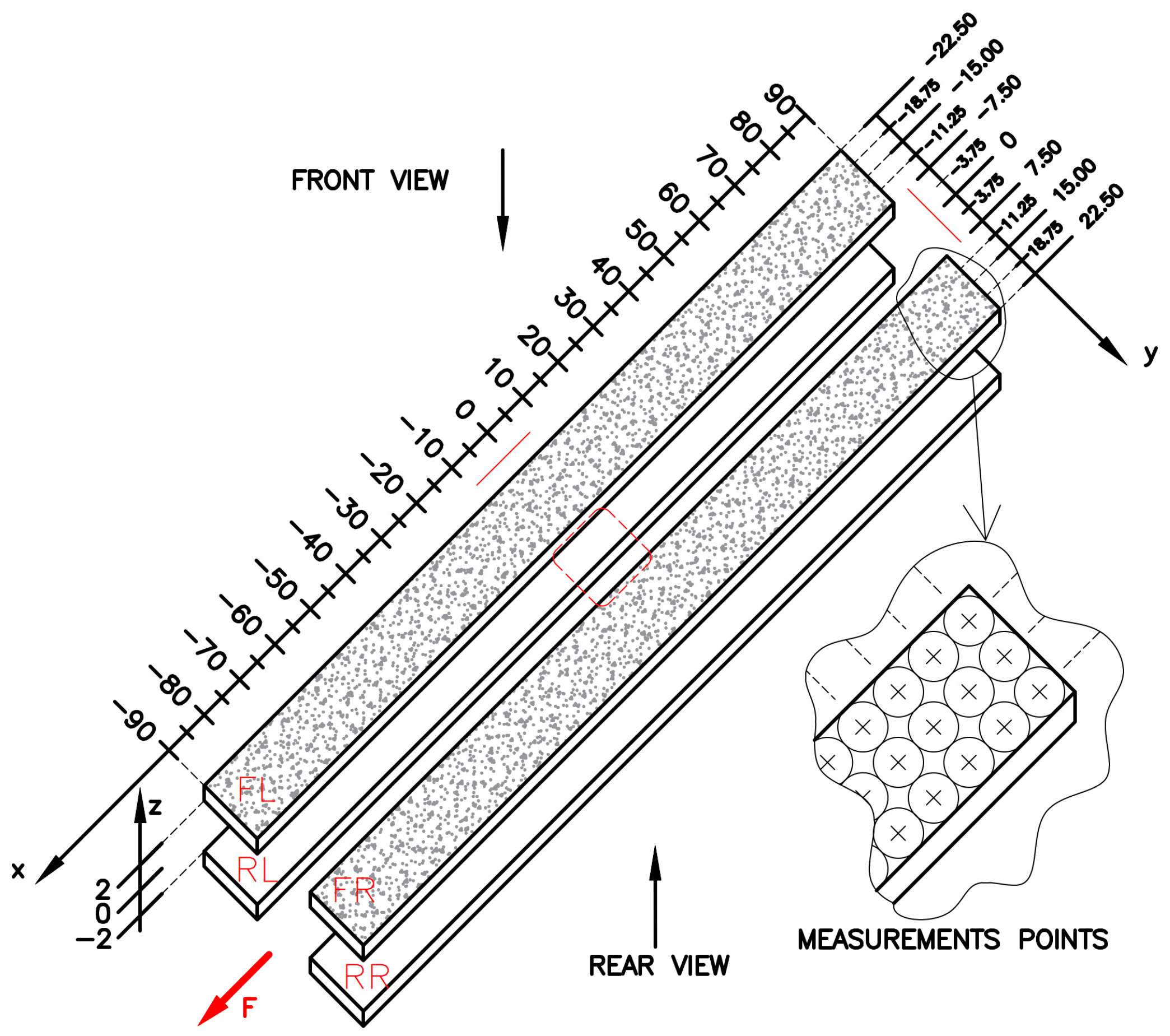
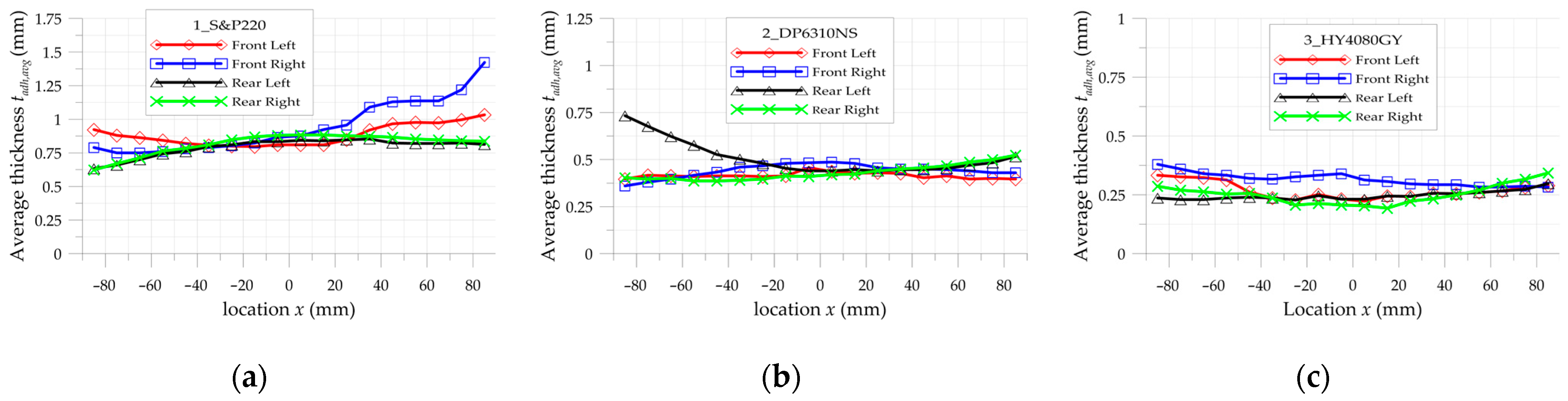
3.1. Measurements of Real Adhesive Thickness
3.2. Validation of the FEM Model
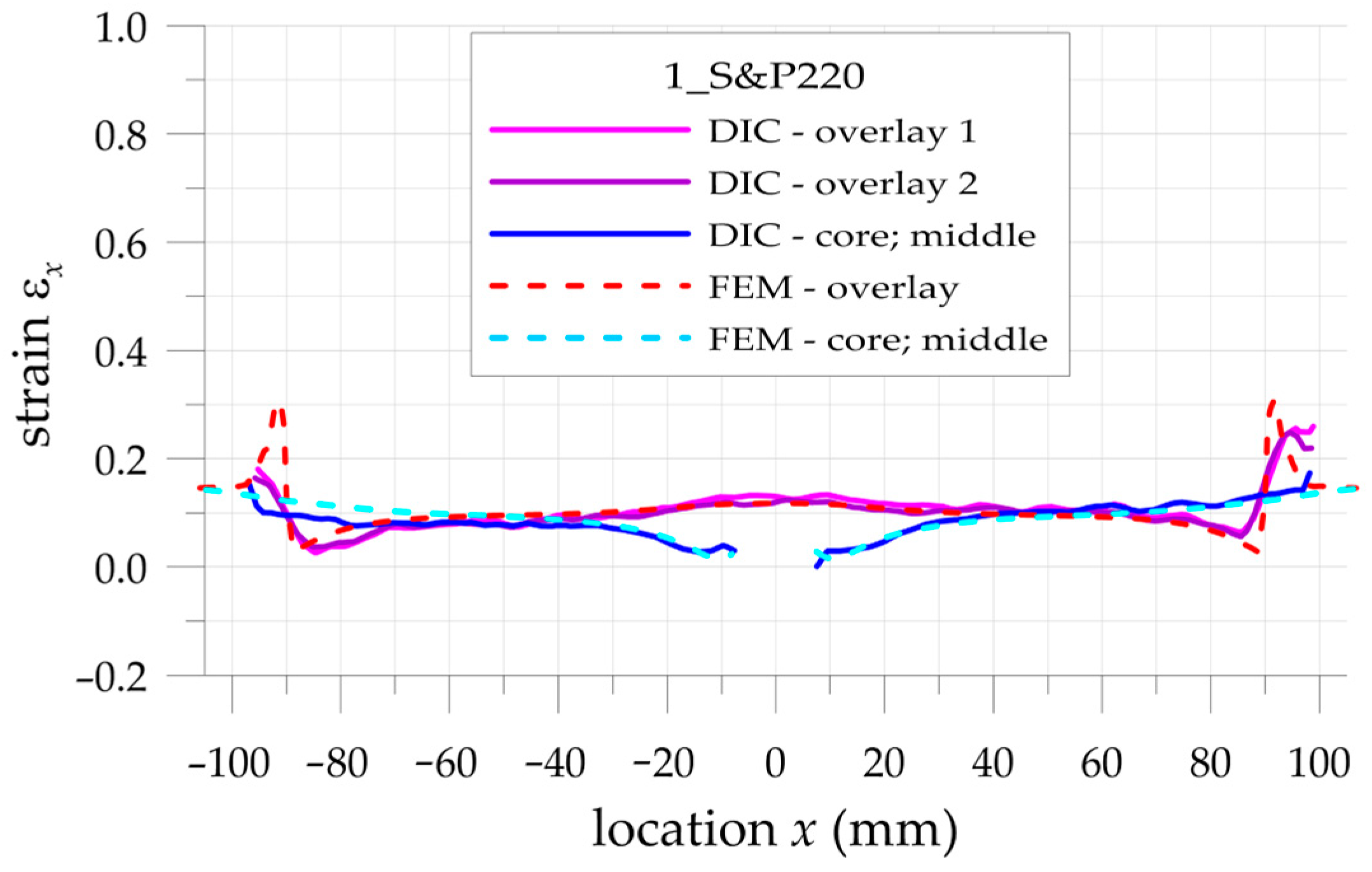
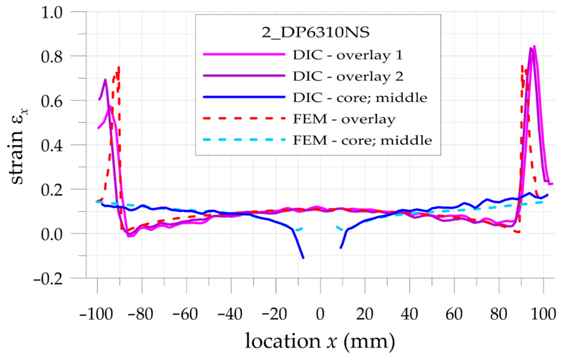
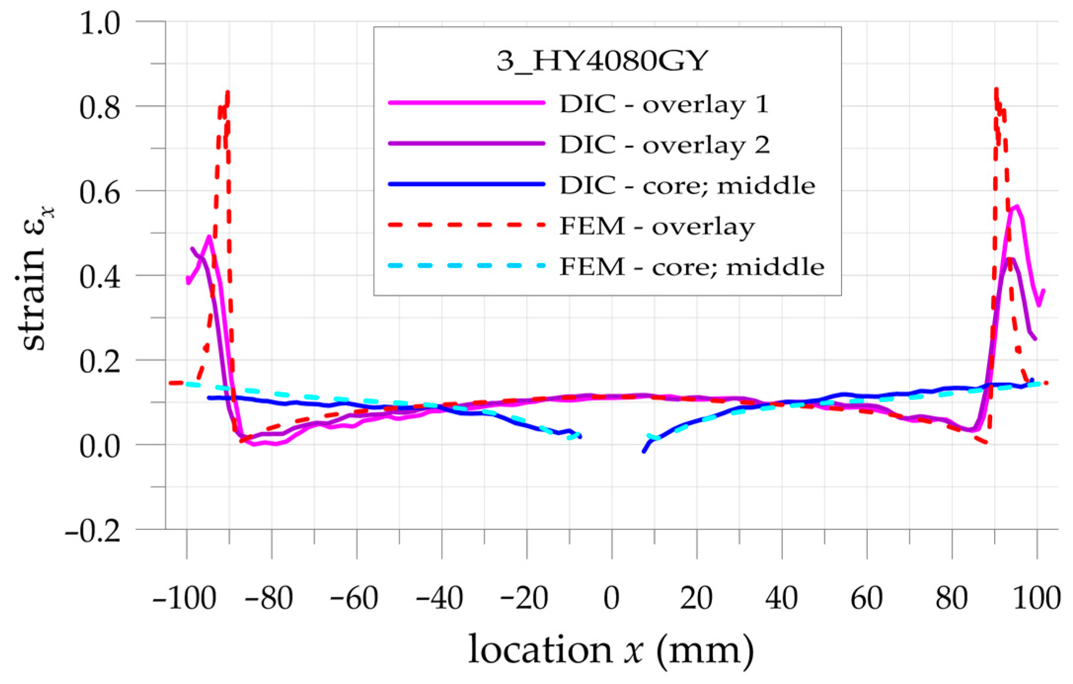
3.3. Full-Scale Surface Strain Study
- change of the materials (stiff CFRP overlays/soft adhesive/stiff steel core).
- inclination of the adhesive chamfered endings with respect to the CFRP overlays and steel core.
- the rough and folded surface of the adhesive chamfered endings.
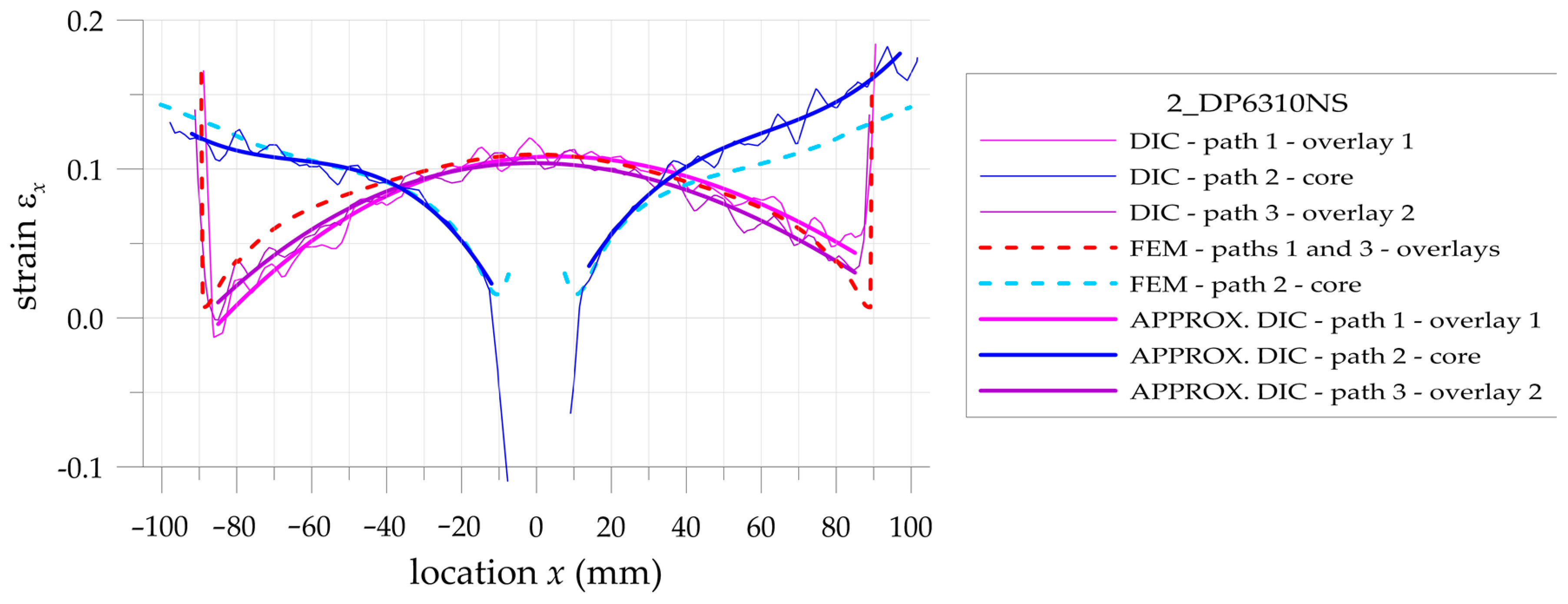
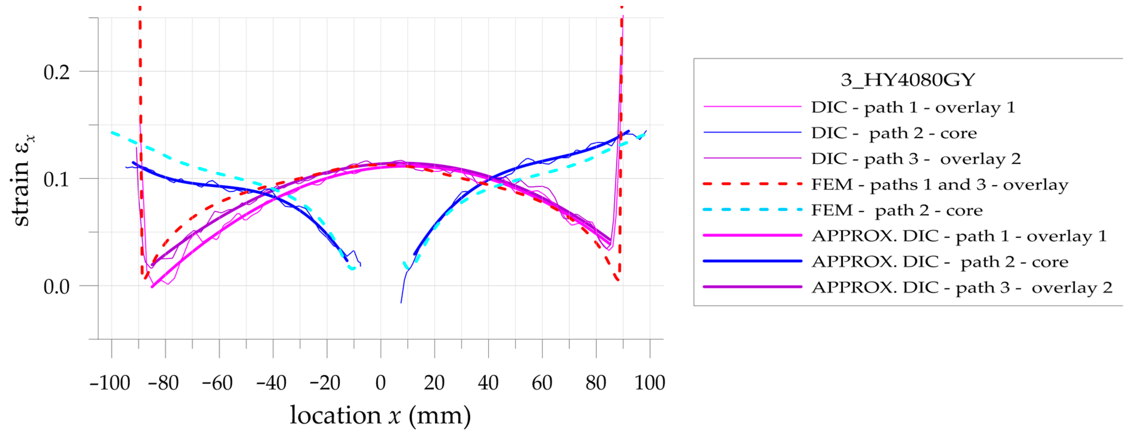
3.4. Comparison of DIC and FEM Results
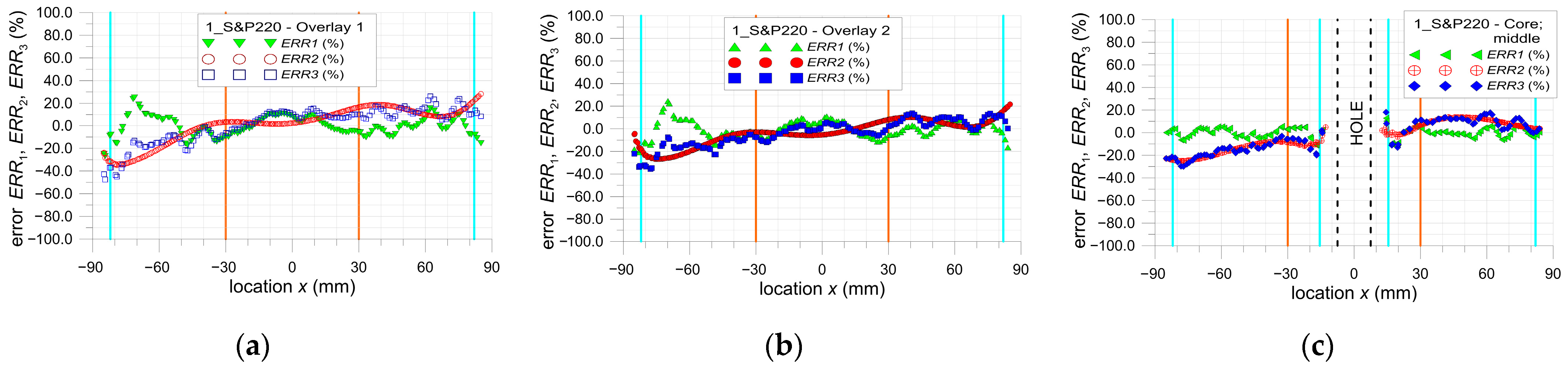
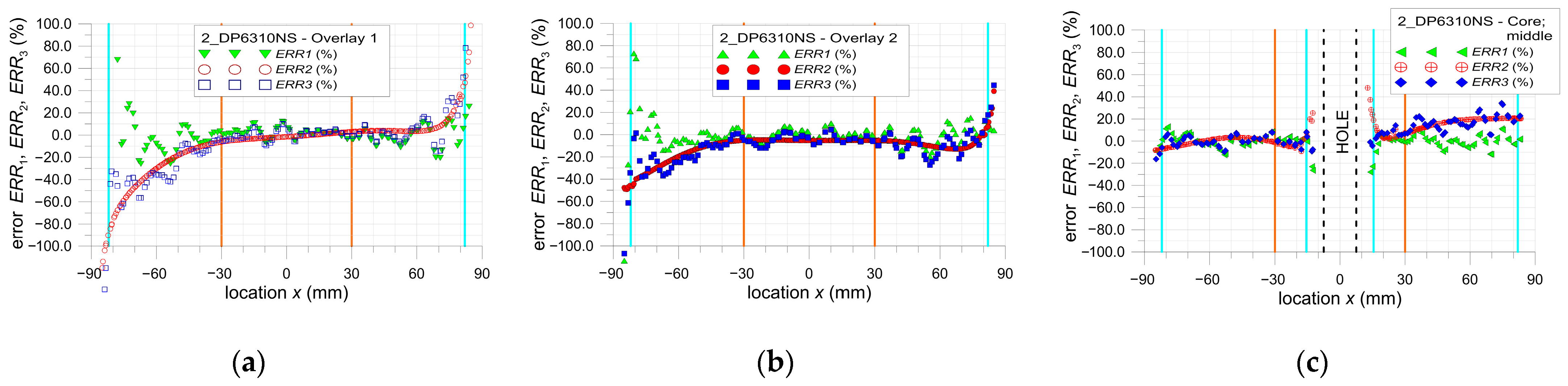
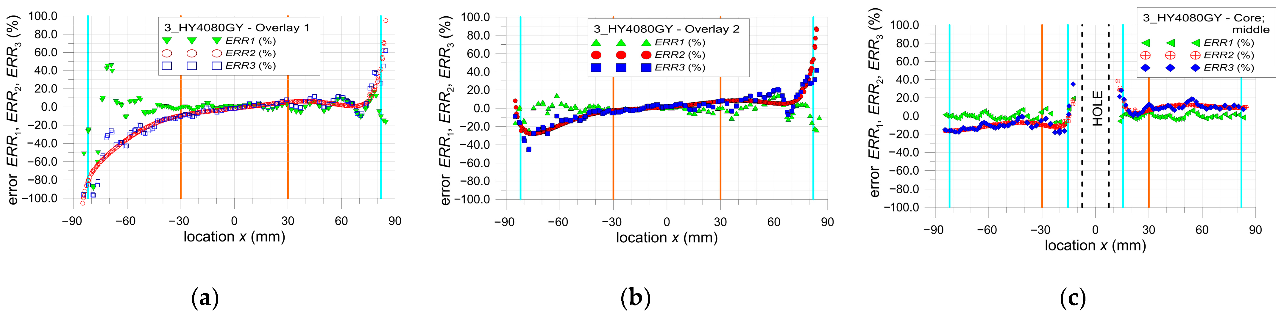
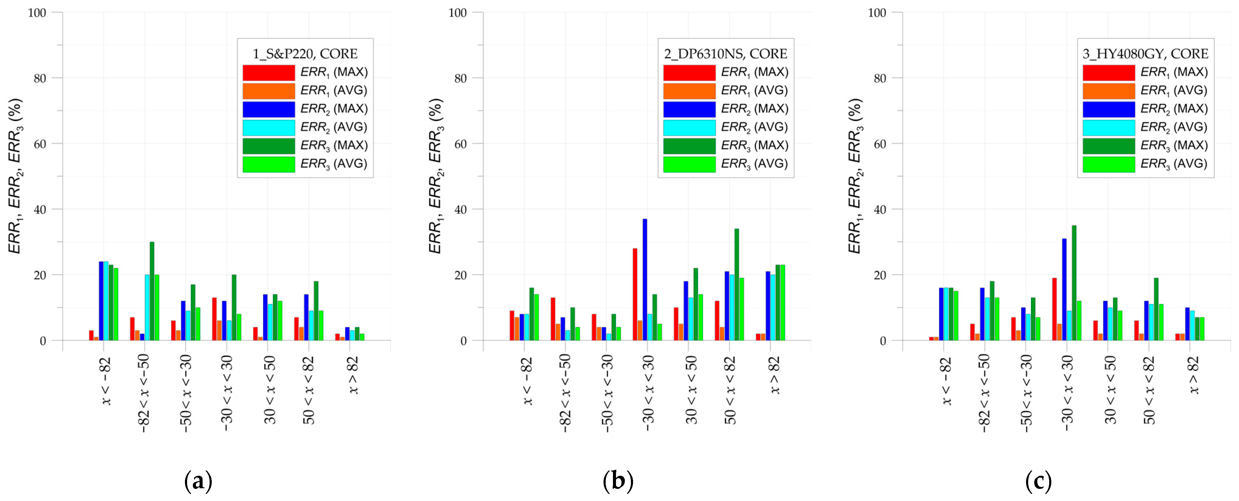
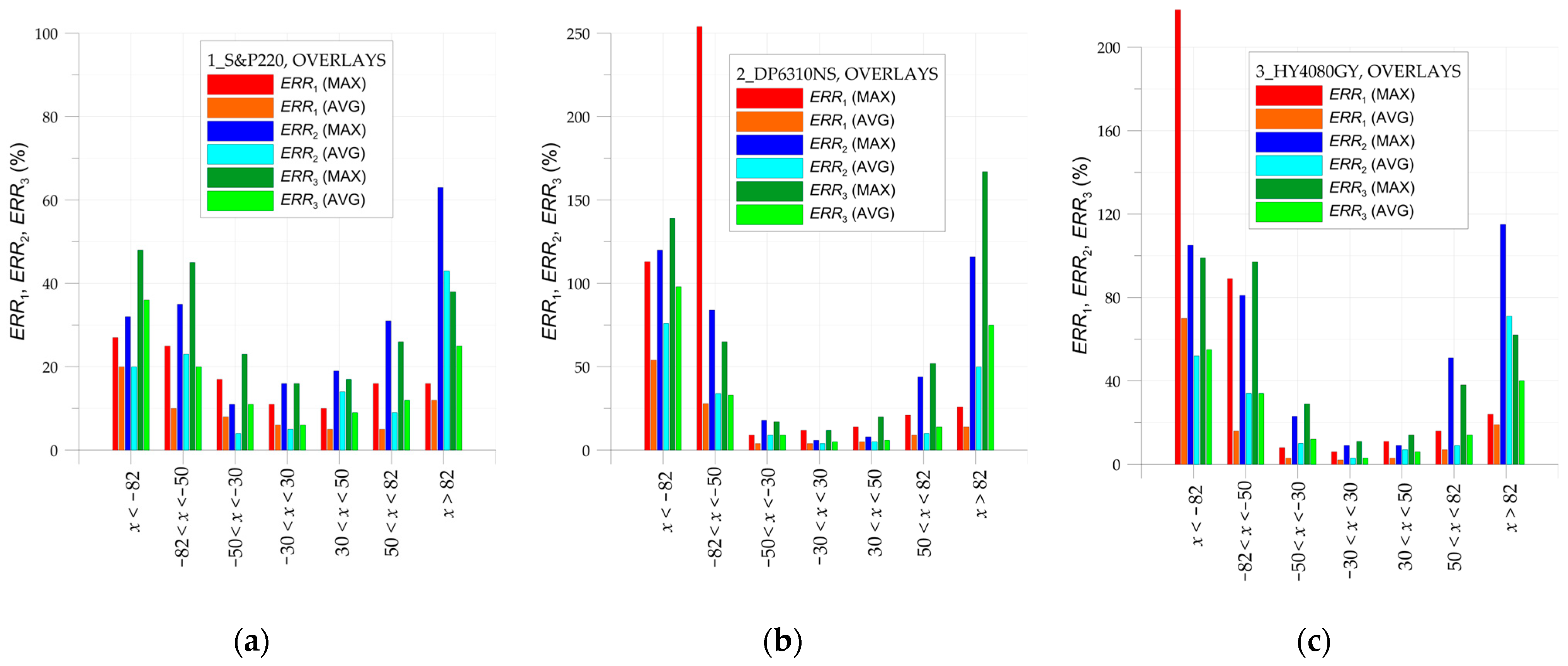
3.5. Accuracy and Error Analyses
4. Discussion
- the mechanism of the load transfer from the steel core to the overlays, which may have a very complex nature.
- influence of the shape of adhesive-chamfered endings on the final results.
- variable adhesive thickness, which is not taken into account in the FE model.
5. Conclusions
- DIC can be successfully applied for the measurements of elastic strains in hybrid steel/adhesive/composite samples, including elastic strains in the steel core.
- The error of strains evaluated by means of the DIC method can be assessed by the analysis of the amplitudes of the strain fluctuations.
- The application of the third-level polynomial approximation function allows for the reduction of the fluctuation of strains, which results in a more smoother distribution of surface strains and leads to a more accurate solution with respect to FEM results.
- In the central parts of the samples ( the errors ERR2 and ERR3 do not exceed 30% (the maximal absolute errors) and 15% (the average absolute errors) for overlays, and 35% (the maximal absolute errors) and 14% (the average absolute errors) for steel core. For a narrowed analysis area ( and overlays, the errors ERR2 and ERR3 are reduced to 16% (the maximal absolute errors) and 6% (the average absolute errors). The values of the above-issued errors are fully acceptable for the measurements of strains in engineering structures.
- The largest differences between DIC and FEM results are observed on the overlays in the vicinities of the rounded corners of the rectangular holes. The observed strain concentrations in all samples in DIC analyses at such points are not noticed in FEM analyses.
Author Contributions
Funding
Institutional Review Board Statement
Informed Consent Statement
Data Availability Statement
Acknowledgments
Conflicts of Interest
References
- Lee, S.H. A CAD–CAE integration approach using feature-based multi-resolution and multi-abstraction modelling techniques. Comput. Aided Design 2005, 371, 941–955. [Google Scholar] [CrossRef]
- Kärger, L.; Bernath, A.; Fritz, F.; Galkin, S.; Magagnato, D.; Oeckerath, A.; Schön, A.; Henning, F. Development and validation of a CAE chain for unidirectional fibre reinforced composite components. Compos. Struct. 2015, 132, 350–358. [Google Scholar] [CrossRef]
- Cuesta, C.; Luque, P.; Mantaras, D.A. A methodology to improve simulation of multibody systems using estimation techniques. Automatika 2022, 63, 16–25. [Google Scholar] [CrossRef]
- Freddi, A.; Olmi, G.; Cristofolini, L. Experimental Stress Analysis for Materials and Structures. Stress Analysis Models for Developing Design Methodologies, 1st ed.; Springer: Berlin/Heidelberg, Germany, 2015. [Google Scholar] [CrossRef]
- Phillips, J.W. (Ed.) TAM 326—Experimental Stress Analysis; University of Illinois: Champaign, IL, USA, 2000; pp. 1–62. [Google Scholar]
- Lee, Y.L.; Pan, J.; Hathaway, R.B.; Barkey, M.E. Fatigue Testing and Analysis: Theory and Practice; Elsevier Butterworth-Heinemann: Burlington, VT, USA, 2005. [Google Scholar] [CrossRef]
- Romanowicz, P.J.; Szybiński, B. Determination of Optimal Flat-End Head Geometries for Pressure Vessels Based on Numerical and Experimental Approaches. Materials 2021, 14, 2520. [Google Scholar] [CrossRef] [PubMed]
- Szybiński, B.; Romanowicz, P.; Zieliński, A.P. Numerical and experimental analysis of stress and strains in flat ends of high-pressure vessels. Key Eng. Mater. 2011, 490, 226–236. [Google Scholar] [CrossRef]
- Giurgiutiu, V. Structural Health Monitoring with Piezoelectric Wafer Active Sensors, 2nd ed.; Elsevier: Kidlington, UK, 2014. [Google Scholar]
- Guo, H.; Xiao, G.; Mrad, N.; Yao, J. Fiber Optic Sensors for Structural Health Monitoring of Air Platforms. Sensors 2011, 11, 3687–3705. [Google Scholar] [CrossRef] [PubMed]
- García, I.; Zubia, J.; Durana, G.; Aldabaldetreku, G.; Illarramendi, M.A.; Villatoro, J. Optical Fiber Sensors for Aircraft Structural Health Monitoring. Sensors 2015, 15, 15494–15519. [Google Scholar] [CrossRef] [PubMed]
- Wild, G.; Hinckley, S. Acousto-Ultrasonic optical fiber sensors: Overview and state-of-the-art. IEEE Sens. J. 2008, 8, 1184–1193. [Google Scholar] [CrossRef]
- Yoshino, T.; Kurosawa, K.; Itoh, K.; Ose, T. Fiber-optic Fabry-Perot interferometer and its sensor applications. IEEE J. Quant. Elect. 1982, 4, 626–665. [Google Scholar]
- Barski, M.; Kędziora, P.; Muc, A.; Romanowicz, P. Structural health monitoring (shm) methods in machine design and operation. Arch. Mech. Eng. 2014, 61, 653–677. [Google Scholar] [CrossRef]
- Peters, W.H.; Ranson, W.F. Digital imaging techniques in experimental stress analysis. Opt. Eng. 1982, 21, 427–432. [Google Scholar] [CrossRef]
- Peters, W.H.; Ranson, W.F.; Sutton, M.A. Applications of digital image correlation methods to rigid body mechanics. Opt. Eng. 1983, 22, 738–742. [Google Scholar] [CrossRef]
- Sutton, M.A.; Wolters, W.J. Determination of displacement using an improved digital image correlation method. Image Vis. Comput. 1983, 1, 133–139. [Google Scholar] [CrossRef]
- Pan, B.; Qian, K.; Xie, H.; Asundi, A. Two-dimensional digital image correlation for in-plane displacement and strain measurement: A review. Meas. Sci. Technol. 2009, 20, 062001. [Google Scholar] [CrossRef]
- Janeliukstis, R.; Chen, X. Review of digital image correlation application to large-scale composite structures testing. Composite Structures 2021, 271, 113143. [Google Scholar] [CrossRef]
- Pan, B. Digital image correlation for surface deformation measurement: Historical developments, recent advances and future goals. Meas. Sci. Technol. 2018, 29, 082001. [Google Scholar] [CrossRef]
- Sirkis, J.S.; Lim, T.J. Displacement and strain-measurement with automated grid methods. In Experimental Mechanics; Springer Nature Switzerland AG.: Cham, Switzerland, 1991; Volume 31, pp. 382–388. ISSN 0014-4851. [Google Scholar]
- Patorski, K. Moiré methods in interferometry. Opt. Lasers Eng. 1988, 8, 147–170. [Google Scholar] [CrossRef]
- Gansan, A.R. Holographic and Laser Speckle Methods in Non-Destructive Testing. In Proceedings of the National Seminar & Exhibition on Non-Destructive Evaluation NDE 2009, Tiruchirapalli, India, 10–12 December 2009. [Google Scholar]
- Pan, B. Bias error reduction of digital image correlation using Gaussian pre-filtering. Opt. Lasers Eng. 2013, 51, 1161–1167. [Google Scholar] [CrossRef]
- Chu, T.C.; Ranson, M.A.; Sutton, M.A.; Peters, W.H. Application of digital-image-correlation techniques to experimental mechanics. In Experimental Mechanics; Springer Nature Switzerland AG.: Cham, Switzerland, 1985; Volume 25, pp. 232–244. ISSN 0014-4851. [Google Scholar]
- Romanowicz, P. Experimental and numerical estimation of the damage level in multilayered composite plates. Mater. Und Werkst. 2018, 49, 591–605. [Google Scholar] [CrossRef]
- Muc, A.; Chwał, M.; Romanowicz, P.; Stawiarski, A. Fatigue-Damage Evolution of Notched Composite Multilayered Structures under Tensile Loads. J. Compos. Sci. 2018, 2, 27. [Google Scholar] [CrossRef]
- Visser, C.-H.; Venter, G.; Neaves, M. A Strain-Gauge-Based Method for the Compensation of Out-of-Plane Motions in 2D Digital Image Correlation. Math. Comput. Appl. 2023, 28, 40. [Google Scholar] [CrossRef]
- Haddadi, H.; Belhabib, S. Use of rigid-body motion for the investigation and estimation of the measurement errors related to digital image correlation technique. Opt. Lasers Eng. 2008, 46, 185–196. [Google Scholar] [CrossRef]
- Cui, H.; Zeng, Z.; Zhang, H.; Yang, F. Reducing the systematic error of DIC using gradient filtering. Measurement 2023, 207, 112366. [Google Scholar] [CrossRef]
- Bornert, M.; Bremand, F.; Doumalin, P.; Dupre, J.C.; Fazzini, M.; Grediac, M.; Hild, F.; Mistou, S.; Molimard, J.; Orteu, J.J.; et al. Assessment of Digital Image Correlation Measurement Errors: Methodology and Results. Exp. Mech. 2009, 49, 353–370. [Google Scholar] [CrossRef]
- Wang, L.; Liu, G.; Xing, T.; Zhu, H.; Ma, S. Boundary Deformation Measurement by Mesh-Based Digital Image Correlation Method. Appl. Sci. 2020, 11, 53. [Google Scholar] [CrossRef]
- Wang, B.; Pan, B. Subset-based local vs. finite element-based global digital image correlation: A comparison study. Theor. Appl. Mech. Lett. 2016, 6, 200–208. [Google Scholar] [CrossRef]
- Kosmann, J.; Völkerink, O.; Schollerer, M.J.; Holzhüter, D.; Hühne, C. Digital image correlation strain measurement of thick adherend shear test specimen joined with an epoxy film adhesive. Int. J. Adhes. Adhes. 2019, 90, 32–37. [Google Scholar] [CrossRef]
- Srilakshmi, R.; Ramji, M. Experimental investigation of adhesively bonded patch repair of an inclined center cracked panel using DIC. J. Reinf. Plast. Compos. 2014, 33, 1130–1147. [Google Scholar] [CrossRef]
- Kashfuddoja, M.; Ramji, M. Critical analysis of adhesive layer behavior in patch-repaired carbon fiber-reinforced polymer panel involving digital image correlation. J. Compos. Mater. 2015, 49, 2015–2028. [Google Scholar] [CrossRef]
- Seon, G.; Makeev, A.; Schaefer, J.D.; Justusson, B. Measurement of Interlaminar Tensile Strength and Elastic Properties of Composites Using Open-Hole Compression Testing and Digital Image Correlation. Appl. Sci. 2019, 9, 2647. [Google Scholar] [CrossRef]
- Peng, J.; Zhou, P.; Wang, Y.; Dai, Q.; Knowles, D.; Mostafavi, M. Stress Triaxiality and Lode Angle Parameter Characterization of Flat Metal Specimen with Inclined Notch. Metals 2021, 11, 1627. [Google Scholar] [CrossRef]
- Lemmen, H.J.K.; Alderliesten, R.C.; Benedictus, R.; Hofstede, J.C.J.; Rodi, R. The power of Digital Image Correlation for detailed elastic-plastic strain measurements. In Proceedings of the Engineering Mechanics, Structures, Engineering Geology conference (EMESEG ‘08), Heraklion, Greece, 22–24 July 2008. [Google Scholar]
- Aidi, B.; Case, S.W. Experimental and numerical monitoring of strain gradients in notched composites under tension loading. In Proceedings of the 56th AIAA/ASCE/AHS/ASC Structures, Structural Dynamics, and Materials Conference, Kissimmee, FL, USA, 5–9 January 2015; American Institute of Aeronautics and Astronautics: Reston, WV, USA, 2015. [Google Scholar] [CrossRef]
- Romanowicz, P.J.; Szybiński, B.; Wygoda, M. Application of DIC Method in the Analysis of Stress Concentration and Plastic Zone Development Problems. Materials 2020, 13, 3460. [Google Scholar] [CrossRef] [PubMed]
- Romanowicz, P.J.; Szybiński, B.; Wygoda, M. Preliminary Experimental and Numerical Study of Metal Element with Notches Reinforced by Composite Materials. J. Compos. Sci. 2021, 5, 134. [Google Scholar] [CrossRef]
- Romanowicz, P.J.; Szybiński, B.; Wygoda, M. Static and Fatigue Behaviour of Double-Lap Adhesive Joints and Notched Metal Samples Reinforced by Composite Overlays. Materials 2022, 15, 3233. [Google Scholar] [CrossRef] [PubMed]
- Romanowicz, P.J.; Szybiński, B.; Wygoda, M. Fatigue performance of open-hole structural elements reinforced by CFRP overlays. Int. J. Adhes. Adhes. 2024, 130, 103606. [Google Scholar] [CrossRef]
- Peng-Da, L.; Zhao, Y.; Tao, Z.; Jiang, C. Nonuniformity in stress transfer across FRP width of FRP-concrete interface. Eng. Struct. 2024, 312, 118236. [Google Scholar]
- Jaing, C. Strength enhancement due to FRP confinement for coarse aggregate-free concretes. Eng. Struct. 2023, 277, 115370. [Google Scholar] [CrossRef]
- Cao, J.; Du, J.; Fan, Q.; Yang, J.; Bao, C.; Liu, Y. Reinforcement for earthquake-damaged glued-laminated timber knee-braced frames with self-tapping screws and CFRP fabric. Eng. Struct. 2024, 306, 117787. [Google Scholar] [CrossRef]
- Lu, H.; Cary, P.D. Deformation measurement by digital image correlation: Implementation of a second-order displacement gradient. In Experimental Mechanics; Springer: Cham, Switzerland, 2000; Volume 40, pp. 393–400. ISSN 0014-4851. [Google Scholar]
- Schreier, H.W.; Sutton, M.A. Systematic errors in digital image correlation due to undermatched subset shape function. Exp. Mech. 2002, 42, 303–310. [Google Scholar] [CrossRef]
- GOM Software 2018 Hotfix 1. Available online: www.gom.com (accessed on 26 September 2018).
- ANSYS. Campus Release 2022 R2 July 2022; ANSYS, Inc.: Canonsburg, PA, USA, 2022. [Google Scholar]
- Shahmardani, M.; Ståhle, P.; Islam, M.S.; Kao-Walter, S. Numerical Simulation of Buckling and Post-Buckling Behavior of a Central Notched Thin Aluminum Foil with Nonlinearity in Consideration. Metals 2020, 10, 582. [Google Scholar] [CrossRef]
- Barski, M.; Stawiarski, A.; Romanowicz, P.J.; Szybiński, B. Local elasto-plastic buckling of isotropic plates with cutouts under tension loading conditions. Int. J. Mech. 2021, 15, 69–87. [Google Scholar] [CrossRef]
- Romanowicz, P.; Muc, A. Estimation of Notched Composite Plates Fatigue Life Using Residual Strength Model Calibrated by Step-Wise Tests. Materials 2018, 11, 2180. [Google Scholar] [CrossRef] [PubMed]


| Chemical Composition (in % Weight) | Minimal Yield Stress | Ultimate Tensile Strength (UTS) | ||||||||
|---|---|---|---|---|---|---|---|---|---|---|
| C | Mn | Si | Al | Cu | Cr | S | P | Fe | ||
| 0.15 | 1.33 | 0.13 | 0.04 | 0.02 | 0.02 | 0.04 | 0.01 | Res. | 427 MPa | 528 MPa |
| Material | Type | E1 (GPa) | E2, E3 (GPa) | G12, G23 (GPa) | G31 (GPa) | ν1, ν2 | ν3 | UTS (MPa) |
|---|---|---|---|---|---|---|---|---|
| S&P C-Laminate 150/2000 | CFRP | 165 | 10 | 5 | 0.5 | 0.3 | 0.03 | 2800 |
| S&P Resin 220 | Adhesive | 7 | - | - | - | - | - | 14 |
| DP 6310 NS | 0.59 | - | - | - | - | - | 18.6 | |
| HY 4080 GY | 0.355 | - | - | - | - | - | 11.3 |
| Designation | Adhesive | Average Adhesive Thickness (mm) |
|---|---|---|
| 1_S&P220 | S&P Resin 220 | 0.86 (SD: 0.14 mm) |
| 2_DP6310NS | DP 6310 NS | 0.62 (SD: 0.18 mm) |
| 3_HY4080GY | HY 4080 GY | 0.27 (SD: 0.06 mm) |
| Designation | Maximal Surface Strain (%) | |||
|---|---|---|---|---|
| DIC (1) | FEM | DIC | FEM | |
| 1_S&P220 | 0.18/0.16 | 0.31 | 0.26/0.25 | 0.31 |
| 2_DP6310NS | 0.57/0.69 | 0.76 | 0.84/0.83 | 0.76 |
| 3_HY4080GY | 0.49/0.44 | 0.85 | 0.56/0.44 | 0.85 |
| Location x (mm) | Maximal Surface Strain (%) (1) | ||||||||
|---|---|---|---|---|---|---|---|---|---|
| 1_S&P220 | 2_DP6310NS | 3_HY4080GY | |||||||
| DIC | DIC APPR. | FEM | DIC | DIC APPR. | FEM | DIC | DIC APPR. | FEM | |
| −80 | 0.038/0.045 | 0.044/0.051 | 0.066 | 0.025/0.036 | 0.008/0.021 | 0.038 | 0.005/0.025 | 0.010/0.029 | 0.038 |
| −60 | 0.079/0.080 | 0.073/0.074 | 0.093 | 0.048/0.056 | 0.052/0.059 | 0.074 | 0.044/0.068 | 0.050/0.063 | 0.078 |
| −40 | 0.095/0.089 | 0.096/0.092 | 0.097 | 0.076/0.080 | 0.082/0.085 | 0.091 | 0.079/0.090 | 0.080/0.088 | 0.094 |
| −20 | 0.110/0.104 | 0.111/0.104 | 0.109 | 0.101/0.092 | 0.100/0.100 | 0.105 | 0.100/0.104 | 0.100/0.106 | 0.107 |
| 0 | 0.129/0.118 | 0.120/0.111 | 0.118 | 0.115/0.107 | 0.108/0.104 | 0.110 | 0.110/0.114 | 0.110/0.114 | 0.112 |
| 20 | 0.117/0.105 | 0.121/0.112 | 0.109 | 0.108/0.100 | 0.106/0.099 | 0.105 | 0.106/0.112 | 0.110/1.112 | 0.107 |
| 40 | 0.112/0.110 | 0.115/0.107 | 0.097 | 0.087/0.080 | 0.095/0.86 | 0.091 | 0.100/0.097 | 0.099/0.101 | 0.094 |
| 60 | 0.113/0.101 | 0.102/0.095 | 0.093 | 0.079/0.065 | 0.077/0.065 | 0.074 | 0.086/0.093 | 0.079/0.082 | 0.078 |
| 80 | 0.075/0.077 | 0.082/0.078 | 0.066 | 0.048/0.041 | 0.051/0.038 | 0.038 | 0.055/0.048 | 0.048/0.052 | 0.038 |
| Location x (mm) | Maximal Surface Strain (%) | ||||||||
|---|---|---|---|---|---|---|---|---|---|
| 1_S&P220 | 2_DP6310NS | 3_HY4080GY | |||||||
| DIC | DIC APPR. | FEM | DIC | DIC APPR. | FEM | DIC | DIC APPR. | FEM | |
| −80 | 0.088 | 0.084 | 0.113 | 0.125 | 0.113 | 0.120 | 0.099 | 0.101 | 0.120 |
| −60 | 0.083 | 0.079 | 0.096 | 0.102 | 0.105 | 0.103 | 0.093 | 0.092 | 0.103 |
| −40 | 0.076 | 0.079 | 0.086 | 0.091 | 0.091 | 0.089 | 0.089 | 0.083 | 0.090 |
| −20 | 0.045 | 0.047 | 0.052 | 0.054 | 0.052 | 0.054 | 0.045 | 0.048 | 0.054 |
| 20 | 0.047 | 0.052 | 0.052 | 0.059 | 0.057 | 0.054 | 0.055 | 0.058 | 0.054 |
| 40 | 0.098 | 0.097 | 0.086 | 0.102 | 0.102 | 0.089 | 0.101 | 0.100 | 0.090 |
| 60 | 0.112 | 0.108 | 0.096 | 0.116 | 0.124 | 0.103 | 0.114 | 0.116 | 0.103 |
| 80 | 0.112 | 0.116 | 0.113 | 0.141 | 0.145 | 0.120 | 0.134 | 0.132 | 0.120 |
| Investigated Zone (mm) | ||||||||
|---|---|---|---|---|---|---|---|---|
| Maximal Absolute Observed Error/Average Absolute Error (%) | ||||||||
| 1_S&P220 | ERR1 | 27/20 | 25/10 | 17/8 | 11/6 | 10/5 | 16/5 | 16/12 |
| ERR2 | 32/20 | 35/23 | 11/4 | 16/5 | 19/14 | 31/9 | 63/43 | |
| ERR3 | 48/36 | 45/20 | 23/11 | 16/6 | 17/9 | 26/12 | 38/25 | |
| 2_DP6310NS | ERR1 | 113/54 (1) | 254/28 (2) | 9/4 | 12/4 | 14/5 | 21/9 | 26/14 |
| ERR2 | 120/76 | 84/34 | 18/9 | 6/4 | 8/5 | 44/10 (3) | 116/50 | |
| ERR3 | 139/98 | 65/33 | 17/9 | 12/5 | 20/6 | 52/14 (3) | 167/75 | |
| 3_HY4080GY | ERR1 | 218/70 (4) | 89/16 | 8/3 | 6/2 | 11/3 | 16/7 | 24/19 |
| ERR2 | 105/52 (4) | 81/34 | 23/10 | 9/3 | 9/7 | 51/9 | 115/71 | |
| ERR3 | 99/55 | 97/34 | 29/12 | 11/3 | 14/6 | 38/14 | 62/40 | |
| Investigated Zone (mm) | ||||||||
|---|---|---|---|---|---|---|---|---|
| Maximal Absolute Observed Error/Average Absolute Error (%) | ||||||||
| 1_S&P220 | ERR1 | 3/1 | 7/3 | 6/3 | 13/6 | 4/1 | 7/4 | 2/1 |
| ERR2 | 24/24 | 25/20 | 12/9 | 12/6 | 14/11 | 14/9 | 4/3 | |
| ERR3 | 23/22 | 30/20 | 17/10 | 20/8 | 14/12 | 18/9 | 4/2 | |
| 2_DP6310NS | ERR1 | 9/7 | 13/5 | 8/4 | 28/6 (1) | 10/5 | 12/4 | 2/2 |
| ERR2 | 8/8 | 7/3 | 4/2 | 37/8 (1) | 18/13 | 21/20 | 21/20 | |
| ERR3 | 16/14 | 10/4 | 8/4 | 14/5 | 22/14 | 34/19 | 23/23 | |
| 3_HY4080GY | ERR1 | 1/1 | 5/2 | 7/3 | 19/5 | 6/2 | 6/2 | 2/2 |
| ERR2 | 16/16 | 16/13 | 10/8 | 31/9 | 12/10 | 12/11 | 10/9 | |
| ERR3 | 16/15 | 18/13 | 13/7 | 35/12 | 13/9 | 19/11 | 7/7 | |
| ERR2 (AVG) % | ERR3 (AVG) % | ERR2 (MAX) % | ERR3 (MAX) % | (AVG) % | (MAX) % | ||
|---|---|---|---|---|---|---|---|
| 1_S&P220 | Core | 6.9 | 9.3 | 12 | 20 | −25.8 | −40.0 |
| Overlays | 5.5 | 7.3 | 19 | 23 | −24.7 | −17.4 | |
| 2_DP6310NS | Core | 6.5 | 5.9 | 37 | 22 | 10.2 | 68.2 |
| Overlays | 5.0 | 5.4 | 18 | 17 | −7.4 | 5.9 | |
| 3_HY4080GY | Core | 8.8 | 9.9 | 39 | 35 | −11.1 | 11.4 |
| Overlays | 5.3 | 5.3 | 23 | 29 | 0.0 | −20.7 | |
Disclaimer/Publisher’s Note: The statements, opinions and data contained in all publications are solely those of the individual author(s) and contributor(s) and not of MDPI and/or the editor(s). MDPI and/or the editor(s) disclaim responsibility for any injury to people or property resulting from any ideas, methods, instructions or products referred to in the content. |
© 2024 by the authors. Licensee MDPI, Basel, Switzerland. This article is an open access article distributed under the terms and conditions of the Creative Commons Attribution (CC BY) license (https://creativecommons.org/licenses/by/4.0/).
Share and Cite
Romanowicz, P.J.; Szybiński, B.; Wygoda, M. Assessment of Digital Image Correlation Effectiveness and Quality in Determination of Surface Strains of Hybrid Steel/Composite Structures. Materials 2024, 17, 3561. https://doi.org/10.3390/ma17143561
Romanowicz PJ, Szybiński B, Wygoda M. Assessment of Digital Image Correlation Effectiveness and Quality in Determination of Surface Strains of Hybrid Steel/Composite Structures. Materials. 2024; 17(14):3561. https://doi.org/10.3390/ma17143561
Chicago/Turabian StyleRomanowicz, Paweł J., Bogdan Szybiński, and Mateusz Wygoda. 2024. "Assessment of Digital Image Correlation Effectiveness and Quality in Determination of Surface Strains of Hybrid Steel/Composite Structures" Materials 17, no. 14: 3561. https://doi.org/10.3390/ma17143561