Iron Loss and Temperature Rise Analysis of a Transformer Core Considering Vector Magnetic Hysteresis Characteristics under Direct Current Bias

Abstract

Direct current (DC) bias induced by the DC transmission and geomagnetically induced current is a critical factor in the abnormal operation of electrical equipment and is widely used in the field of power transmission and distribution system state evaluation. As the main affected component, the vector magnetization state of a transformer core under DC bias has rarely been studied, resulting in inaccurate transformer operation state estimations. In this paper, a dynamic vector hysteresis model that considers the impact of rotating and DC-biased fields is introduced into the numerical analysis to simulate the distribution of magnetic properties, iron loss and temperature of the transformer core model and a physical 110 kV single-phase autotransformer core. The maximum values of B, H and iron loss exist at the corners and T-joint of the core under rotating and DC-biased fields. The corresponding maximum value of the temperature increase is found in the main core limb area. The temperature rise of the 110 kV transformer core under various DC-biased conditions is measured and compared with the FEM (Finite Element Method) results of the proposed model and the model solely based on the magnetization curve B||H. The calculation error of the temperature rise obtained by the improved model is approximately 3.76–15.73% and is much less than the model solely based on magnetization curve B||H (approximately 50.71–66.92%).

1. Introduction

Transformers are essential in power transmission and distribution systems because their performance directly affects the security and stability of power grids. As long as a DC current appears in the transformer winding, the DC bias leads to a shift and an oversaturated magnetization state of the transformer core. The primary causes of DC bias in transformer windings are ground currents generated by DC transmission and geomagnetically induced currents (GICs) caused by magnetic storms [1,2,3]. Considering the extensive scale and long distances of high-voltage transmission lines, the surface potential induced by magnetic storms could result in a significant GIC amplitude and a wide-ranging influence on the power grid [4,5]. Additionally, large power transformers, especially those with single-phase ultrahigh voltage (UHV), are highly sensitive to DC magnetic flux, and the excess temperature and vibration rise of the iron core caused by the DC bias may lead to irreparable damage to the transformer [6,7].

In the study of DC magnetic bias, finite element analysis (FEM) is widely used in the simulation of magnetic parameters, loss and the temperature distribution in the transformer core [8,9]. The scalar magnetic properties of the AC (Alternating Current) magnetic field are commonly considered in FEM calculations of the transformer core performance under DC-biased conditions [10]. However, the rotating magnetic field and the related vector magnetic properties, which have a significant impact on the T-shaped interfaces and corners of the core, cause a non-negligible deviation of the loss and temperature distribution simulation [11,12]. The normal rotating magnetic field was studied under AC excitation, and vector magnetic characteristics were fitted by the E&S (Enokizono & Soda) model [13], vector Jiles–Atherton (J–A) model [14,15], vector Preisach model [16,17], etc. To describe the impact of the frequency and magnetization history on the vector magnetic properties, M. Enokizono and N. Soda proposed a differential E&S vector hysteresis model by combining the Chua-type model with the reluctance tensor model [18]. H. Shimoji proposed an integral E&S vector hysteresis model to achieve a better convergence [19,20]. Taking the eddy current effect into consideration, N. Kunihiro proposed an E&S dynamic vector hysteresis model and provided a description of the distortion phenomenon of the B locus [21,22]. The situation of a DC bias combined with a rotating magnetic field has been preliminarily studied [9,23]. However, the conventional vector magnetic model is rarely applied to a physical transformer core in DC-biased situations, and the corresponding additional local core losses and overheating effects, considering the hysteresis and eddy current effects caused by DC-biased and rotating fields, are rarely discussed.

In this study, an enhanced vector magnetic model considering the hysteresis and eddy current effects under a DC-biased situation was established and introduced into a loss and temperature distribution study of the physical transformer core. First, an experimental setup was established, and the corresponding magnetic properties under rotating and DC-biased fields were measured. Subsequently, the iron losses under various rotating and DC-biased fields were analyzed by considering the magnetic domain movement. Furthermore, an improved magnetic model that considers the impact of rotating and DC-biased fields was introduced into the simulation of the distribution of magnetic field, loss and temperature of the transformer core. Finally, the simulated results calculated using the proposed model and the magnetization curve were compared with the measured results of the temperature rise of a physical 110 kV single-phase autotransformer.

2. The Measurement of Rotating Magnetic Properties

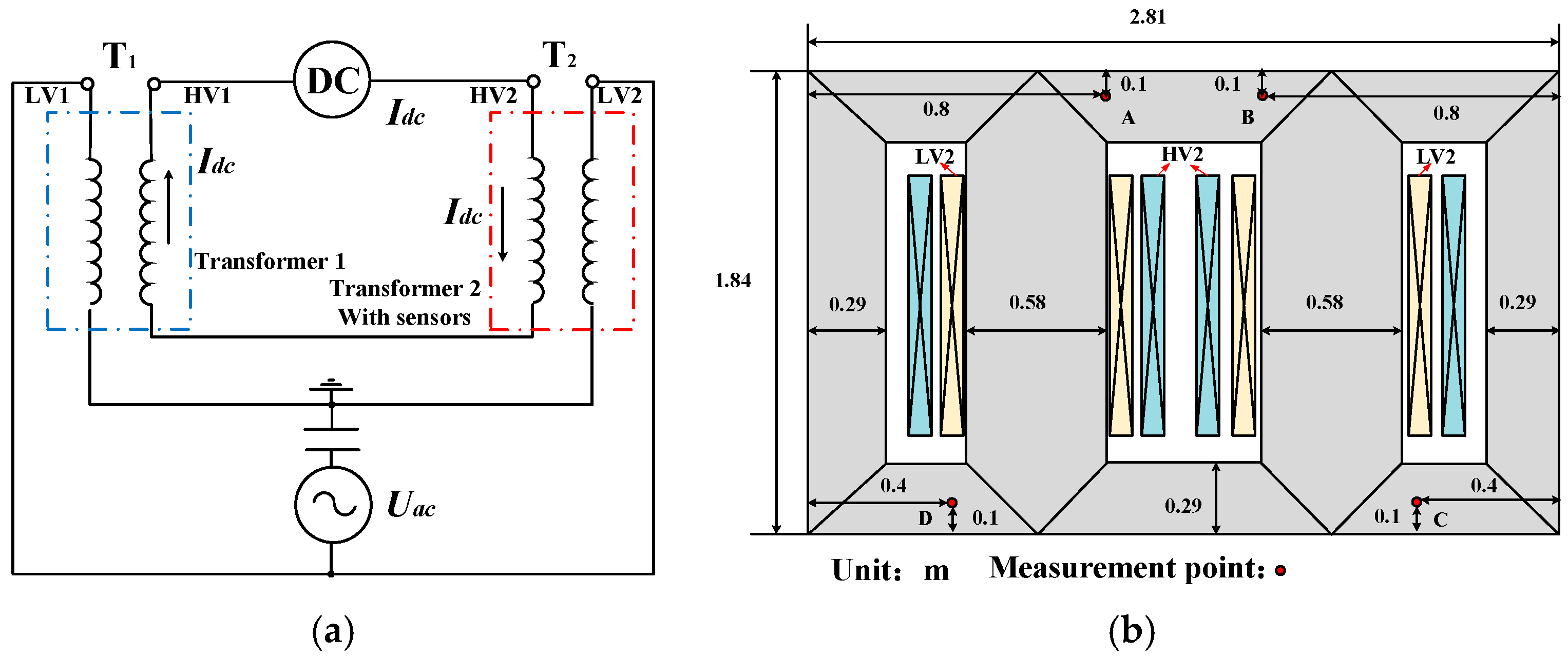
2.1. The Measurement Setup

The desired rotating magnetic field and the DC-biased field to be measured are shown in Figure 1a. The rotating magnetic field is defined by three parameters: the maximum value of the rotating magnetic field B_max, the incline direction angle θ, and the ratio α, which is the ratio of the minimum value B_min to the maximum value B_max, as follows: α = B_min/B_max. B_min is the minimum value at the B locus. The DC-biased field is characterized by two parameters: the amplitude B_dc and the direction θ_dc. The directions of the rotating magnetic field and DC-biased field are counted from the x-axis when θ and θ_dc are set as zero. The x-axis means the rolling direction and the y-axis means the traverse direction. In this study, a feedback measurement system for the rotating and DC-biased fields’ excitations and tests was established, as shown in Figure 1b. The system is composed of the single sheet tester (SST), the preamplifier (Krohn-Hite Model 7008, Brockton, MA, USA), the power amplifier (NF BP4610, Yokohama, Japan), and the multifunction I/O (Input/Output) device (USB-6353, Austin, TX, USA). The physical SST and the measurement system are shown in Figure 1c,d, respectively. The SST consists of two spatially orthogonal yokes, a pending test sample, and a B-H sensor. AC- and DC-biased excitations are sent from the I/O device, amplified by a power amplifier, and applied to the SST. The B and H signals detected by the B-H sensor are filtered and amplified by the preamplifier, and then sent back to the I/O device. The AC voltage for rotating magnetic field excitation and the DC voltage for DC-biased field excitation are simultaneously applied to the SST. The valid B and H signals, which consist of AC and DC components, respectively, are sensed based on Faraday’s law of induction and the boundary continuity effect of H. The DC components are extracted from the original B and H signals via an effective integration and filter process. The pending tested sample is a grain-oriented silicon steel with a square shape of 80 × 80 mm.

2.2. The Measured Magnetic Properties of 30ZH120

The grain-oriented electrical steel sheet 30ZH120 is commonly utilized in power transformer cores and serves as a test sample in this section. With the influence of different maximum magnetic flux values B_max and without DC-biased excitation, the loci of B and H are shown in Figure 2a,b, respectively. Here, B_x and H_x are the B and H components in the rolling direction, respectively, and B_y and H_y are the B and H components in the traverse direction. The B locus was controlled as an elliptical trajectory, and as B_max increased, the amplitudes of B_x, B_y, H_x and H_y also increased. Because of the nonlinear magnetization characteristics of the electrical steel sheet, the H locus distorts and is not an elliptical shape. The magnetization curve and permeability of 30ZH120 at the frequency 50 Hz in the easy magnetization direction are shown in Figure 2c. As H increases, B first rises rapidly and then tends to stabilize. Similarly, the corresponding permeability first increases and then decreases.

The waveforms and harmonic component amplitudes of B and H under the impact of different DC magnetic flux density amplitudes, B_dc, are shown in Figure 3. As B_dc increases, offset and asymmetric distortion occurs in the B_x, B_y, H_x and H_y waveforms. Under DC-biased field conditions, the amplitudes of the second harmonic components of B_x increase, whereas the amplitudes of the fundamental, second and third components of H_x increase. The harmonic component of B_x higher than 2nd is less than 0.03 T and is almost noise. The harmonic component of H_x higher than 4th is less than 1 A/m and is almost noise. The harmonic component amplitudes of B_y and H_y have the same trends as those of B_x and H_x. Increasing the harmonic component amplitudes of B and H waveforms could lead to a more significant eddy current effect and iron loss.

2.3. The Measured Iron Loss

Considering vectors B and vector H, iron core loss can be expressed as follows:

$$P_{iron}={\displaystyle \frac{1}{T_m\rho }}{\displaystyle \underset{0}{\overset{\mathrm{T}}{\int }}\mathit{H}\cdot \frac{d\mathit{B}}{dt}dt}={\displaystyle \frac{1}{T_m\rho }}{\displaystyle \underset{0}{\overset{\mathrm{T}}{\int }}(H_x\cdot \frac{d{B}_x}{dt}+H_y\cdot \frac{d{B}_y}{dt})dt}$$

(1)

where P_iron represents the iron core loss, T_m represents the magnetization period and ρ represents the electrical steel sheet density. The relationship between the loss of grain-oriented silicon steel and magnetization conditions (B_max, θ, α), as calculated using Equation (1) with a rotating magnetic field and without a DC-biased field, is shown in Figure 4a,b. This indicates that as B_max increases, the loss of the electrical steel sheet P_iron increases. When θ = 0°, the overall loss of the electrical steel sheet is relatively small, mainly because 0° is the rolling direction, which is the easy magnetization direction. As α increases, the rotational hysteresis loss of the electrical steel sheets increases, and the corresponding total loss increases. The relationship between the iron loss and the DC bias magnetization conditions (B_dc, θ_dc) is shown in Figure 4c. With the rise of B_dc, except for that of the rolling direction (θ_dc = 0°), the loss in other directions (θ_dc = 30°, 60° and 90°) first increases and then decreases. Moreover, since the directions (θ_dc = 60° and 90°) are difficult to magnetize, the rising and decreasing trend is more pronounced.

The loss in electrical steel sheets under different magnetization conditions can be further explained from the perspective of the magnetization process, magnetic domain movement and rotation, as shown in Figure 5 [24,25]. The magnetic domain behavior is described in Figure 5a under rotating field conditions for increasing values of B_max, ranging from 0.2 to 1.0 T, and changing values of θ and α. This description corresponds to the B-P_iron shown in Figure 4a,b. Owing to the applied rotating magnetic field direction changing, there are two simultaneous magnetization processes: magnetic domain movement and rotation. The amount of domain movement and rotation depends on the magnitude of the applied magnetic field H. Owing to the pinning of the domain by the defect sites inside the specimen, which causes an opposing force to resist any changes in B, there exists an angle difference between H and B. With a small rotating magnetic field, there is no disappearance or generation of the domain wall during the movement of the magnetic domain, and the rotational hysteresis loss is small and gradually increases with an increase in B_max. As the applied rotating field increases further, the magnetic domain, which was opposite to the direction of the magnetic field, disappears. As the magnetic field rotates, when the magnetic domain is not opposite the direction of the external magnetic field, it reappears, as shown in Figure 5a. Because the disappearance and generation of magnetic domain walls requires energy, the rotational hysteresis loss is rapid, and the corresponding total loss increases with an increase in B_max. Because the 60° and 90° directions are difficult to magnetize, many domain walls disappear and regenerate when the external magnetic field direction is rotated from 60° to 90°, leading to more iron loss, as shown in Figure 4a. When α = 0, the electrical steel sheet is under an alternating magnetic field, and the direction of the external magnetic field does not change, resulting in no rotational hysteresis loss and a relatively small total loss. As α increases, the magnetic field direction changes, and more magnetic domain walls in the difficult magnetization direction disappear and are generated again, resulting in an increasing rotational hysteresis loss and corresponding total loss, as shown in Figure 4b. The magnetic domain behavior is described in Figure 5b under rotating and DC-biased fields for increasing B_dc values, ranging from 0.2 to 1.0 T, and increasing θ_dc values from 0 to 90°, which corresponds to the B-P_iron relationship of Figure 4c. Under a rotating magnetic field and DC-biased magnetic field, as the amplitude of the external magnetic field further increases (corresponding to an increasing B_dc), more magnetic domain walls disappear and regenerate, leading to an increase in the loss of the electrical steel sheets. When the steel sheet is in a deep saturation state, the wall moves to the boundary interface of the magnetic domain, and the magnetic moment begins to rotate with the applied magnetic field to reduce the lag angle, as shown in Figure 5b. Owing to the fewer magnetic domains at this time, as the amplitude of B_dc increases, the corresponding total loss of the electrical steel sheets decreases. When θ_dc = 0°, the electrical steel sheet is not in the deep saturation state. Hence, the loss increases with the increasing B_dc.

3. Enhanced Dynamic Vector Hysteresis Model and Corresponding FEM Calculation

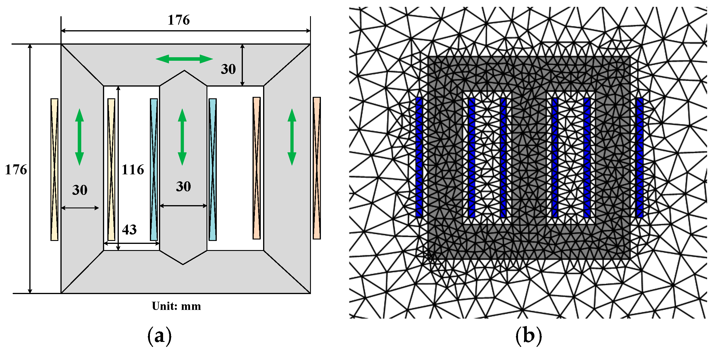
3.1. Governing Equation Derivation of the Two-Dimensional Magnetic Field and Temperature Field

The original vector magnetic hysteresis model was proposed to describe the behaviors of B and H only under a rotating field [19,20]. The nonlinear relationship between B and H can be expressed using an improved dynamic vector hysteresis model, as shown in Equation (2). The total magnetic field strength can be separated into three parts: the reduced magnetic field strength H_rek, the one caused by the eddy current H_exk and the one caused by the DC-biased field H_dck.

$$H_k(\tau )=H_{rek}(\tau )+H_{exk}(\tau )+H_{dck}=v_{rk}{B}_{ack}(\tau )+v_{hk}{\displaystyle \int B_{ack}(\tau )d}\tau +{\displaystyle \frac{\sigma \omega d^2}{12}}{\displaystyle \frac{d{B}_k}{d\tau }}+v_{0k}{B}_{dck}$$

(2)

where the time variable τ is a dimensionless time normalized by the period which can be expressed from the frequency and range from 0 to 2π; ω is the angular frequency of 50 Hz; σ is the resistivity; B_ack is the AC component of the B waveform; B_dck is the DC component of the B waveform; d is the thickness of the sheet, where the subscript k indicates x or y, which means that the parameters with the subscript k represent the corresponding components on the x- or y-axis. v_rk is the rotating reluctivity coefficient, v_hk is the rotating hysteresis coefficient and v_0k is the DC reluctivity coefficient. The H_rek and H_exk terms can be expressed using the following equations [21,22]:

$$H_{rek}(\tau )=v_{rk}{B}_{ack}(\tau )+v_{hk}{\displaystyle \int B_{ack}(\tau )d}\tau$$

(3)

$$H_{exk}(\tau )={\displaystyle \frac{\sigma \omega d^2}{12}}{\displaystyle \frac{d{B}_k}{d\tau }}$$

(4)

By combining the improved model with Maxwell’s equations, the governing equation of the two-dimensional magnetic field can be derived as follows:

$$\nabla \times {\mathit{v}}_{\mathit{r}}(\nabla \times {\mathit{A}}_{\mathit{a}\mathit{c}})+\nabla \times {\mathit{v}}_{\mathit{h}}{\displaystyle \int (\nabla \times {\mathit{A}}_{\mathit{a}\mathit{c}})d\tau }+\nabla \times {\displaystyle \frac{\sigma \omega d^2}{12}}{\displaystyle \frac{\partial (\nabla \times {\mathit{A}}_{\mathit{a}\mathit{c}})}{\partial \tau }}+\nabla \times {\mathit{v}}_{\mathbf{0}}(\nabla \times {\mathit{A}}_{\mathit{d}\mathit{c}})=\mathit{J}$$

(5)

where A_ac is the AC component of the magnetic vector potential, A_dc is the DC component of the magnetic vector potential and J is the excitation current density. Finite element discretization can be performed on the solution domain Ω_e, and Equation (5) can thus be re-written as follows:

$$\begin{array}{l}{\displaystyle \sum _E\left[{\displaystyle {\iint }_{{\Omega }_e}\left(\frac{\partial A_{ac}^e}{\partial y}\cdot v_{rx}\frac{\partial W^e}{\partial y}+\frac{\partial A_{ac}^e}{\partial x}\cdot v_{ry}\frac{\partial W^e}{\partial x}\right)dxdy}\right]}\\ \hspace{1em}\hspace{1em}+{\displaystyle \sum _E\left\{{\displaystyle \int \left[{\displaystyle {\iint }_{\Omega }\left(\frac{\partial A_{ac}^e}{\partial y}\cdot v_{hx}\frac{\partial W^e}{\partial y}+\frac{\partial A_{ac}^e}{\partial x}\cdot v_{hy}\frac{\partial W^e}{\partial x}\right)dxdy}\right]d\tau }\right\}}\\ \hspace{1em}\hspace{1em}\hspace{1em}+{\displaystyle \sum _E\left\{\frac{\sigma \omega d^2}{12}\frac{\partial }{\partial \tau }\left[{\displaystyle {\iint }_{\Omega }\left(\frac{\partial A_{ac}^e}{\partial y}\frac{\partial W^e}{\partial y}+\frac{\partial A_{ac}^e}{\partial x}\frac{\partial W^e}{\partial x}\right)dxdy}\right]\right\}}\\ \hspace{1em}\hspace{1em}\hspace{1em}\hspace{1em}+{\displaystyle \sum _E\left[{\displaystyle {\iint }_{{\Omega }_e}\left(\frac{\partial A_{dc}^e}{\partial y}\cdot v_{0x}\frac{\partial W^e}{\partial y}+\frac{\partial A_{dc}^e}{\partial x}\cdot v_{0y}\frac{\partial W^e}{\partial x}\right)dxdy}\right]}={\displaystyle \sum _E\left({\displaystyle {\iint }_{\Omega }{W}^e{J}^{e}dxdy}\right)}\end{array}$$

(6)

where W^e is the discretized weight function, the superscript e represents a single element and E is the total number of elements. The magnetic field distribution can be calculated by solving Equation (6). For a three-leg three-phase transformer core, by integrating the dynamic vector hysteresis model with finite element analysis, the distribution of magnetic parameters within the transformer core under a DC-biased field can be calculated. In this study, a DC-biased current was applied to the transformer winding, which implied that a DC-biased magnetic field was applied to the transformer core. The parameters (B_max, α, θ, B_dc and θ_dc) of rotating and DC-biased fields in each element are updated during each iteration of the FEM calculation. The corresponding v_r, v_h and v₀ in Equation (6) also change according to different parameters (B_max, α, θ, B_dc and θ_dc) during each iteration. Furthermore, a magnetization curve was introduced into the finite element analysis for comparison. The magnetic field distribution and the corresponding iron loss distribution are calculated in both cases: in which the magnetization curve is used and that in which an improved model is used.

The temperature rise caused by the winding loss can be conducted to the transformer core and exacerbates the local overheating problem under a DC bias. Therefore, in addition to the iron core, the copper loss from the winding generated under the DC-biased excitation should also be considered. The relationship between the copper loss and the current density J can be expressed as follows:

$$P_{coil}={\displaystyle \frac{J^2}{{\rho }_{coil}{\sigma }_{coil}}}$$

(7)

where P_coil and ρ_coil are the copper loss and density of the winding, respectively, and σ_coil represents the conductivity of copper. P_coil is included in both cases: in the case when the magnetization curve is used and in the case when an improved model is used.

Owing to the solid domain of the iron core and winding, the heat dissipation method involves heat conduction. The thermal convection effect of air in the calculation domain is ignored. According to Fourier’s law and the energy conservation law, under DC bias magnetization, the local loss and temperature change in the transformer iron core model satisfy the heat conduction governing equation, as follows:

$${\displaystyle \frac{\partial T}{\partial t}}={\displaystyle \frac{\lambda }{\rho C}}\left({\displaystyle \frac{{\partial }^{2}T}{\partial x^2}}+{\displaystyle \frac{{\partial }^{2}T}{\partial y^2}}\right)+{\displaystyle \frac{P}{C}}$$

(8)

where P represents the loss of iron core or winding, C indicates the specific heat capacity, λ is the heat transfer coefficient and T represents the temperature.

The space discretization is performed in the solution domain Ω_e, where Equation (8) could be expressed as follows:

$$\begin{array}{l}{\displaystyle \sum _E\left\{{\displaystyle {\iint }_{{\Omega }_e}\left[\frac{\partial W^e}{\partial x}\left(\frac{\lambda }{\rho }\frac{\partial T^e}{\partial x}\right)+\frac{\partial W^e}{\partial y}\left(\frac{\lambda }{\rho }\frac{\partial T^e}{\partial y}\right)\right]dxdy}\right\}}\\ \hspace{1em}\hspace{1em}\hspace{1em}\hspace{1em}\hspace{1em}\hspace{1em}\hspace{1em}\hspace{1em}\hspace{1em}\hspace{1em}\hspace{1em} +{\displaystyle \sum _E\left[{\displaystyle {\iint }_{{\Omega }_e}{W}^e\left(C\frac{\partial T^e}{\partial t}\right)dxdy}\right]}={\displaystyle \sum _E\left({\displaystyle {\iint }_{{\Omega }_e}{W}^e{P}^{e}dxdy}\right)}\end{array}$$

(9)

where T_e is the temperature of each element and P_e is the loss of each element.

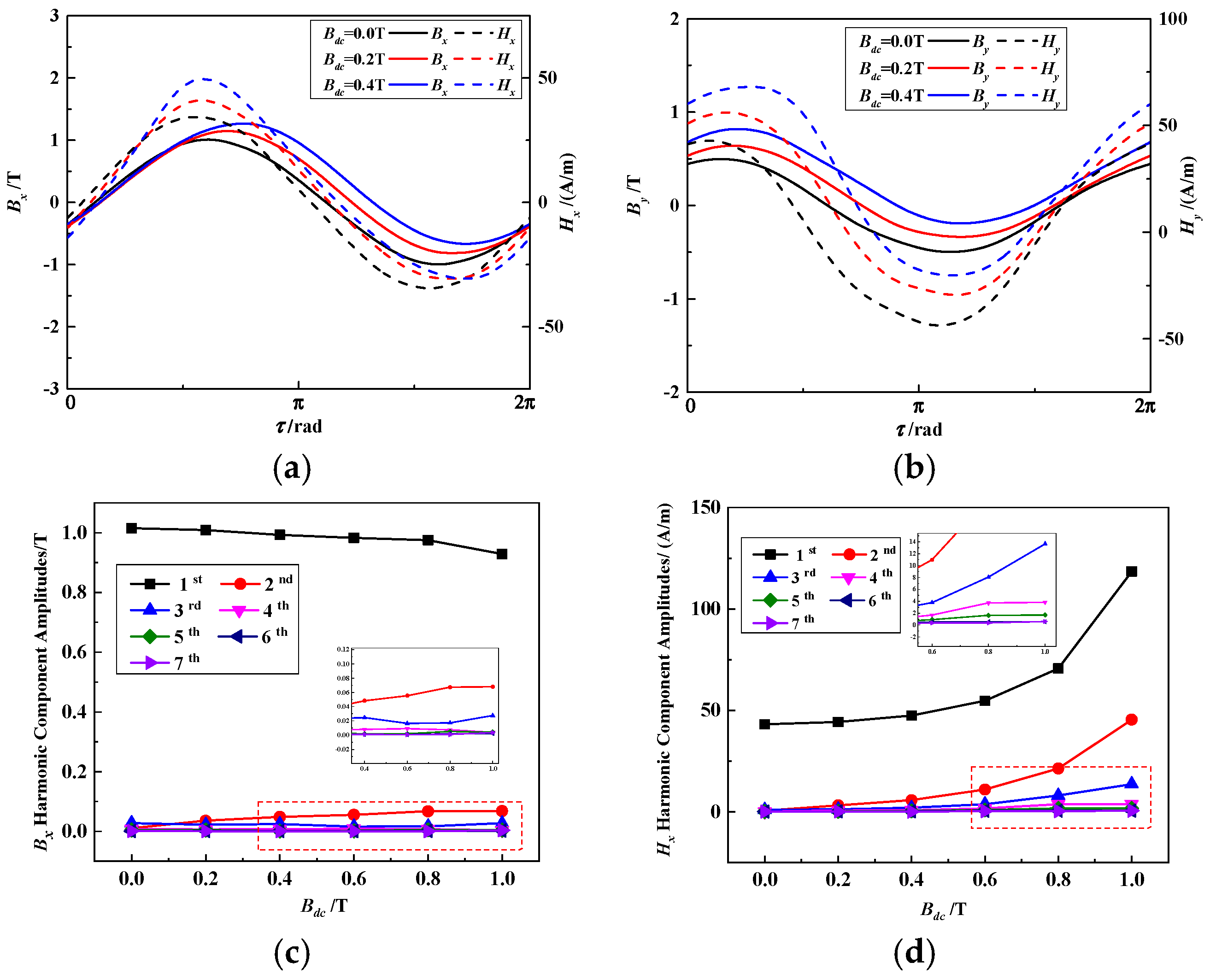
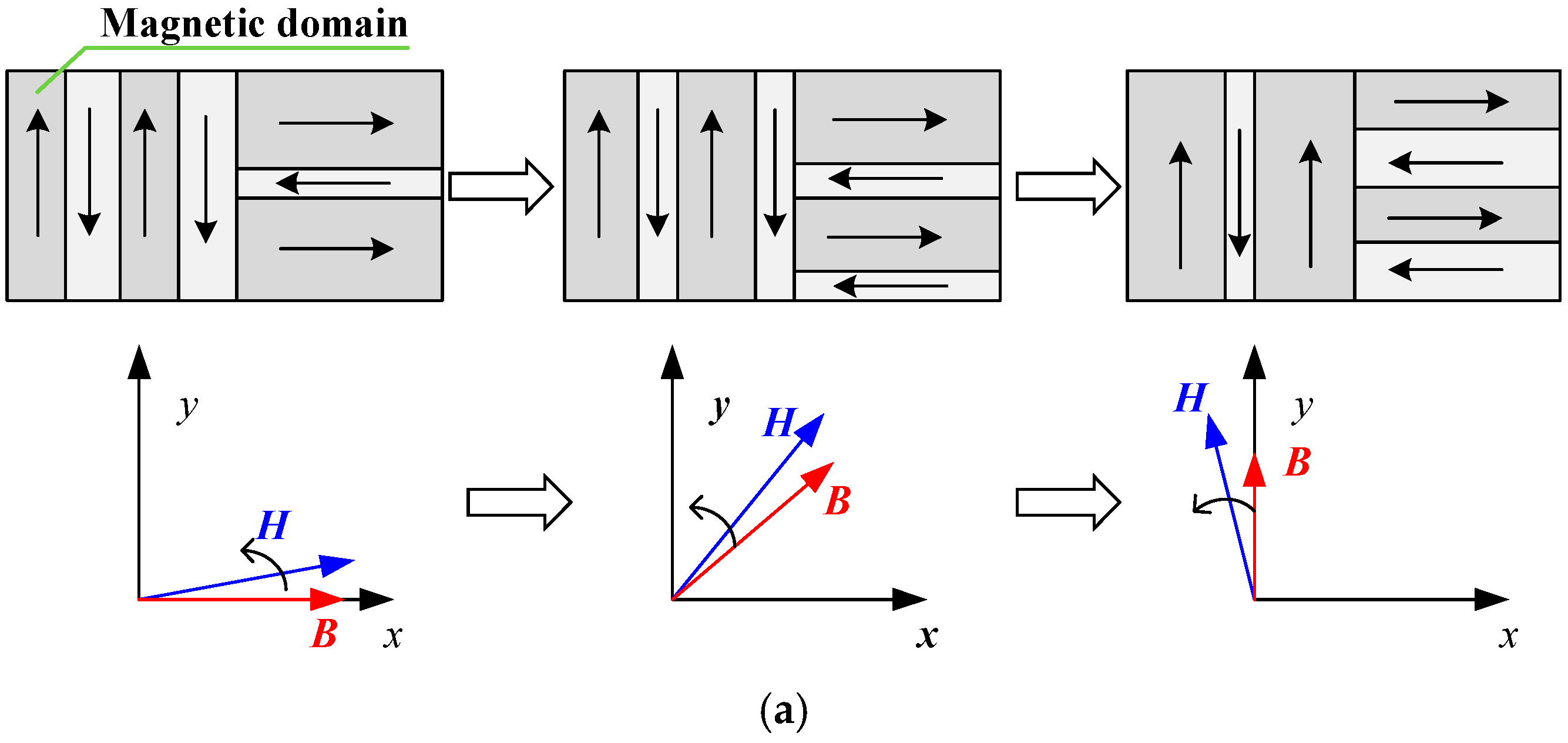
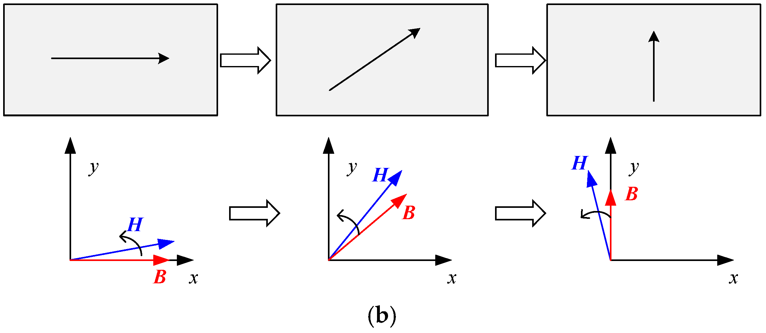
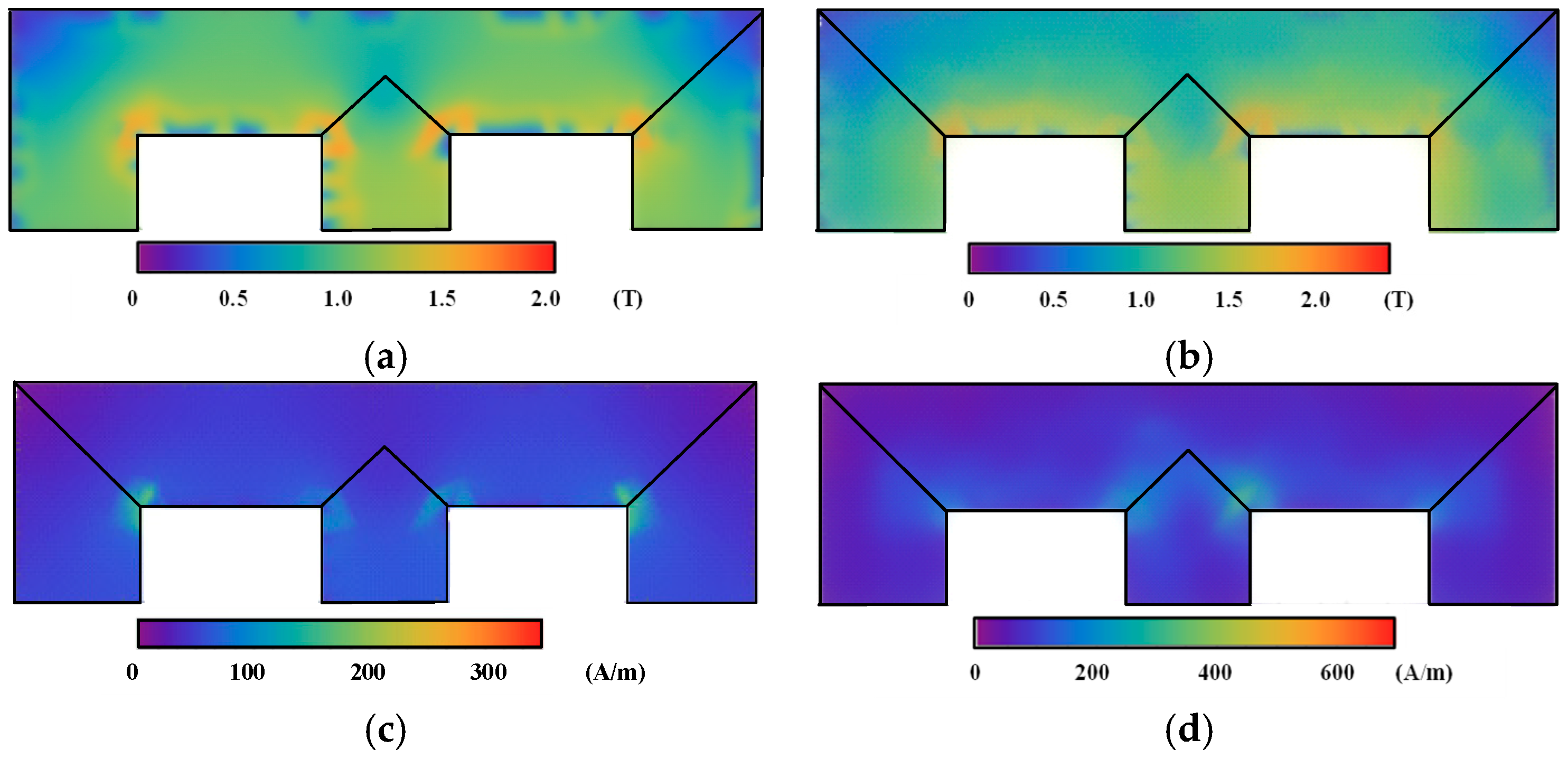
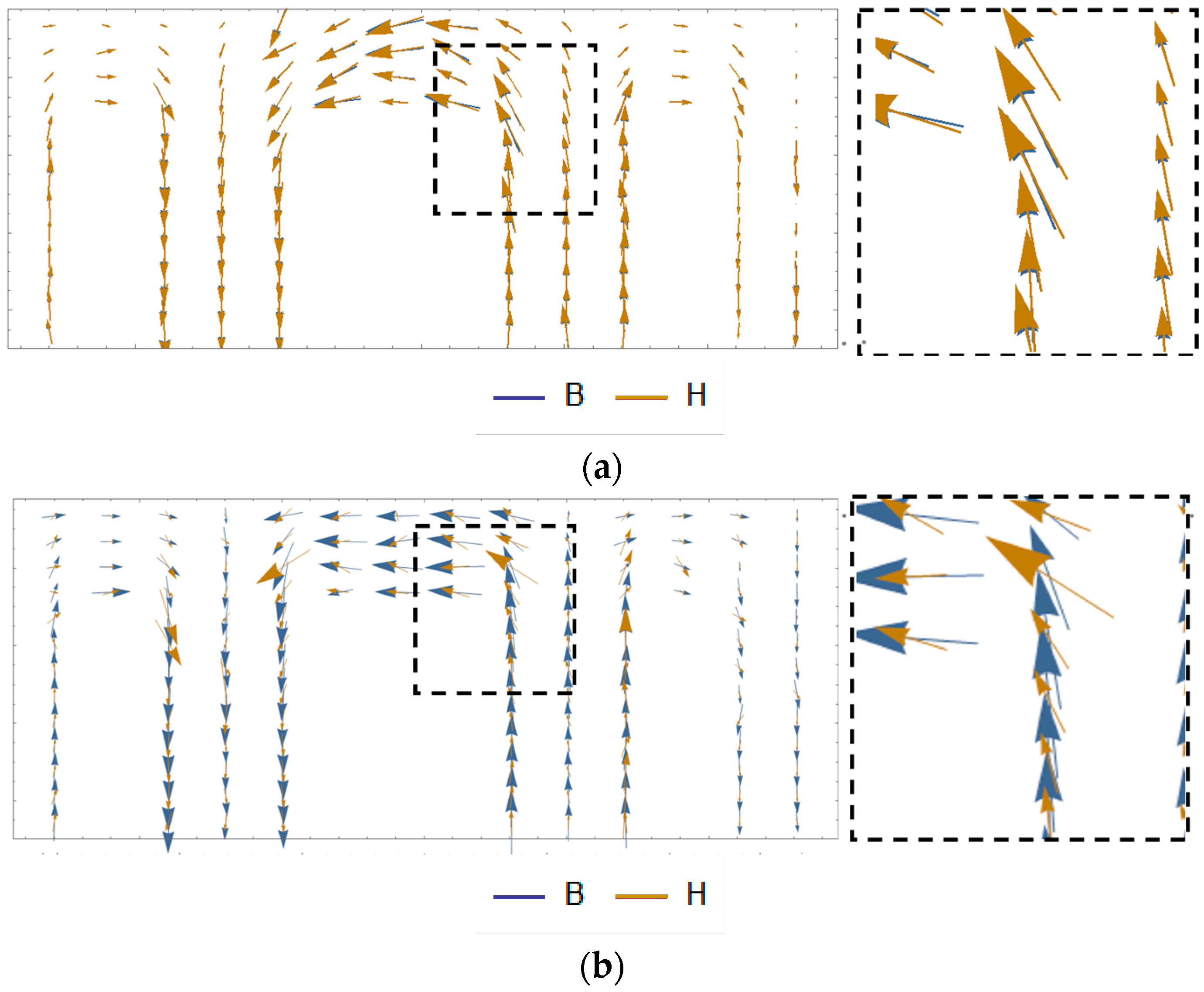
3.2. Analysis of the Magnetic Properties Distribution

A three-phase transformer core model was established for the FEM calculations under rotating and DC-biased fields. The transformer core model was made of multiple laminated, oriented 30ZH120 electrical steel sheets, ensuring that the direction of the iron yokes was parallel to the rolling directions of the electrical steel sheet, as shown in Figure 6a. The arrows indicate the rolling direction of electrical steel sheets. An AC excitation voltage with an amplitude of 3 V and a phase angle difference of 120° is applied to the three-phase winding, and a DC excitation voltage with an amplitude of 0.2 V is simultaneously applied to the left and right windings. The 2D automatic mesh with triangular elements on the three-phase transformer core model is shown in Figure 6b. The nonlinear governing Equations (6) and (9) were solved using the LinearSolve method. The FEM calculations were performed under Dirichlet boundary conditions.

Figure 7 illustrates the maximum values of B and H under DC-biased and rotating fields, respectively. The maximum value of B occurred at the upper window edge of the iron core, which was caused by the concentration of the magnetic force line. Compared with those of magnetization curve, the maximum value of H in the improved model was 251 A/m and was larger than that of the magnetization curve (173 A/m). This is because the hysteresis and eddy current effects of the rotating magnetic field are neglected in the FEM calculation of the magnetization curve.

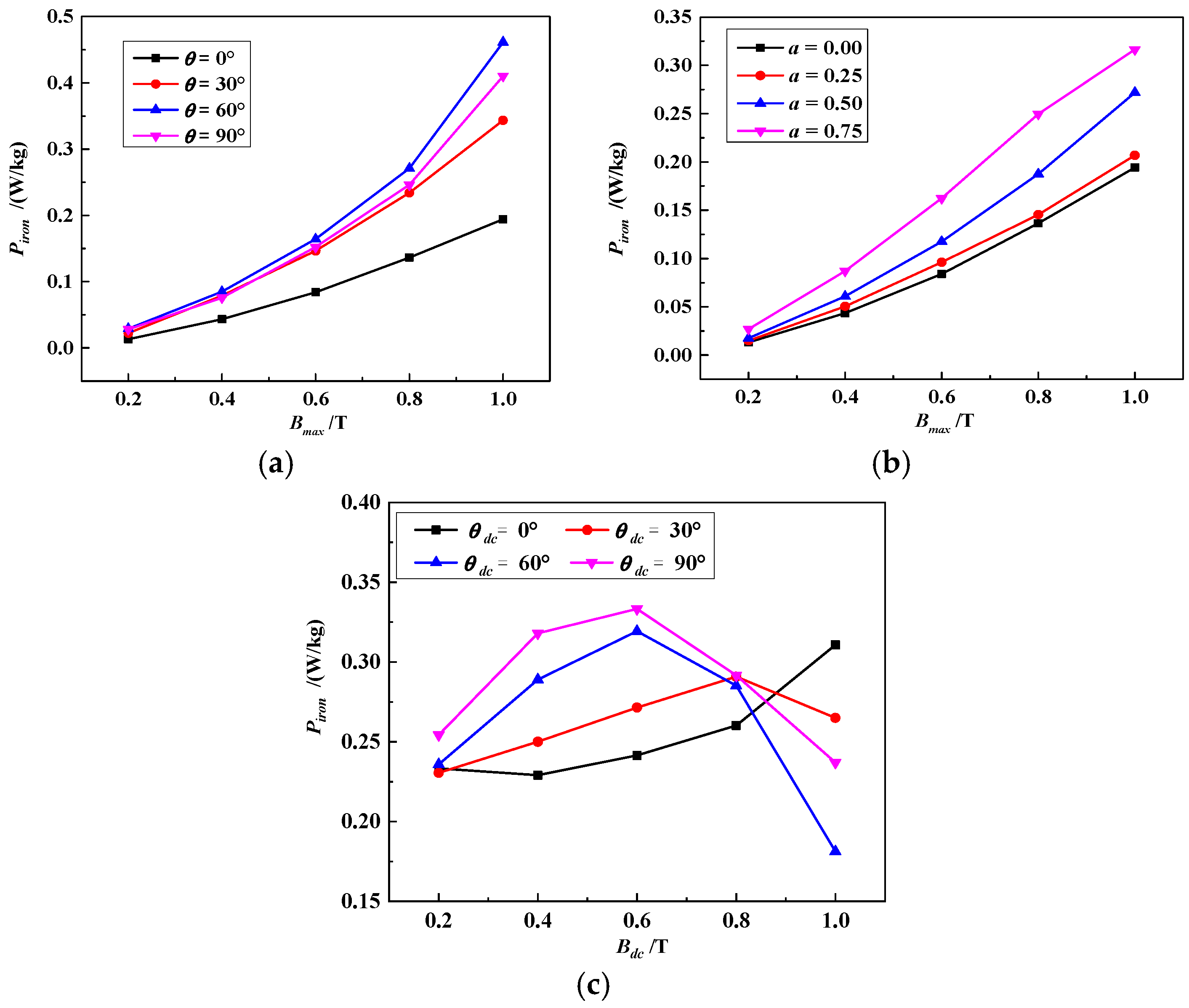
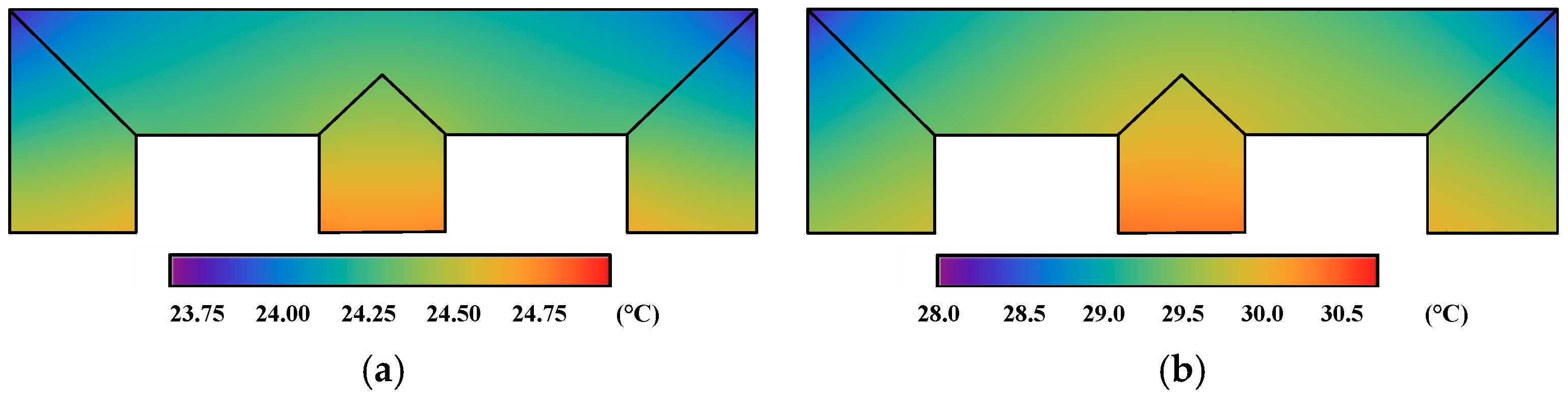
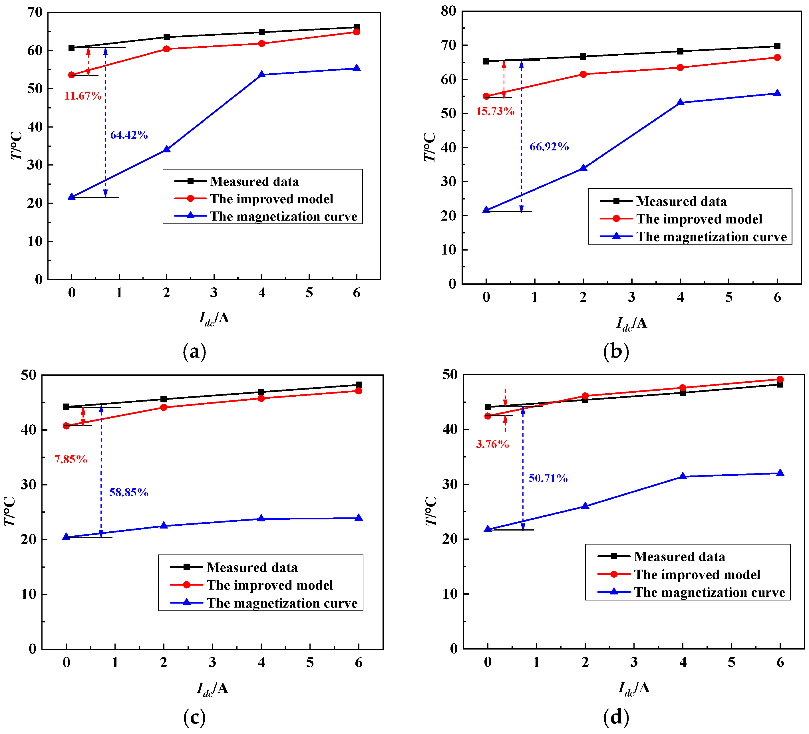
3.3. Analysis of Core Loss and the Temperature

Figure 8 shows the distribution of the iron core loss under DC bias magnetization, as calculated using the magnetization curve and dynamic vector hysteresis model. The maximum loss calculated by the magnetization curve is 0.321 W/kg·m, and that calculated by the dynamic model is 1.652 W/kg·m. Owing to the influence of the rotating magnetic field and the hysteresis effect of the electrical steel sheet, compared with the magnetization curve, the core loss under DC bias, as calculated by the dynamic vector hysteresis model, has larger values at the corners and T-joint area of the transformer core model.

The uneven distribution of the iron core losses in Figure 8 and the winding loss were applied as the heat source load, and the temperature distribution of the transformer iron core model under DC bias was calculated using the magnetization curve and dynamic vector hysteresis model, as shown in Figure 9. The original temperature is the room temperature, 20 °C. Owing to the impacts of the copper loss of the winding and the heat conduction effect, the hottest point of the iron core model was near the middle core limb position.

The corner temperature calculated by the magnetization curve increases by 4.29 °C, and the T-joint area increases by 4.41 °C. At the same position, the corner temperature calculated by the dynamic model increases by 9.60 °C, and the T-joint area increases by 9.91 °C. The overall temperature calculated by the dynamic model is about 5 °C higher than that calculated by the magnetization curve. This is mainly because the dynamic model considers the influence of the rotating magnetic field and hysteresis effect, resulting in a higher calculated iron core loss. Additionally, compared with those in the rolling direction, the values of H, iron loss and temperature calculated by the magnetization curve in traverse direction would be larger, since the steel sheet is harder to magnetize in this direction. The magnetization curve in a different direction would be applied in the FEM calculation and would be further analyzed in follow-up research.

4. Verification of the FEM Calculation

To verify the reliability of the FEM calculation, the temperature distribution test results for a 110 kV single-phase autotransformer power transformer under a DC bias are utilized as comparative data. The measured excitation current is applied as the input for the numerical analysis, and the distribution of the magnetic parameters in the power transformer core under a DC bias is calculated. Furthermore, the iron loss and temperature increase are calculated and compared with the measurement results of the DC bias test of the physical power transformer. The single-phase transformer is highly sensitive to DC magnetic flux. Therefore, 110 kV single-phase autotransformer power transformer is selected as the tested subject. The main technical parameters of the tested transformer are listed in

Table 1. The main technical parameters of the tested transformer.

Technical Parameters		Value	Technical Parameters		Value
Electrical parameters	Rated voltage	$110/\sqrt{3}\pm 10\%/10.5\mathrm{kV}$	Low-voltage side winding	Winding method	Continuous
	Rated capacity	21 MVA		Number of turns	112
High-voltage side winding	Winding method	Sandwich-interleaved	Iron core	Brand	27RK090
	Number of turns	583~729		Structure	Single-phase four-limb

.

The connection mode of the DC magnetic bias test for power transformers is illustrated in Figure 10a. Two 110 kV power transformers are connected in parallel on the high-voltage side, and the low-voltage side is also connected in parallel. The transformer is equipped with sensors to measure the local temperature increase. Transformer 1 does not contain sensors and is tapped negatively, whereas Transformer 2 is tapped positively. Owing to the different turns of the high-voltage winding, there is a circulating current on the low-voltage side, which means that Transformer 2 is in operation state. The DC bias excitation is introduced from the high-voltage side winding of the transformer, so that Transformer 2 operates in a DC-biased state.

The transformer structure is shown in Figure 10b. The windings on the high-voltage (HV2) and low-voltage (LV2) sides are mounted around the two main limbs. T-type thermocouples are embedded in the T-joint area on the surfaces of the two main limbs of the transformer core to measure the local temperature increase under DC bias magnetization, since this area is more sensitive to the rotating magnetic field. The original temperature is the room temperature, 20 °C. The currents of the high- and low-voltage windings of the transformer are measured, and the corresponding excitation current is obtained, as shown in Figure 11a. The exciting current in Figure 11a is directly introduced into the transformer core in the FEM calculation to simulate the DC-biased situation of different I_dc values (I_dc = 0, 2, 4 and 6 A). The core of the 110 kV single-phase autotransformer power transformer is made of a grain-oriented 27RK090 electrical steel sheet. The magnetization curve and corresponding permeability of 27RK090 of the frequency 50 Hz in the easy magnetization direction are shown in Figure 11b. The experimental data are presented in [26].

The 2D automatic mesh with triangular elements is applied to the physical transformer core, as shown in Figure 12. The magnetic property distribution and corresponding loss and temperature rise distributions can be obtained by solving the nonlinear governing Equations (6) and (9) via the LinearSolve method.

The distributions of B and H calculated using the dynamic model and the basic magnetization curve are shown in Figure 13, where I_dc = 6 A. For the magnetization curve, B is parallel to H, but there is an angle lag between the calculated B and H of the dynamic model at the T-shaped connection and corner of the transformer core, which is the characteristic of the rotating magnetic field that is considered in the proposed model.

The temperature distribution of the transformer iron core with I_dc = 6 A is calculated using the magnetization curve and dynamic vector hysteresis model, as shown in Figure 14. These results indicate that the maximum temperature occurred in the main limb area of the transformer core, which is related to the heat conduction of the winding. Compared with the magnetization curve, the temperature of the proposed model considering the hysteresis and eddy current effects has a larger value.

To verify the local temperature rise of the transformer core at points A, B and C under different I_dc values (I_dc = 0, 2, 4 and 6 A), the waveforms of the vector magnetic flux density and vector magnetic field intensity in a magnetization period and the corresponding core loss are calculated using the dynamic vector hysteresis model and basic magnetization curve under a DC bias, as shown in

Table 2. Local losses of transformer core at Points A, B, C and D.

Core Loss P/(W/kg)	Point A		Point B		Point C		Point D
	Dynamic Model	Magnetization Curve	Dynamic Model	Magnetization Curve	Dynamic Model	Magnetization Curve	Dynamic Model	Magnetization Curve
Idc = 0 A	2.092	0.099	2.179	0.100	1.290	0.025	1.182	0.020
Idc = 2 A	2.514	0.871	2.582	0.862	1.501	0.154	1.523	0.141
Idc = 4 A	2.602	2.092	2.704	2.062	1.602	0.234	1.716	0.251
Idc = 6 A	2.791	2.198	2.888	2.233	1.687	0.242	1.762	0.269

.

As I_dc increases, the half-wave saturation in the transformer core becomes more pronounced, which causes the H waveform to peak, indicating a stronger hysteresis effect. Consequently, the corresponding local losses at points A, B, C and D, as calculated using the dynamic model and magnetization curve, also increase. Points A and B are situated in the main magnetic circuit of the transformer core, whereas points C and D are in the iron core bypass. The magnitudes of B and H in the main magnetic circuit are higher than those in the bypass circuit. Therefore, the calculated loss values of points A and B of the dynamic model and the magnetization curve are higher than the those of points C and D. Considering the hysteresis and eddy current effects of rotating magnetic field and DC-biased field in the dynamic model, the local loss value of the proposed model is larger than that of the magnetization curve.

To verify the finite element calculation results of the power transformer core considering the dynamic vector hysteresis model under a DC magnetic bias, it is necessary to compare the temperature changes at points A, B, C and D under different DC bias conditions with the measured data, as shown in Figure 15. During the DC bias test, different I_dc values are applied to the transformer for 2 h to measure stable and accurate temperature values using a T-type thermocouple. The calculated results are obtained by combining the finite element analysis with the magnetization curve and using the dynamic model and the magnetization curve. As I_dc increases, the transformer core experiences the half-wave saturation, thereby leading to an increase in core losses. Consequently, the calculated temperatures at points A, B, C and D of both the magnetization curve and the dynamic model increase. The temperatures at points A and B are higher than those at points C and D. This is because B and H in the main magnetic circuit are higher than those in the bypass circuit. Because the hysteresis effect and anisotropy of the transformer core under a rotating magnetic field and DC-biased field are considered in the improved model, the local temperature calculated by the dynamic model is higher than that calculated by the magnetization curve, and is more consistent with the measured data. The calculated errors of the temperature increase at points A, B, C and D are listed in

Table 3. The calculated error of temperature rise at Points A, B, C and D.

Calculated Error	Point A		Point B		Point C		Point D
	Dynamic Model	Magnetization Curve	Dynamic Model	Magnetization Curve	Dynamic Model	Magnetization Curve	Dynamic Model	Magnetization Curve
Idc = 0 A	11.67%	64.42%	15.73%	66.92%	7.85%	53.84%	3.76%	50.71%
Idc = 2 A	4.88%	46.45%	7.81%	49.23%	3.28%	50.72%	1.56%	42.81%
Idc = 4 A	4.60%	17.25%	6.95%	22.08%	2.45%	49.33%	1.92%	32.78%
Idc = 6 A	1.89%	16.29%	4.717%	19.81%	2.26%	50.45%	1.98%	33.58%

. The calculation error of the proposed model ranges from 3.76 to 15.73%, which is far less than the error of the magnetization curve (approximately 50.71–66.92%). These results demonstrate that the FEM calculation results of the dynamic vector hysteresis model, which considers the impact of hysteresis and eddy current effects under a DC bias, can provide more accurate temperature estimations than those of the basic magnetization curve.

To simplify the FEM analysis, only the influences of the iron core loss and winding copper loss are considered in this study, and the influence of the stray loss of the metal structural components is neglected in the temperature rise calculation. Therefore, the calculation error of the proposed model reaches a maximum value of 15.73%. The impact of the stray loss of the metal structural components on the temperature rise of the transformer core will be discussed in further research. In addition, because of the difficulty in measuring the local vector magnetic parameters and losses of the transformer cores, only the local temperature rise is calculated and verified using the experimental data in this study. An improved method for the local magnetic parameters detection of the transformer core will be studied, and the FEM results calculated by the proposed vector model will be further verified in future research.

Owing to the large volume and high voltage levels of actual ultrahigh-voltage transformers, the amplitude of the current flowing through the neutral point of the winding under a DC bias is large. Therefore, compared with the transformer tested in this study, the local overheating temperature of ultrahigh-voltage transformers under a DC bias is higher, and further DC bias isolation protection in the power network is indispensable.

5. Conclusions

In this study, an improved dynamic vector hysteresis model that considers the hysteresis and eddy current effects was introduced into the FEM analysis of the iron loss and temperature distribution of a transformer core under a DC-biased field. A measurement system for the magnetic characteristics under rotating and DC-biased fields was established, and the iron loss was measured under different DC-biased magnetization conditions. As the magnetic domain vanished, regenerated and moved, the iron loss first increased and then decreased with the increasing B_dc. An enhanced model was established by introducing reduced magnetic field strengths, one caused by eddy current and one caused by a DC-biased field. The proposed model was combined with a numerical analysis to simulate the distribution of magnetic properties, iron loss and temperature. The maximum values of the H and the iron loss occurred at the corners and T-joint of the core, and the temperature was higher in the main limb area. The FEM calculation results were verified using the temperature rise data of the 110 kV power transformer. Compared with the magnetization curve, the temperature distribution of the proposed model, with a calculation error ranging from 3.76 to 15.73%, was more accurate and reliable. The calculation error would be minimized with consideration of the stray loss of metal structural components in further research. The local temperature of a transformer core can exceed 65 °C when I_dc = 6 A, indicating that DC bias isolation protection is indispensable in the power network.

References

1. Etemadi, A.H.; Rezaei-Zare, A. Optimal placement of GIC blocking devices for geomagnetic disturbance mitigation. IEEE Trans. Power Syst. 2014, 29, 2753–2762. [Google Scholar] [CrossRef]
2. Fang, X.; Ma, D.; Zhao, T.; Fan, W.; Quan, W.; Xiao, Z.; Zhai, Y. Accurate and fast measurement of alkali-metal and noble-gas atoms spin polarizability based on frequency response in SERF co-magnetometer. Measurement 2023, 222, 113562. [Google Scholar] [CrossRef]
3. Fang, X.; Wei, K.; Zhai, Y.; Zhao, T.; Chen, X.; Zhou, M.; Liu, Y.; Ma, D.; Xiao, Z. Analysis of effects of magnetic field gradient on atomic spin polarization and relaxation in optically pumped atomic magnetometers. Opt. Express 2022, 30, 3926–3940. [Google Scholar] [CrossRef] [PubMed]
4. Larsen, E.V.; Nordell, D.E.; Ponder, J.; Albertson, V.D.; Bozoki, B.; Feero, W.E.; Kappenman, J.G.; Prabhakara, F.S.; Thompson, K.; Walling, R. Geomagnetic disturbance effects on power systems. IEEE Trans. Power Deliv. 1993, 8, 1206–1216. [Google Scholar]
5. Lu, J.; Wang, S.; Lu, F.; Lu, C.; Zhang, X.; Ma, D. Hybrid optimal design of square highly uniform magnetic field coils. IEEE Trans. Ind. Electron. 2023, 70, 4236–4244. [Google Scholar] [CrossRef]
6. Pulkkinen, A.; Lindahl, S.; Viljanen, A.; Pirjola, R. Geomagnetic storm of 29–31 October 2003: Geomagnetically induced currents and their relation to problems in the Swedish high—voltage power transmission system. Space Weather 2005, 3, 1–19. [Google Scholar] [CrossRef]
7. Li, Y.; Luo, Z. A comparative study of J–A and Preisach improved models for core loss calculation under DC bias. Sci. Rep. 2024, 14, 9409. [Google Scholar] [CrossRef]
8. Yao, Y.; Chang, S.K.; Ni, G.; Xie, D. 3-D nonlinear transient eddy current calculation of online power transformer under DC bias. IEEE Trans. Magn. 2005, 41, 1840–1843. [Google Scholar]
9. Shi, M.; Qiu, A.; Li, J. Vector magnetic properties of electrical steel sheet under DC-biased flux and rotating magnetic fields of varying frequencies. IEEE Trans. Magn. 2021, 57, 7503704. [Google Scholar] [CrossRef]
10. Wei, W.; Arne, N.; ·Niklas, M. Common and differential mode of DC-bias in three-phase power transformers. Electr. Eng. 2022, 104, 3993–4004. [Google Scholar]
11. Enokizono, M.; Soda, N. Finite element analysis of transformer model core with measured reluctivity tensor. IEEE Trans. Magn. 1997, 33, 4110–4112. [Google Scholar] [CrossRef]
12. Shi, M.; Zhang, X.; Yang, J.; Yuan, S.; Wang, L. An optimized measurement method for magnetic properties of permalloy sheet under demagnetization. IEEE Trans. Instrum. Meas. 2022, 71, 1–9. [Google Scholar] [CrossRef]
13. Enokizono, M. Vector magneto-hysteresis E&S model and magnetic characteristic analysis. IEEE Trans. Magn. 2006, 42, 915–918. [Google Scholar]
14. Bergqvist, A.J. A simple vector generalization of the Jiles-Atherton model of hysteresis. IEEE Trans. Magn. 1996, 32, 4213–4215. [Google Scholar] [CrossRef]
15. Chen, J.; Wang, S.; Shang, H.; Hu, H.; Peng, T. Finite element analysis of axial flux permanent magnetic hysteresis dampers based on vector Jiles-Atherton model. IEEE Trans. Energy Convers. 2022, 37, 2472–2481. [Google Scholar] [CrossRef]
16. Torre, E.D. Preisach modeling and reversible magnetization. IEEE Trans. Magn. 1990, 26, 3052–3058. [Google Scholar] [CrossRef]
17. Riccardo, S.; Riganti-Fulginei, F.; Laudani, A.; Quandam, S. Algorithms to reduce the computational cost of vector Preisach model in view of Finite Element analysis. J. Magn. Magn. Mater. 2022, 546, 168876. [Google Scholar] [CrossRef]
18. Soda, N.; Enokizono, M. E&S hysteresis model for two-dimensional magnetic properties. J. Magn. Magn. Mater. 2000, 215–216, 626–628. [Google Scholar]
19. Shimoji, H.; Enokizono, M.; Todaka, T.; Honda, T. A new modeling of the vector magnetic property. IEEE Trans. Magn. 2002, 38, 861–864. [Google Scholar] [CrossRef]
20. Urata, S.; Enokizono, M.; Todaka, T.; Shimoji, H. Magnetic characteristic analysis of the motor considering 2-D vector magnetic property. IEEE Trans. Magn. 2006, 42, 615–618. [Google Scholar] [CrossRef]
21. Kunihiro, N.; Todaka, T.; Enokizono, M. Loss evaluation of an induction motor model core by vector magnetic characteristic analysis. IEEE Trans. Magn. 2011, 47, 1098–1101. [Google Scholar] [CrossRef]
22. Yokoyama, D.; Sato, T.; Todaka, T.; Enokizono, M. Comparison of Iron Loss Characteristics of Divided Cores Considering Vector Magnetic Properties. IEEE Trans. Magn. 2014, 50, 1–4. [Google Scholar] [CrossRef]
23. Shi, M.; Yang, Y. An improved vector hysteresis model incorporating the effect of DC-biased field and its application to FEM analysis of three-limb transformer core. J. Electr. Eng. Technol. 2024, 1–12. [Google Scholar] [CrossRef]
24. Xu, W. Numerical Simulation and Experimental Verification on the Vectorial Magnetic Hysteresis of Electromagnetic Materials. Ph.D. Thesis, Xi’an Jiaotong University, Xi’an, China, 2017. [Google Scholar]
25. Zhu, J. Numerical Modelling of Magnetic Materials for Computer Aided Design of Electromagnetic Devices. Ph.D. Thesis, University of Technology, Sydney, Australia, 1994. [Google Scholar]
26. Zhang, S.; Wang, K.; Li, J.; Sun, J.; Xie, Q.; Hu, X. Tests of DC bias key performances of power transformer with single-phase three-limb core under no-load and rated-load conditions. Proc. CSEE 2019, 39, 4334–4344. [Google Scholar]
Figure 1. The desired field and the feedback measurement system: (a) Desired field. (b) Schematic of the experimental measurement system. (c) The physical single sheet tester (SST). (d) The physical measurement system.
Materials 17 03767 g001
Figure 2. Loci of B and H under different Bmax without DC bias and the corresponding magnetization curve and permeability of 30ZH120: (a) B locus. (b) H locus. (c) Magnetization curve and permeability of 30ZH120 at the frequency 50 Hz in easy magnetization direction.
Materials 17 03767 g002
Figure 3. Waveforms and harmonic component amplitudes of B and H under different Bdc: (a) Bx and Hx waveforms. (b) By and Hy waveforms. (c) Bx harmonic component amplitudes. (d) Hx harmonic component amplitudes.
Materials 17 03767 g003
Figure 4. The iron loss under different magnetization conditions: (a) The loss of different Bmax and θ. (b) The loss of different Bmax and α. (c) The loss of different Bdc.
Materials 17 03767 g004
Figure 5. The movement process of magnetic domain: (a) The movement process of magnetic domain under the rotating magnetic field increasing for Bmax ranging from 0.2 to 1.0 T. (b) The movement process of magnetic domain under the rotating magnetic field and DC-biased field for increasing Bdc ranging from 0.2 to 1.0 T and increasing θdc from 0 to 90°.
Materials 17 03767 g005aMaterials 17 03767 g005b
Figure 6. Transform core model and the mesh: (a) The transform core model. (b) The mesh.
Materials 17 03767 g006
Figure 7. Distribution of the maximum value of B and H of the transformer core model: (a) Maximum value of B calculated using the magnetization curve. (b) Maximum value of B calculated using the improved model. (c) Maximum value of H calculated using the magnetization curve. (d) Maximum value of H calculated using the improved model.
Materials 17 03767 g007
Figure 8. Distribution of iron loss of the transformer core model: (a) Iron loss calculated using the magnetization curve. (b) Iron loss calculated using the improved model.
Materials 17 03767 g008
Figure 9. Distribution of temperature of the transformer core model: (a) Temperature calculated using the magnetization curve. (b) Temperature calculated using the improved model.
Materials 17 03767 g009
Figure 10. Schematic diagram of DC bias test: (a) Wiring schematic diagram for DC bias test. (b) Temperature rise measurement point for DC bias magnetic test.
Materials 17 03767 g010
Figure 11. Exciting current and magnetization curve of the tested transformer core: (a) Exciting current for different DC bias conditions. (b) Magnetization curve and the corresponding permeability of 27RK090 (50 Hz) of the tested transformer core in easy magnetization direction.
Materials 17 03767 g011
Figure 12. The 2D automatic mesh with triangular elements of the physical transformer core.
Materials 17 03767 g012
Figure 13. Distribution of B and H of the physical 110 kV transformer core: (a) Distribution of B and H calculated using the basic magnetization curve. (b) Distribution of B and H calculated using proposed model.
Materials 17 03767 g013
Figure 14. Distribution of temperature of the physical 110 kV transformer core: (a) Temperature calculated using the magnetization curve. (b) Temperature calculated using the improved model.
Materials 17 03767 g014
Figure 15. Comparison between calculated and measured values of local temperature of iron core: (a) Point A. (b) Point B. (c) Point C. (d) Point D.
Materials 17 03767 g015