

Sliding Shear Failure of Basement-Clamped Reinforced Concrete Shear Walls


Abstract
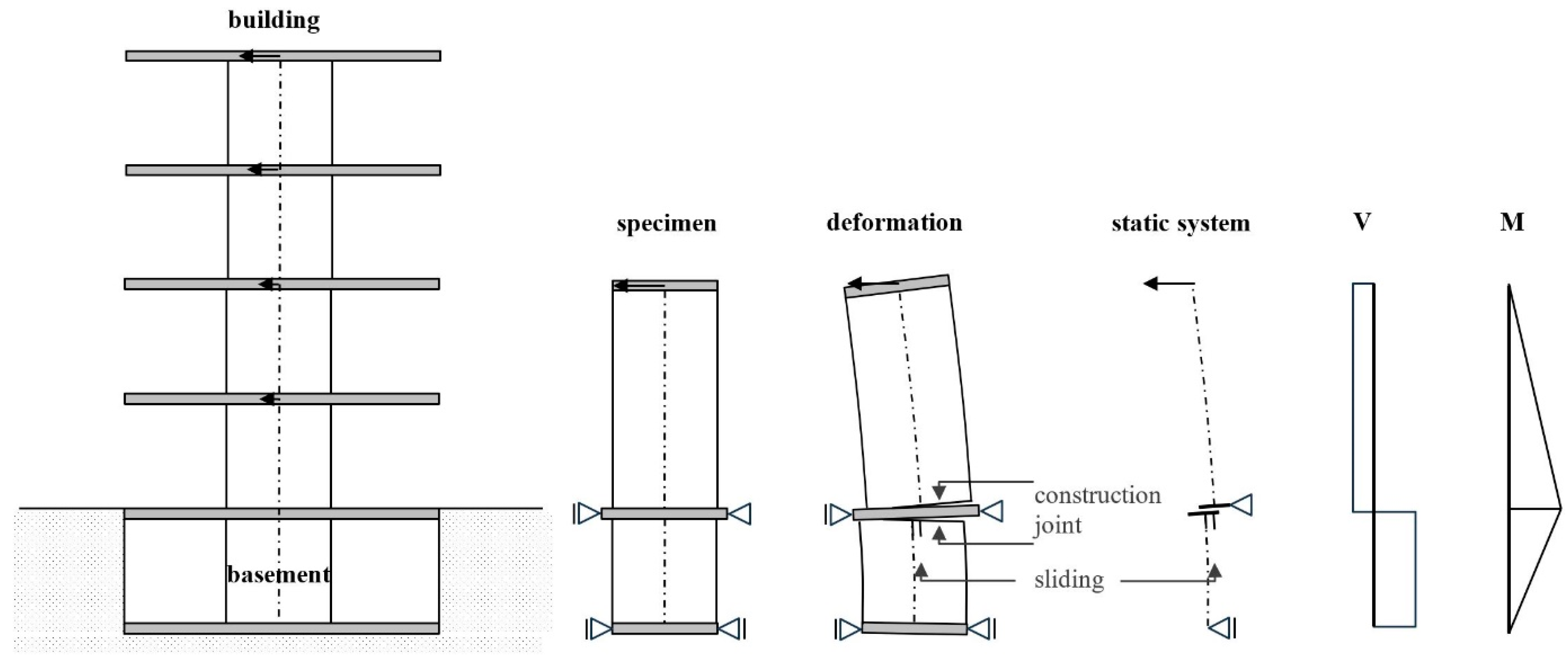
1. Introduction
- -
- Where are flexural cracks localised and how do they initiate sliding shear failure? How advanced is the deformation and the plastic strain around the construction joint before sliding shear displacements occur?
- -
- How is the friction resistance in the compression zone of the construction joint? How is the friction resistance in a zone in which the cracks do not close completely when the load is reversed?
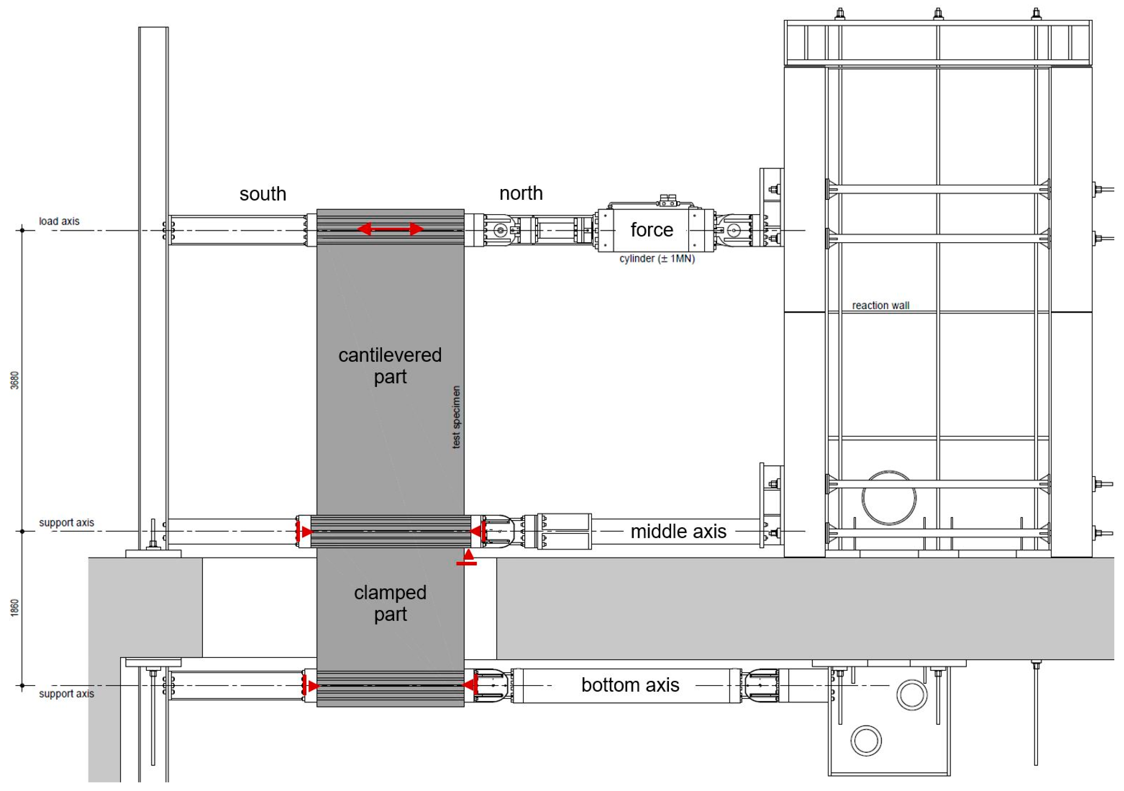
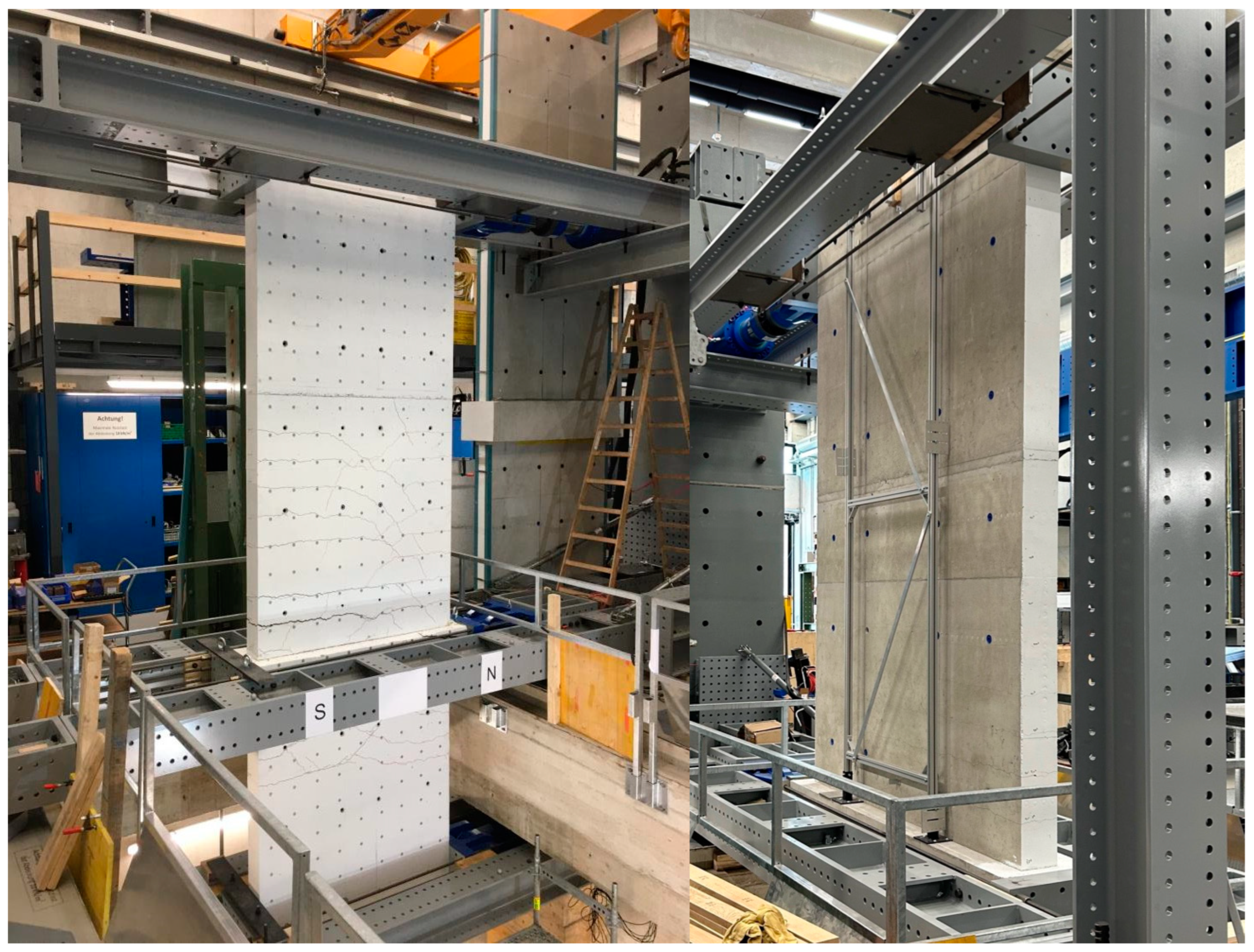
2. Experimental Set-Up and Test Specimens
2.1. Experimental Set-Up
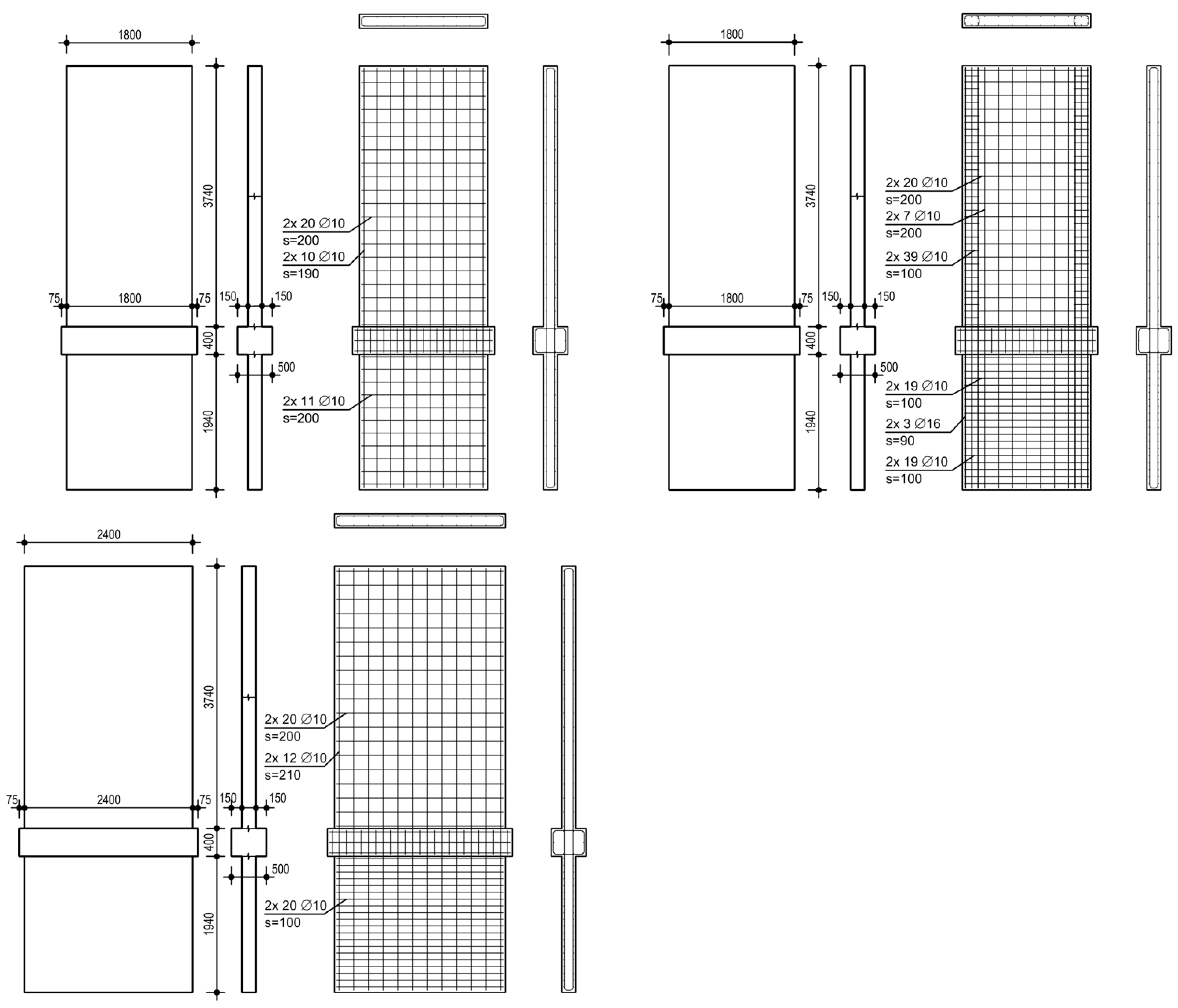
2.2. Shear Walls
- NW 1
- NW 2
- NW 3
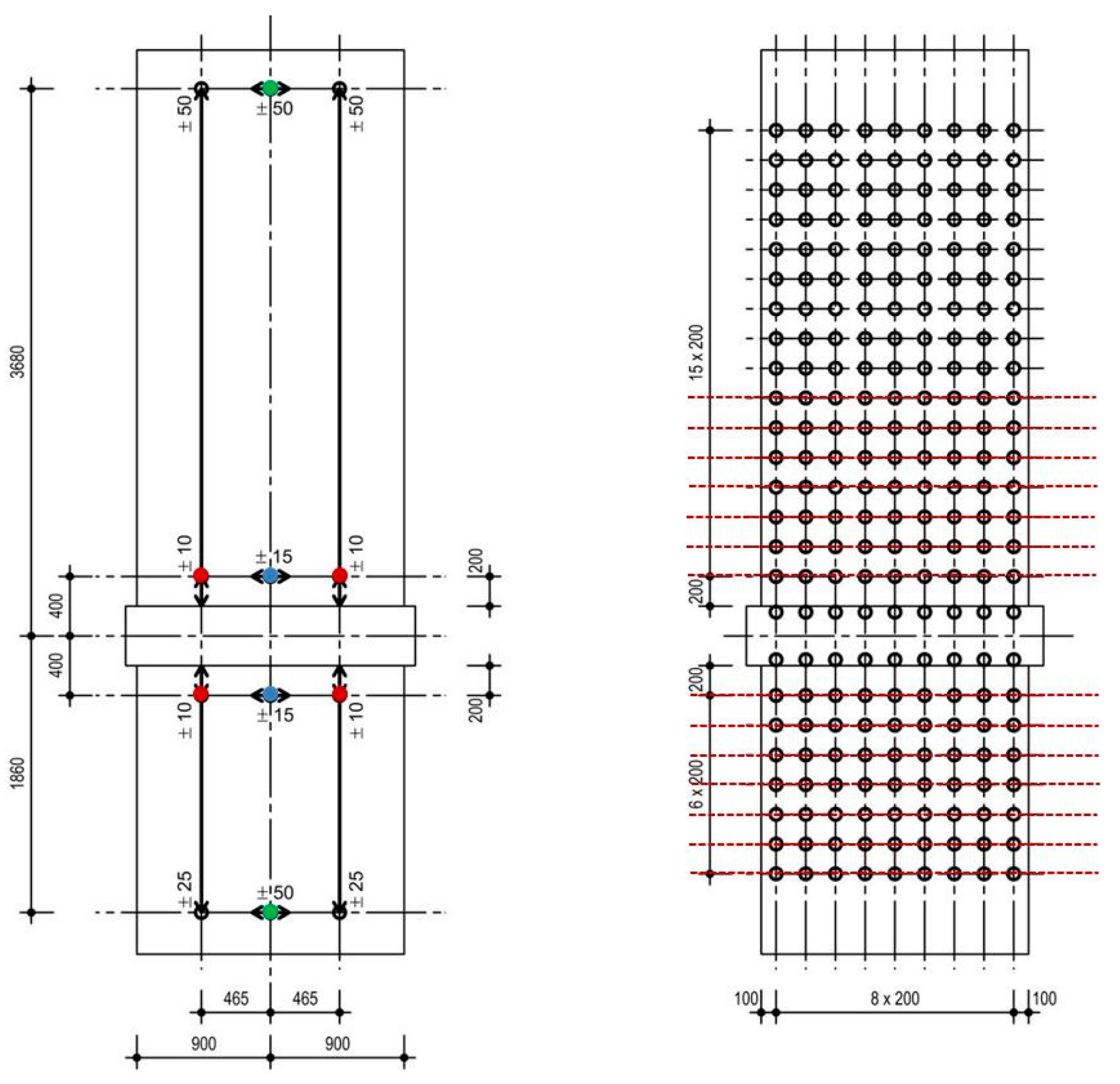
2.3. Measurement Technique
2.3.1. Measurement with Inductive Displacement Transducers (Back Side)
2.3.2. Optical Measurement (Front Side)
2.4. Loading Protocol
3. Results
3.1. NW 1
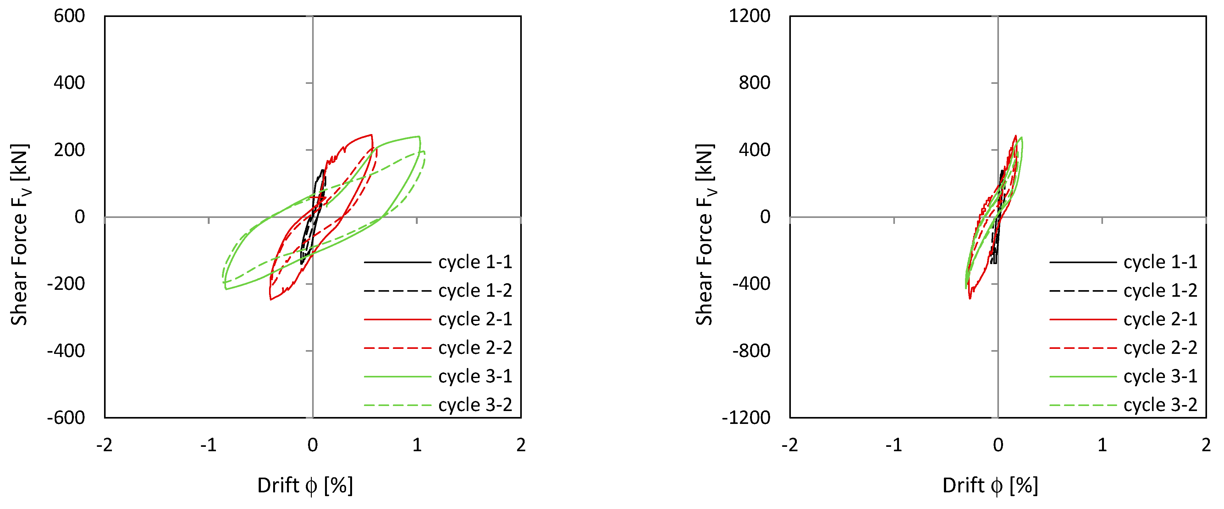
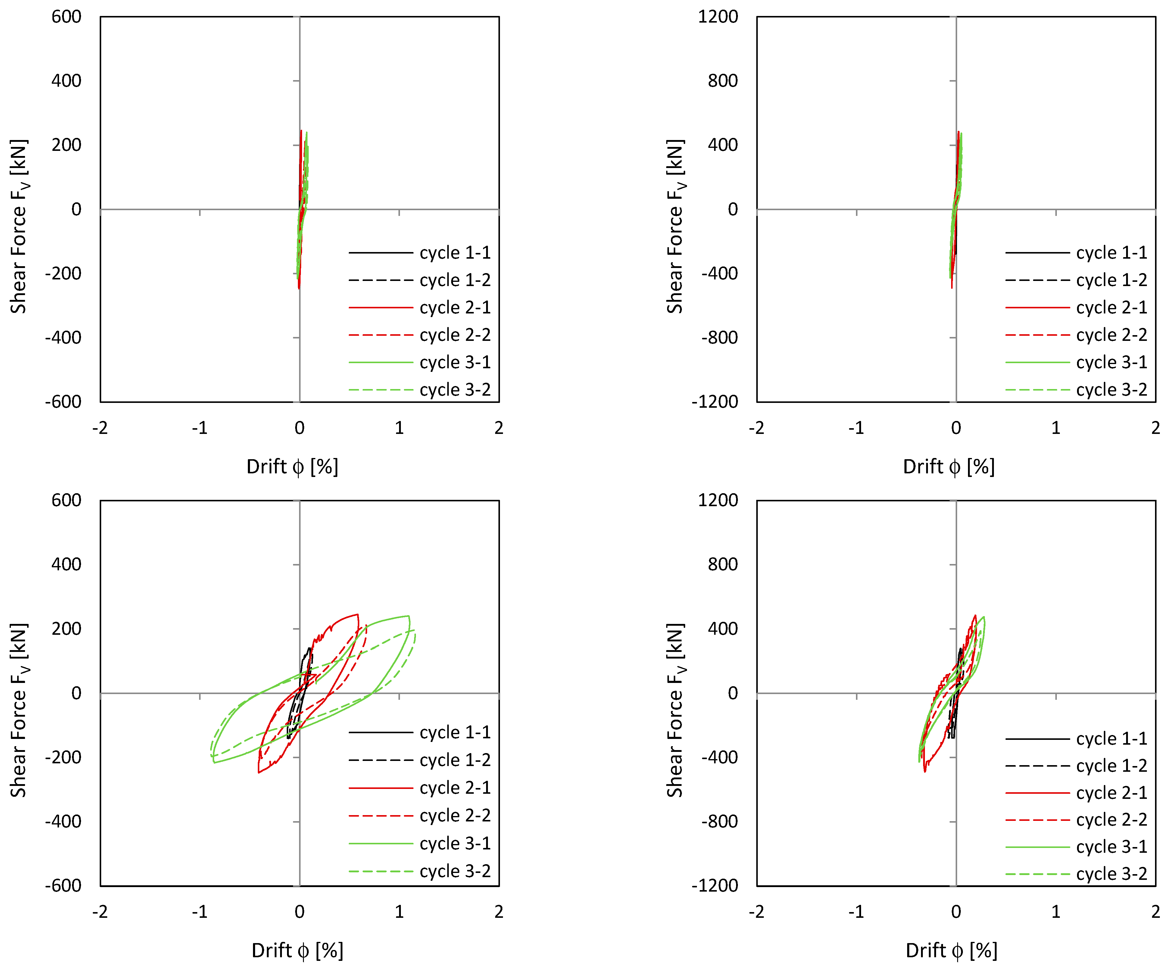
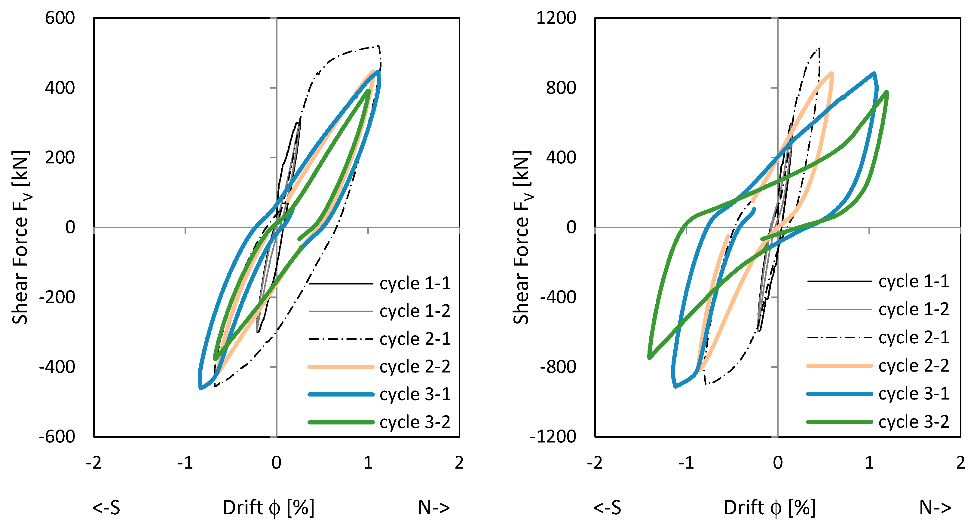
3.1.1. Load–Drift and Sliding Shear Behaviour
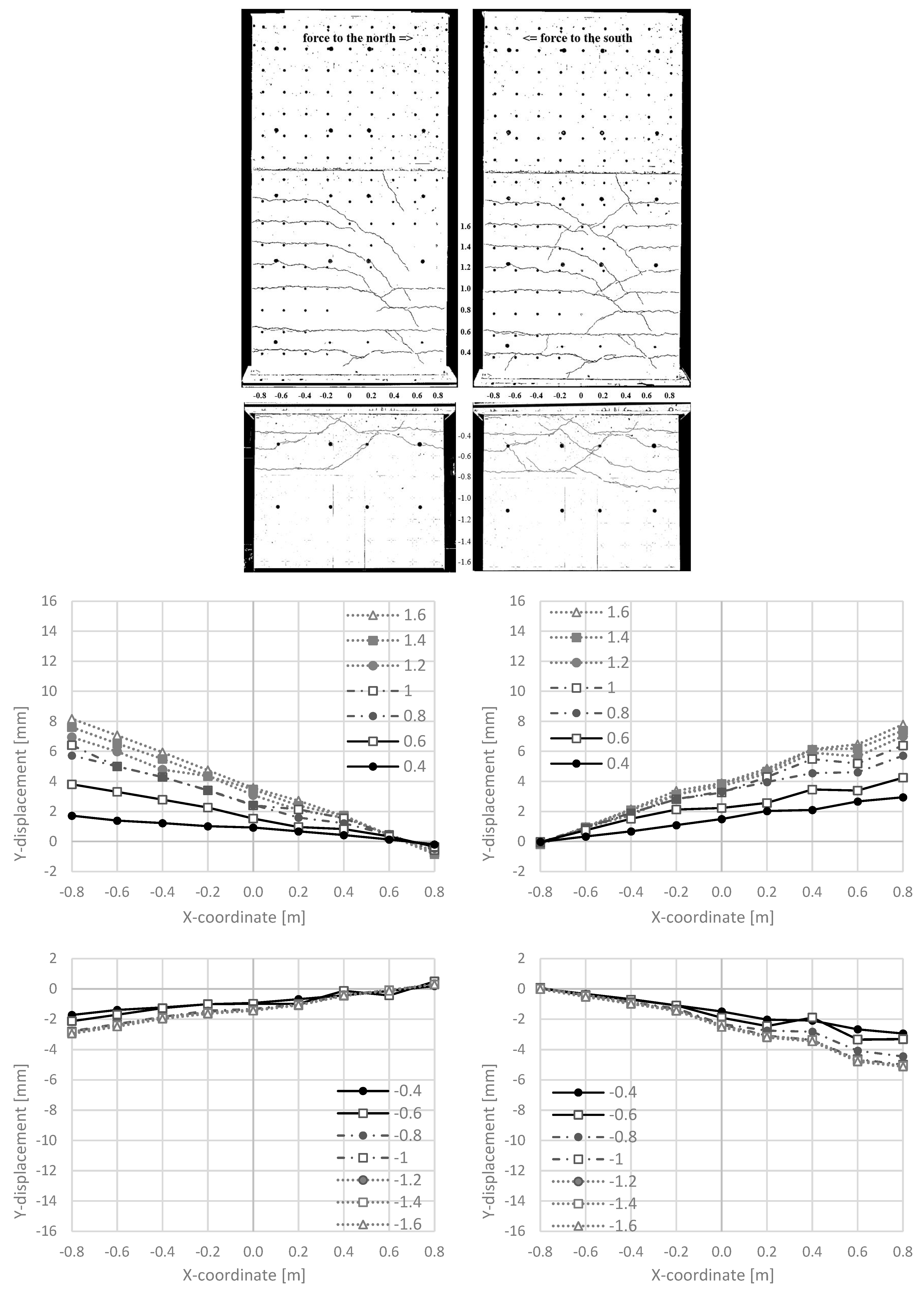
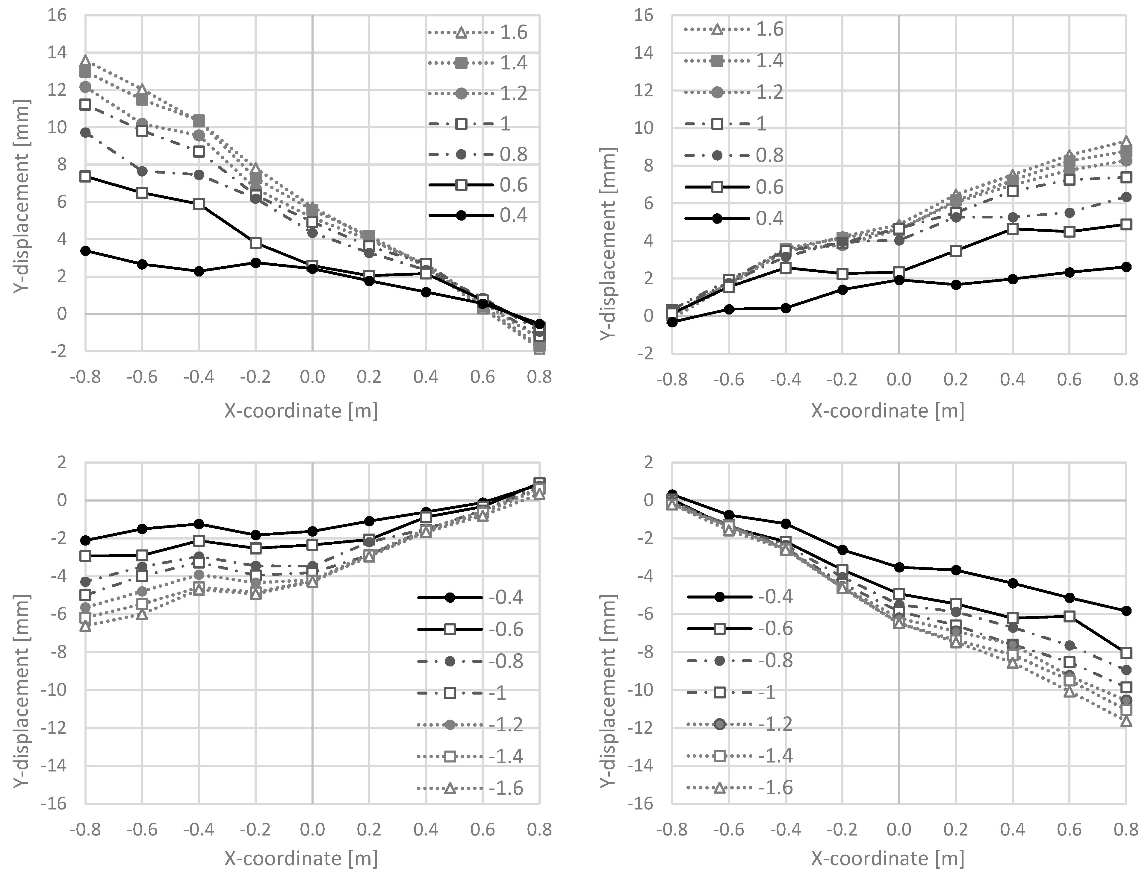
3.1.2. Cracking and Longitudinal Deformations around the Construction Joints
3.2. NW 2
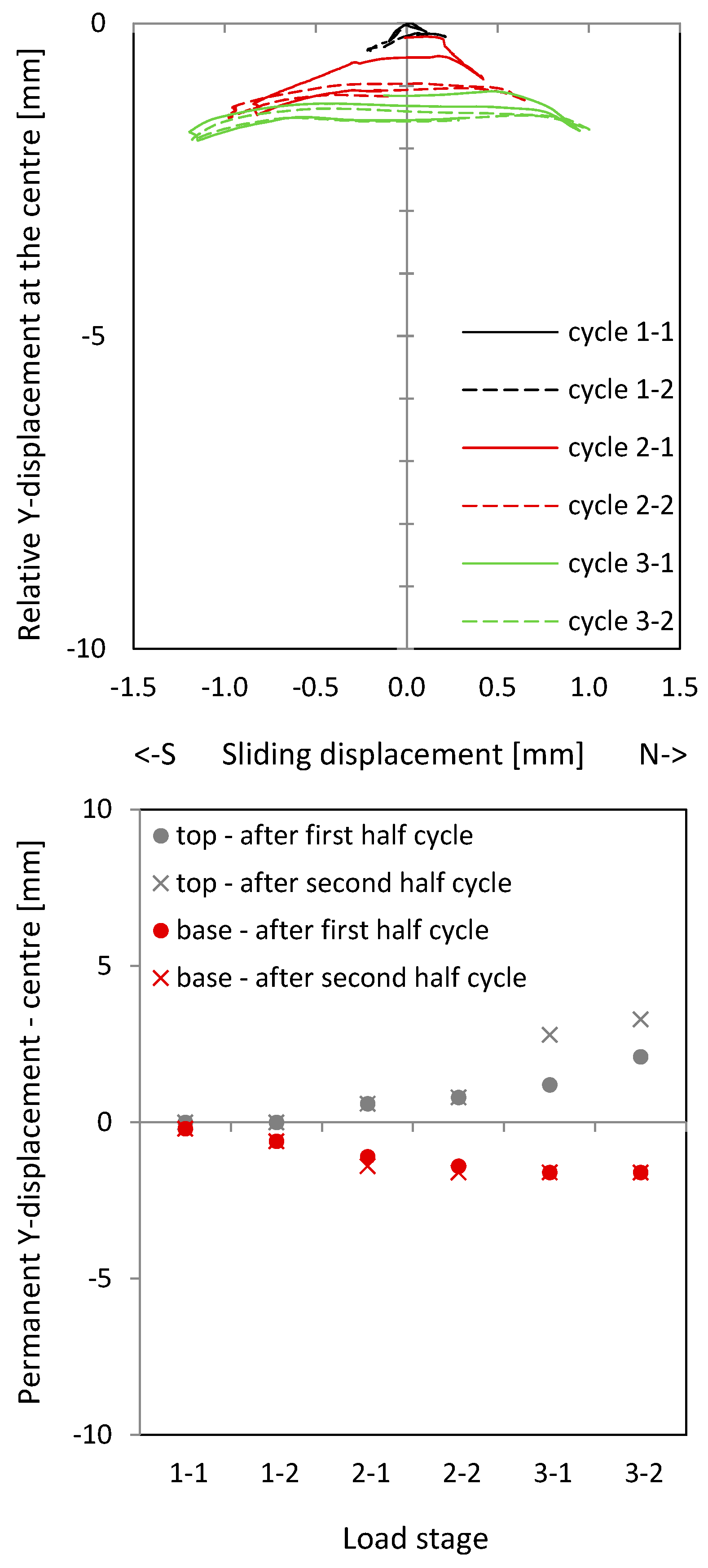
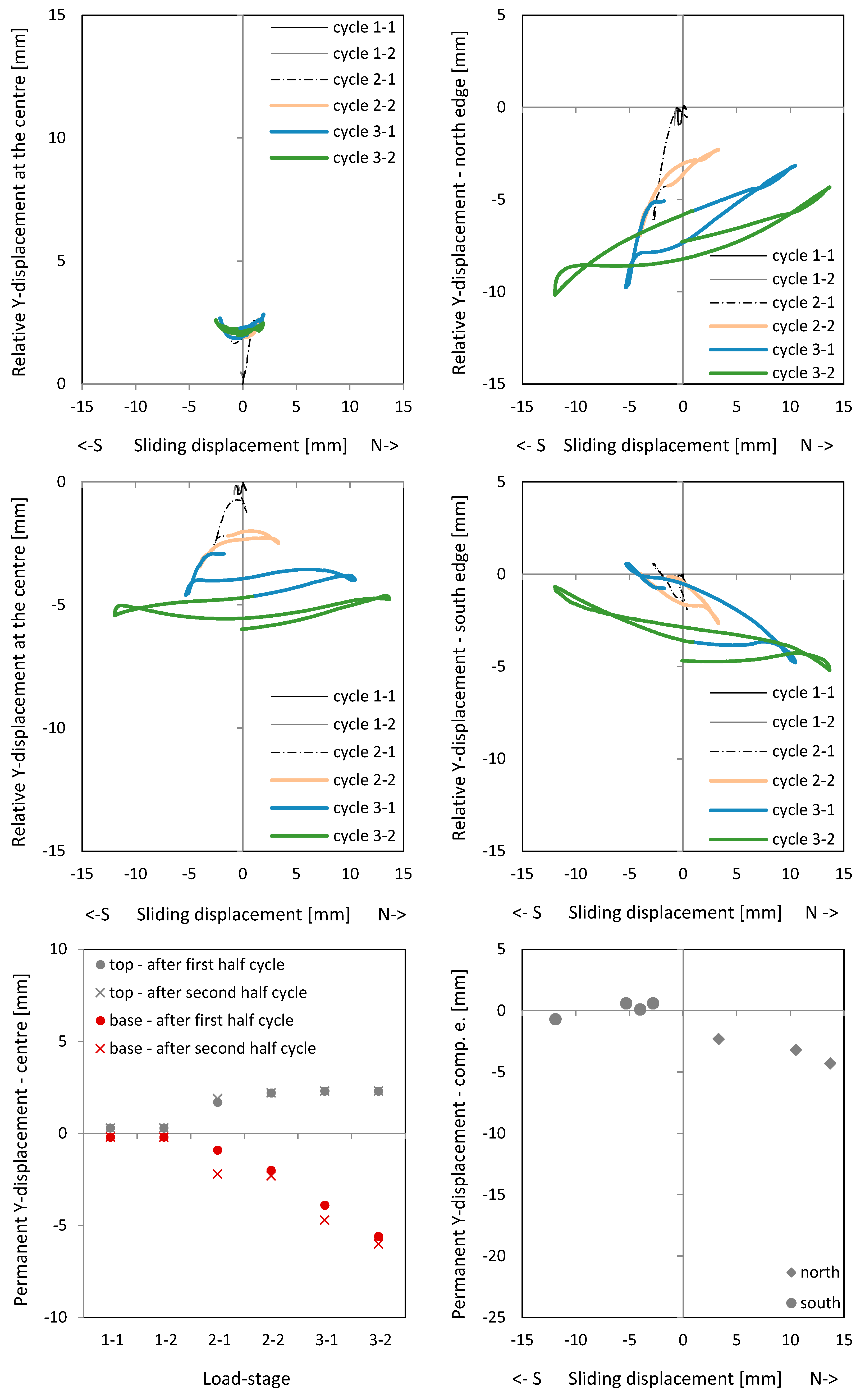
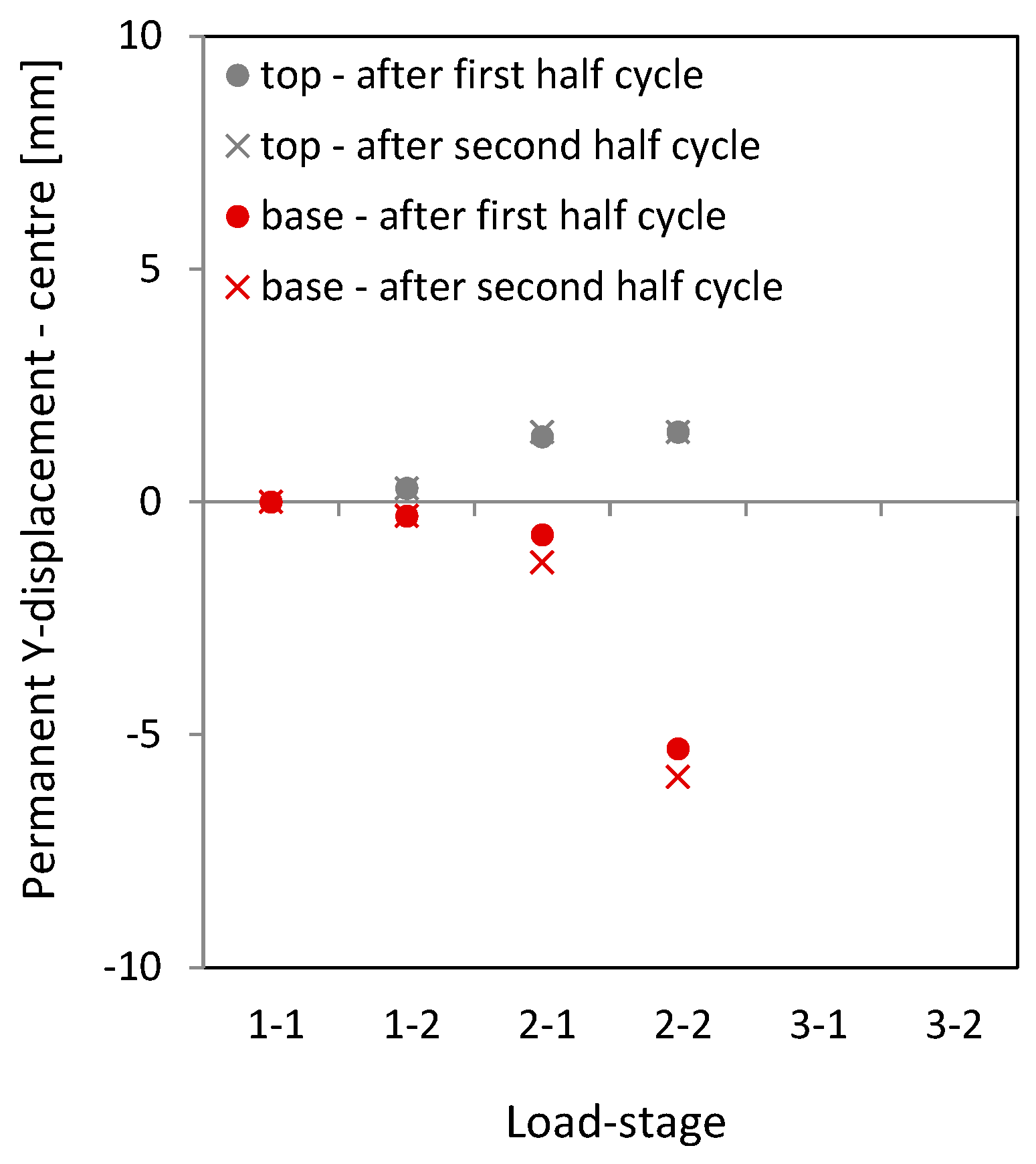
3.2.1. Load–Drift Behaviour, Sliding Shear and Longitudinal Displacements
3.2.2. Crack Pattern and Longitudinal Deformations
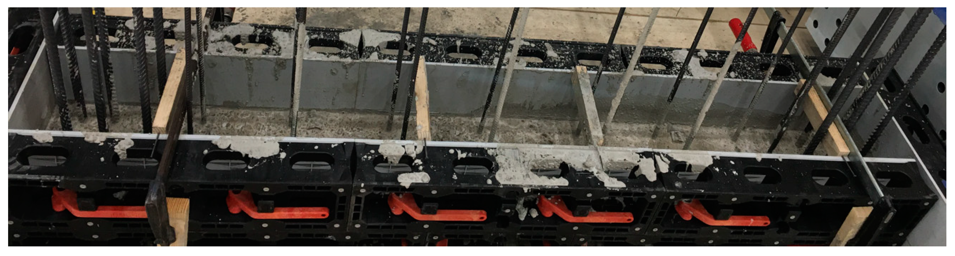
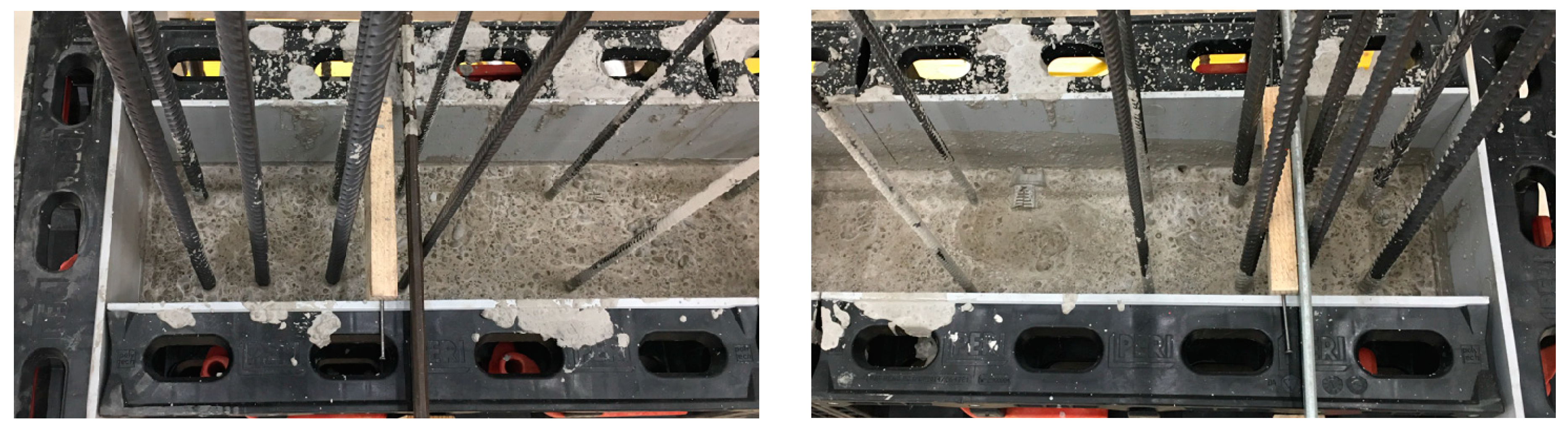
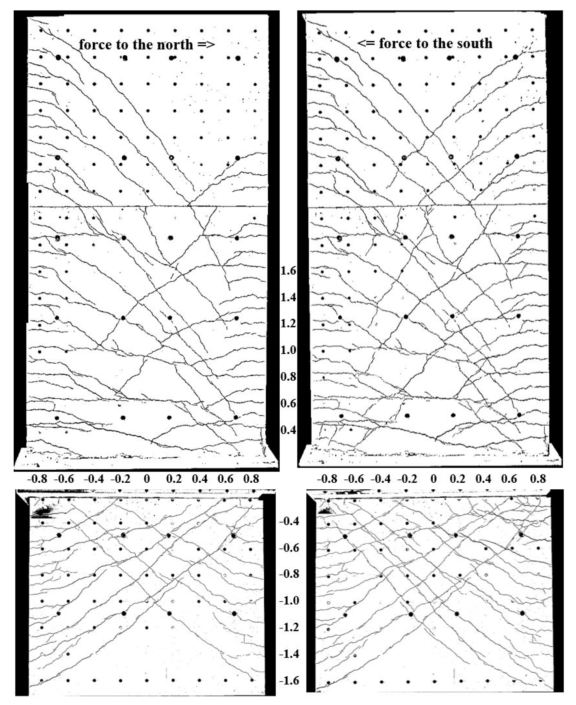
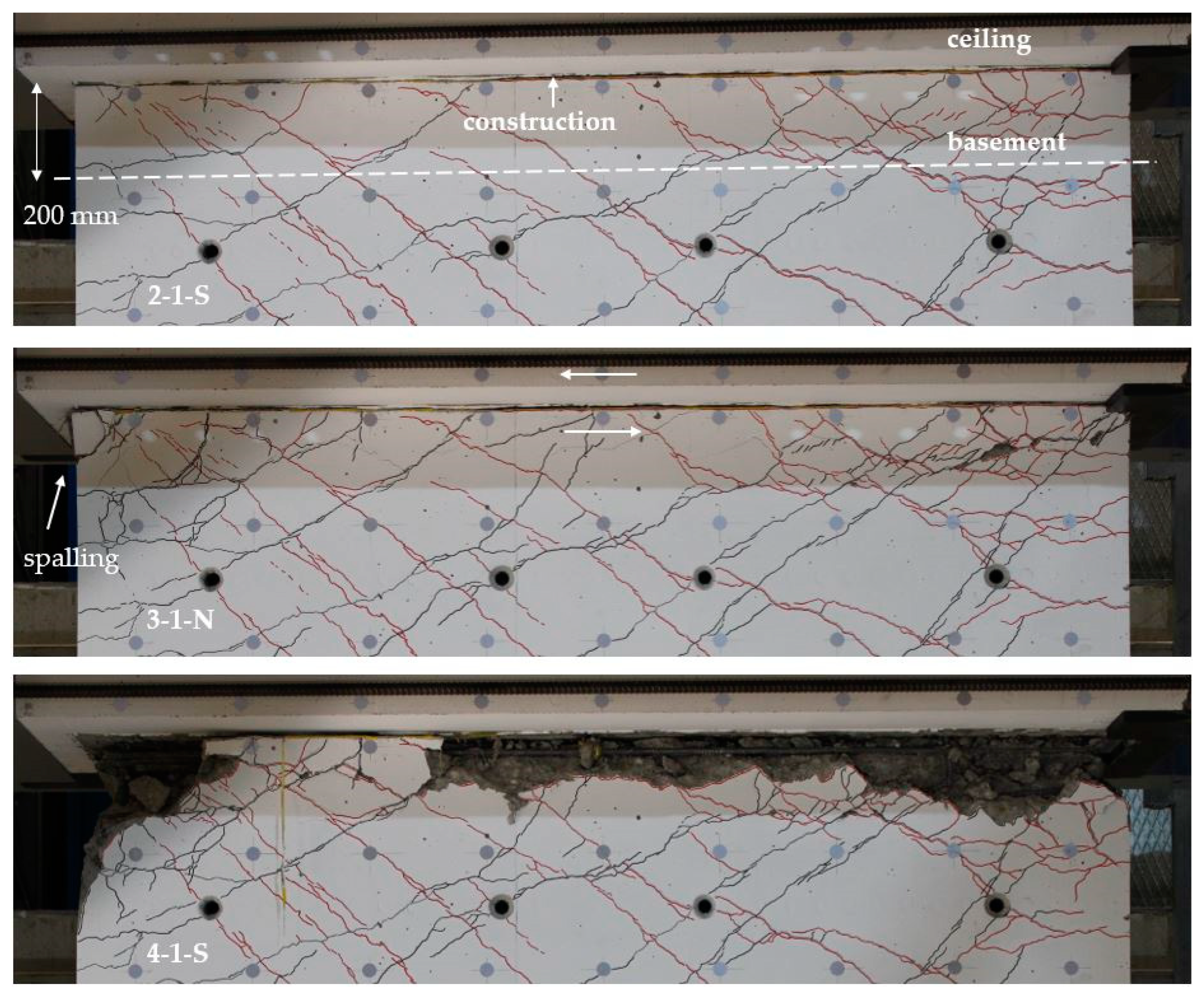
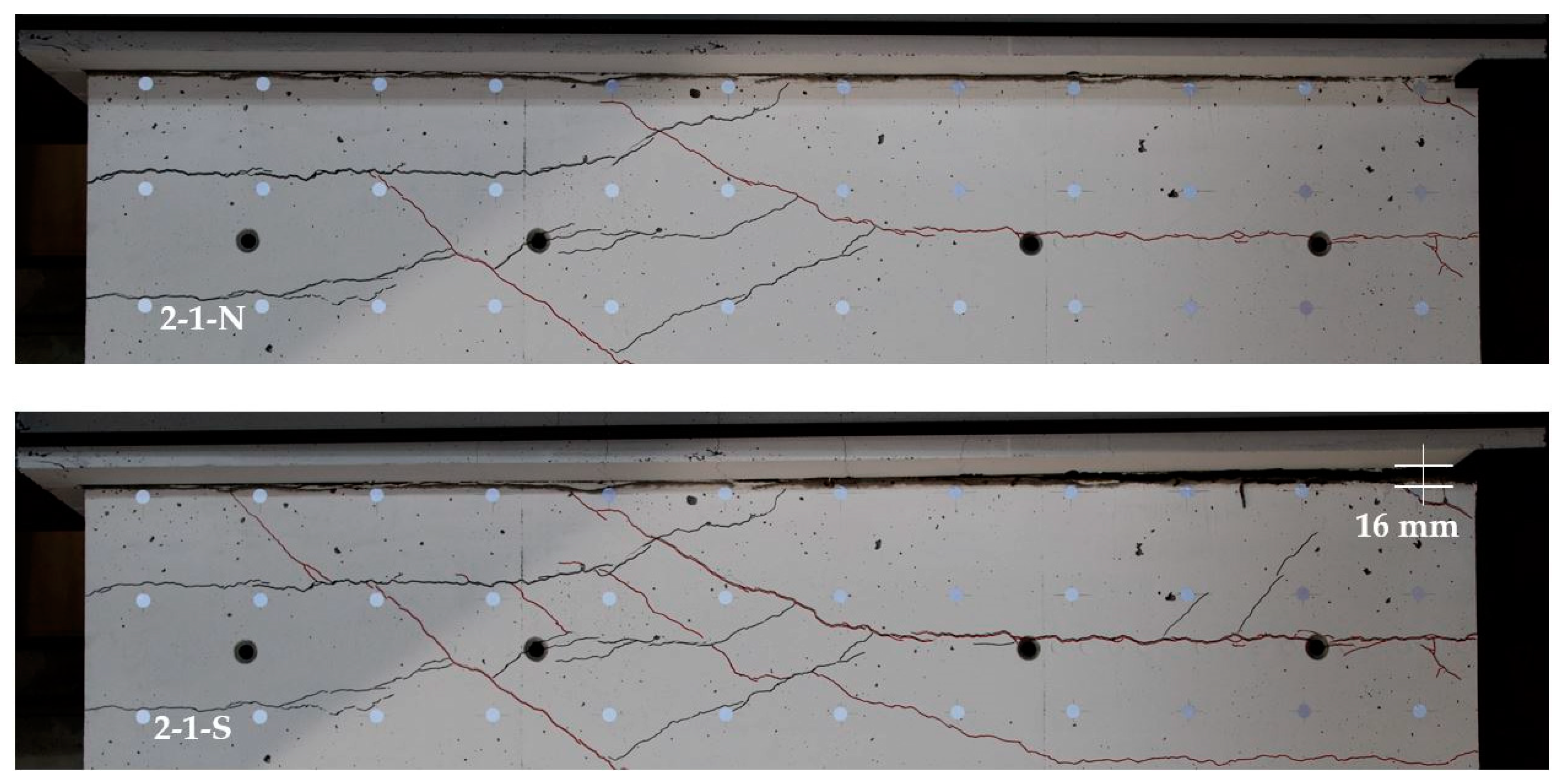
3.2.3. Photos of the Sliding Shear Zone
3.3. NW 3
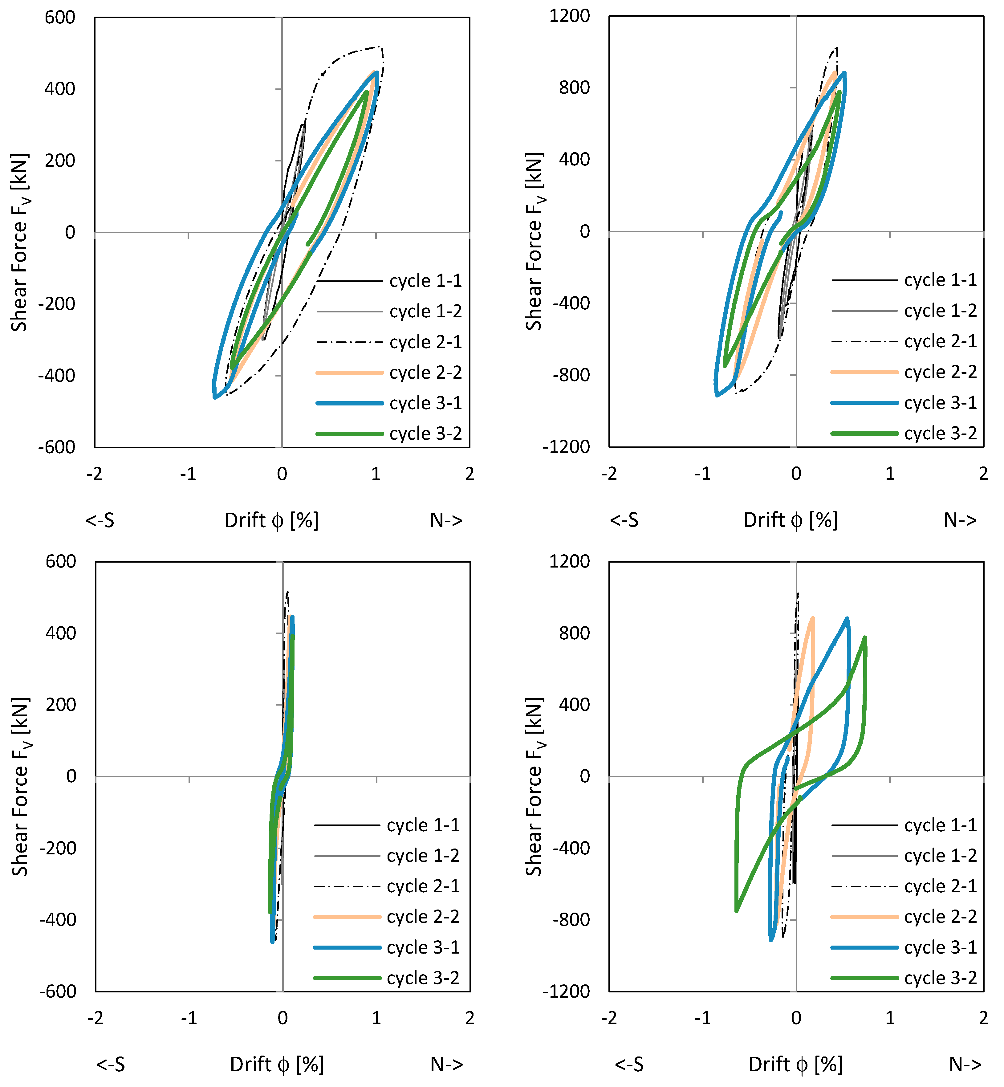
3.3.1. Load–Drift Behaviour, Sliding Shear and Longitudinal Displacements
3.3.2. Cracking and Longitudinal Deformations around the Construction Joints
3.3.3. Photos of the Sliding Shear Zone
4. Analysis
5. Conclusions
5.1. NW 1: Existing Wall, Slightly Reinforced/Aspect Ratio in the Clamped Part hw/lw~1
5.2. NW 2: New Construction Wall with Confined Boundaries and a Slightly Reinforced Web/Aspect Ratio in the Clamped Part hw/lw~1
5.3. NW 3: Existing Wall, Slightly Reinforced/Aspect Ratio in the Clamping Zone = hw/lw~0.78
5.4. Summary and Outlook
- Amount of reinforcement, which influences the compression resultant C.
- Distribution of the reinforcement (evenly distributed or concentrated in the edges), which influences the inner lever arm and, as a result, the compression resultant C.
- Axial force, which influences the compression resultant C.
Funding
Institutional Review Board Statement
Informed Consent Statement
Data Availability Statement
Conflicts of Interest
References
- Dazio, A.; Beyer, K.; Bachmann, H. Quasi-static cyclic tests and plastic hinge analysis of RC structural walls. Eng. Struct. 2009, 31, 1556–1571. [Google Scholar] [CrossRef]
- Dazio, A.; Wenk, T.; Bachmann, H. Versuche an Stahlbetontragwänden unter Zyklisch-Statischer Einwirkung (Tests on RC Walls under Cyclic-Static Action); IBK Report 239; Swiss Federal Institute of Technology ETH: Zürich, Switzerland, 1999. [Google Scholar]
- Hannewald, P.; Bimschas, M.; Dazio, A. Quasi-Static Cyclic Tests on RC Bridge Piers with Detailing Deficiencies; IBK Report 352; Swiss Federal Institute of Technology ETH: Zürich, Switzerland, 2013. [Google Scholar]
- Bimschas, M. Displacement-Based Seismic Assessment of Existing Bridges in Regions of Moderate Seismicity. Ph.D. Thesis, Swiss Federal Institute of Technology ETH, Zürich, Switzerland, 2010. [Google Scholar]
- Bimschas, M.; Chatzi, E.; Marti, P. Inelastic Deformation Analysis of Reinforced Concrete Bridge Piers, Part 1: Theory and Background. ACI Struct. J. 2015, 112, 267–276. [Google Scholar] [CrossRef]
- Bimschas, M.; Chatzi, E.; Marti, P. Inelastic Deformation Analysis of Reinforced Concrete Bridge Piers, Part 2: Application and Verification. ACI Struct. J. 2015, 112, 277–286. [Google Scholar] [CrossRef]
- Hannewald, P. Seismic Behavior of Poorly Detailed RC Bridge Piers. Ph.D. Thesis, Swiss Federal Institute of Technology EPFL, Lausanne, Switzerland, 2010. [Google Scholar]
- Hines, E.M.; Restrepo, J.I.; Seible, F. Force-displacement characterization of well-confined bridge piers. ACI Struct. J. 2004, 101, 537–548. [Google Scholar]
- Hoult, R.; Goldsworthy, H.; Lumantarna, E. Plastic Hinge Length for Lightly Reinforced Rectangular Concrete Walls. J. Earthq. Eng. 2018, 22, 1447–1478. [Google Scholar] [CrossRef]
- Schuler, H.; Meier, F.; Trost, B. Influence of the tension shift effect on the force–displacement curve of reinforced concrete shear walls. Eng. Struct. 2023, 274, 115144. [Google Scholar] [CrossRef]
- Trost, B. Interaction of Sliding, Shear and Flexure in the Seismic Response of Squat Reinforced Concrete Shear Walls. Ph.D. Thesis, ETH, Zürich, Switzerland, 2017. [Google Scholar]
- Synge, A.J. Ductility of Squat Shear Walls. In Research Report No. 80-8; Department of Civil Engineering, University of Canterbury: Christchurch, New Zealand, 1980. [Google Scholar]
- Paulay, T.; Priestley, M.J.N.; Synge, A.J. Ductility in Earthquake Resisting Squat Shear walls. ACI Struct. J. 1982, 101, 257–269. [Google Scholar]
- Luna, B.N.; Rivera, J.P.; Rocks, J.F.; Goksu, C.; Weinreber, S.; Whittaker, A.S. Low Aspect Ratio Rectangular Reinforced Concrete Shear Wall—Specimen SW8, Network for Earthquake Engineering Simulation (Distributor); University at Buffalo: Buffalo, NY, USA, 2013. [Google Scholar]
- Salonikios, T.N.; Kappos, A.J.; Tegos, I.A.; Penelis, G.G. Cyclic Load Behavior of Low-Slenderness Reinforced Concrete Walls: Design Basis and Test Results. ACI Struct. J. 1999, 96, 649–660. [Google Scholar]
- Schuler, H.; Trost, B. Sliding Shear Resistance of Squat Walls under Reverse Loading: Mechanical Model and Parametric Study. ACI Struct. J. 2016, 113, 711–721. [Google Scholar] [CrossRef]
- Trost, B.; Schuler, H.; Stojadinovic, B. Sliding in Compression Zones of Reinforced Concrete Shear Walls: Behavior and Modeling. ACI Struct. J. 2019, 116, 3–16. [Google Scholar] [CrossRef]
- Schuler, H. Flexural and Shear Deformation of Basement-Clamped Reinforced Concrete Shear Walls. Materials 2024, 17, 2267. [Google Scholar] [CrossRef] [PubMed]
- Park, R. Ductility Evaluation from Laboratory and Analytical Testing. In Proceedings of the Ninth World Conference on Earthquake Engineering, Tokyo-Kyoto, Japan, 2–9 August 1988; Volume VIII. [Google Scholar]


| Wall | hup | hbase = hw | t | lb1/2 | lweb | ρb1/2 | ρweb | ρV_up | ρV_base |
|---|---|---|---|---|---|---|---|---|---|
| [m] | [m] | [m] | [m] | [m] | [%] | [%] | [%] | [%] | |
| 1 | 3.68 | 1.86 | 0.20 | 0 | 1.80 | - | 0.44 | 0.39 | 0.39 |
| 2 | 3.68 | 1.86 | 0.20 | 0.27 | 1.26 | 2.23 | 0.44 | 0.39 | 0.79 |
| 4 | 3.68 | 1.86 | 0.20 | 0 | 2.40 | - | 0.39 | 0.39 | 0.79 |
| Wall | fc_cube_base | fc_cube_up | fst_base | fst_up |
|---|---|---|---|---|
| [MPa] | [MPa] | [MPa] | [MPa] | |
| 1 | 42.2 | 38.3 | 3.1 | 2.7 |
| 2 | 52.6 | 35.9 | 4.1 | 3.2 |
| 4 | 44.1 | 39.8 | 3.3 | 2.9 |
| Ø | Es | fsy | fsu | εy | εu |
|---|---|---|---|---|---|
| [GPa] | [MPa] | [MPa] | [mm/m] | [mm/m] | |
| 10 | 202 | 601 | 635 | 3.0 | 65.3 |
| 16 | 186 | 606 | 658 | 3.3 | 119 |
| Wall | Cycle | tw | x | z | FV | Τ = FV/(tw∙lw) | τx = FV/(tw∙x) | C = −FV∙hw/z | σx = C/(tw∙x) | τx/|σx| |
|---|---|---|---|---|---|---|---|---|---|---|
| [m] | [m] | [m] | [kN] | [MPa] | [MPa] | [kN] | [MPa] | [-] | ||
| NW 1 | 2-1 N | 0.2 | 0.16 | 0.98 | 485 | 1.3 | 15.2 | −822 | −25.7 | 0.59 |
| NW 2 | 2-1 N | 0.2 | 0.18 | 1.24 | 1135 | 3.2 | 31.5 | −1519 | −42.2 | 0.75 |
| NW 3 | 2-1 N | 0.2 | 0.19 | 1.29 | 750 | 2.1 | 19.7 | −965 | −25.4 | 0.78 |
| Wall | Cycle | ws | εs = ws/0.2 m | Κ = εs/(lw-0.1m-x) |
|---|---|---|---|---|
| [mm] | [mm/m] | [mrad/m] | ||
| NW 1 | 2-1 N | 1.7 | 8.5 | 5.5 |
| NW 2 | 2-1 N | 2.1 | 10.5 | 6.9 |
| NW 3 | 2-1 N | 4.0 | 20 | 9.5 |
Disclaimer/Publisher’s Note: The statements, opinions and data contained in all publications are solely those of the individual author(s) and contributor(s) and not of MDPI and/or the editor(s). MDPI and/or the editor(s) disclaim responsibility for any injury to people or property resulting from any ideas, methods, instructions or products referred to in the content. |
© 2024 by the author. Licensee MDPI, Basel, Switzerland. This article is an open access article distributed under the terms and conditions of the Creative Commons Attribution (CC BY) license (https://creativecommons.org/licenses/by/4.0/).
Share and Cite
Schuler, H. Sliding Shear Failure of Basement-Clamped Reinforced Concrete Shear Walls. Materials 2024, 17, 4111. https://doi.org/10.3390/ma17164111
Schuler H. Sliding Shear Failure of Basement-Clamped Reinforced Concrete Shear Walls. Materials. 2024; 17(16):4111. https://doi.org/10.3390/ma17164111
Chicago/Turabian StyleSchuler, Harald. 2024. "Sliding Shear Failure of Basement-Clamped Reinforced Concrete Shear Walls" Materials 17, no. 16: 4111. https://doi.org/10.3390/ma17164111
APA StyleSchuler, H. (2024). Sliding Shear Failure of Basement-Clamped Reinforced Concrete Shear Walls. Materials, 17(16), 4111. https://doi.org/10.3390/ma17164111