A Hybrid Method Combining Voronoi Diagrams and the Random Walk Algorithm for Generating the Mesostructure of Concrete


Abstract
1. Introduction
- (1)
- The “take-and-place” method [1,2,3] involves randomly depositing aggregates into the target domain and then conducting intersection checks to retain aggregates meeting the specified criteria. Although this method ensures rational aggregate grading, it may fall short of achieving a high aggregate volume fraction. For instance, Zhang et al. [4] utilized X-ray computed tomography (XCT) to scan aggregates and employed the take-and-place algorithm to establish mesoscale concrete models.
- (2)
- The “place-and-generate” method [5,6] requires randomly distributed points to be generated within the target domain, and subsequently, various types of aggregates are generated at these points using aggregate growth algorithms [5,7] or Voronoi diagrams [8,9,10]. Although a high aggregate volume fraction can be achieved, the aggregate grading always deviates from the ideal curve.
- (3)
- The “random walk algorithm” (RWA) [11,12] involves sequentially introducing generated aggregate particles into the target domain through a random walk process, including translations and rotations until no more aggregates can be placed. Although the aggregate volume fraction and grading can be ensured, it exhibits a low efficiency in placing polyhedral aggregates. Wu et al. [13] employed the RWA to obtain a mesoscopic model of concrete with convex polyhedra.
- (4)
- The “aggregate packing” method [14] generates aggregates individually and arranges them layer by layer into the domain. While no intersection or overlapping check is required, it may result in a lower aggregate volume fraction due to the presence of gaps between aggregates, and once aggregates are generated by the algorithm, they cannot be moved anymore. Huang et al. [15] utilized XCT to scan real aggregates and employed the aggregate packing algorithm to generate realistic mesoscale concrete models. Liang et al. [16] combined the aggregate packing and take-and-place algorithms to introduce “partial aggregates” into the target domain and established a two-dimensional mesoscopic model for asphalt concrete.
2. Voronoi–Random Walk Aggregate Generation Method
2.1. Polyhedral Aggregate Generation
2.1.1. Random Walk Algorithm (RWA)
2.1.2. Voronoi Polyhedra Generation Algorithm
- (1)
- Generate spherical aggregates according to the user-defined grading curve.
- (2)
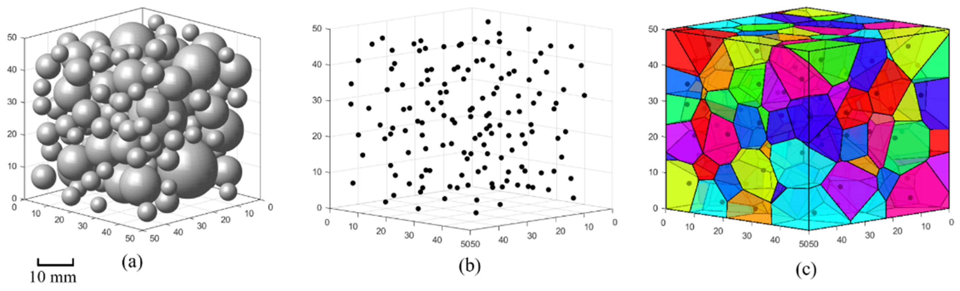
- Employ the RWA to place spherical aggregates into the target domain, as shown in Figure 1a.
- (3)
- Take the centers of the spherical aggregates as seed points for the Voronoi tessellation, as shown in Figure 1b.
- (4)
- Employ the Delaunay triangulation to generate Voronoi polyhedra representing the aggregates based on the generated seed points, as illustrated in Figure 1c.
2.2. Polyhedral Geometry Optimization
2.2.1. Eliminating Short Edges
2.2.2. Improving Sharp Angles
- (1)
- Randomly select a polyhedron Vi(Pi, Si) and a vertex Pi(Pi1, Pi2, …, Pik), where k represents the number of vertices.
- (2)
- Calculate the distance Dij from the seed point to the vertices:
- (3)
- Find the minimum distance Dmin = min(d(Pij, Si)).
- (4)
- Calculate the distance Dij′ from the seed point to the new vertices using the following expression:
- (5)
- Perform non-uniform scaling down on the polyhedron, with the coordinates of the new vertices denoted as Pi′(Pi1′, Pi2′, …, Pik′):
2.3. Adjustment of Aggregate Grading
2.3.1. Aggregate Grading
2.3.2. Range Mapping Algorithm
- (1)
- For a polyhedron Vi(Pi, Si) with j vertices, calculate the distance d(Pim, Pin) (m ≠ n; m, n = 1, 2, 3, …, j) between any two vertices Pim and Pin. The maximum distance is taken as the particle size of the polyhedron and denoted as d(Vi) = max(d(Pim, Pin)).
- (2)
- Sort the polyhedra by particle size from small to large and range the Voronoi polyhedra collection based on the number of polyhedra in each sub-range, which is calculated as follows:
- (3)
- Map [Di,1, Di,2] to [di, di+1]. Ds represents the size of the polyhedron in the particle size range [Di,1, Di,2]. Any Ds can be used to find the corresponding value ds in [di, di+1] according to
- (4)
- Scale the polyhedral uniformly. The original vertex Pi of a specific polyhedron moves toward the seed point Si, and the coordinates of the new vertex Pi′ are calculated according to a scaling factor qs, which is determined by
2.4. Comparison with Fuller’s Curve
2.5. Flowchart of the V-RW Algorithm
3. Numerical Simulations
3.1. Mesoscale Model of Aggregate
3.2. Finite Element Modeling
3.3. Simulation Results and Discussion
4. Discussion
4.1. Efficiency of the V-RW Algorithm
4.2. Polyhedral Reshaping Parameter
4.3. Aggregate Gradation
4.3.1. Grading Type
4.3.2. Range Number in the Range Mapping Algorithm
5. Conclusions
- (1)
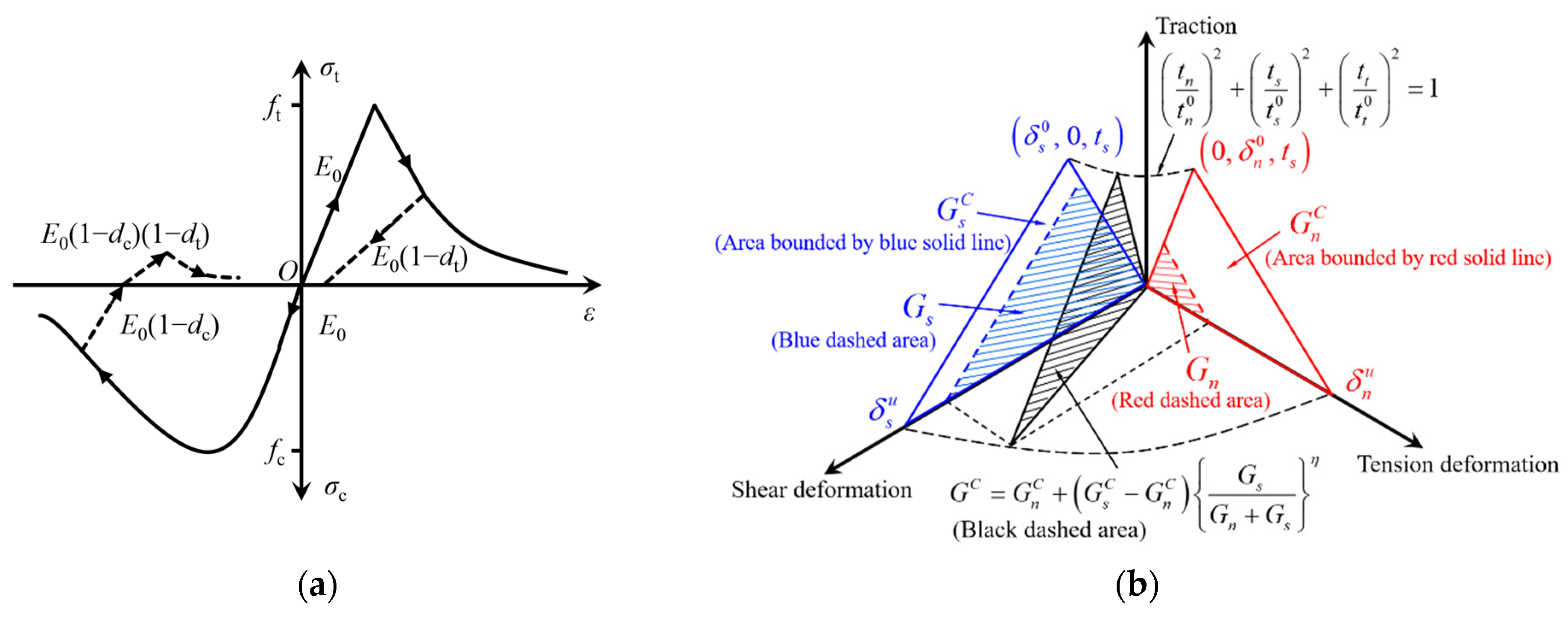
- In the proposed method, the random walk algorithm was used to place seed points, which were then used to generate Voronoi polyhedra. The geometric shapes of these polyhedra were optimized through short-edge elimination and sharp-angle improvement. A range mapping algorithm is employed to obtain aggregate models that meet the grading requirements. In the simulations performed in this study, tetrahedral meshing was used to discretize aggregates and mortar, a cohesive element with zero thickness was used to simulate the ITZ, the concrete damaged plasticity model was used to simulate the damage in mortar, and a 3D mesostructure model of concrete was established.
- (2)
- The grading of the aggregates affected the alignment with the Fuller curve. The generated four-level grading aggregate model aligned well with the Fuller curve. The polyhedral reshaping parameter β affected the aggregate volume fraction. Increasing β could improve the volume fraction. Changes in β had little effect on the aggregate grading curve. The range mapping algorithm could significantly improve the aggregate volume fraction as well, but too many or too few ranges could cause the grading curve to deviate from the Fuller curve. A four-range mapping could achieve a reasonable grading and a high aggregate volume fraction.
- (3)
- The present algorithm has the following limitations: The generated aggregate particles all retain “convex” shapes, which do not align with the actual shapes of some aggregates with defects, particularly those with “flaky” and “needle-like” morphologies. During concrete damage, cracks tend to initiate and propagate from these defective aggregates due to stress concentration effects. Consequently, exploring the generation of aggregates with defective characteristics and conducting corresponding numerical simulations for validation have emerged as crucial directions for future research. On the other hand, in the current algorithm, the positions of all aggregate particles relative to their seed points remain fixed, which restricts the further increase in aggregate volume fraction to a certain extent. To address this issue, a potential research approach involves applying microrotations and translations to the aggregate particles, followed by the secondary generation of fine aggregate particles based on the adjusted coarse aggregates, aiming to generate aggregate models with higher volume fractions. Lastly, and most importantly, effectively extending the concrete mesoscale model to practical engineering applications poses a challenge. Integrating mesoscale models at the component level often leads to extremely large computational demands and high costs. Therefore, investigating the application of the proposed algorithm in numerical simulations of large-scale components has become a significant direction for future research.
- (4)
- The V-RW algorithm showed a significant advantage of efficiently generating polyhedral aggregates with random shapes and specific grading models. Broadly, the V-RW method could also be used to simulate the mesostructures of other particle-filled composite materials, as well as the mesostructure of concrete composed of real aggregates. Examples of composite materials that consist of irregular polyhedral aggregates include crushed lightweight aggregate concrete, asphalt aggregate concrete, and coral lightweight aggregate concrete. Based on the established 3D mesostructure of concrete, finite element simulations can be used to study macroscopic mechanical properties and mesoscale mechanical behavior. With these advantages, the V-RW method provided an efficient and accurate tool for numerical simulations of concrete with real aggregates.
Author Contributions
Funding
Institutional Review Board Statement
Informed Consent Statement
Data Availability Statement
Conflicts of Interest
Nomenclature
| N | Number of Voronoi seeds |
| Si | Coordinates of seed point |
| Pi | Set of vertex coordinates of the ith Voronoi polyhedron |
| Vi | Points set of the ith Voronoi polyhedron |
| Dij | Distance between Si and Pij |
| Dmin | Minimum distance between Si and Pij |
| β | Polyhedral reshaping parameter |
| Pi′ | Coordinates of the new vertices |
| q | Scaling factor |
| d | Aperture of the sieve |
| P(d) | Cumulative percentage passing the sieve |
| dmax | Maximum size of the aggregate particles |
| n | A constant parameter |
| Vagg | Volume of fraction of aggregates |
| di,i+1 | Representative size of the grading range |
| Q | Quantity percentage of the grading range |
| Npoly | Number of Voronoi polyhedra |
| Di,1 | Minimum particle size of the ith range |
| Di,2 | Maximum particle size of the ith range |
| Ds | Size of the polyhedron aggregate |
| G | Grading type |
| P | Range types |
References
- Wang, Z.M.; Kwan, A.K.H.; Chan, H.C. Mesoscopic Study of Concrete I: Generation of Random Aggregate Structure and Finite Element Mesh. Comput. Struct. 1999, 70, 533–544. [Google Scholar] [CrossRef]
- Wriggers, P.; Moftah, S.O. Mesoscale Models for Concrete: Homogenisation and Damage Behaviour. Finite Elem. Anal. Des. 2006, 42, 623–636. [Google Scholar] [CrossRef]
- Wang, X.F.; Yang, Z.J.; Yates, J.R.; Jivkov, A.P.; Zhang, C. Monte Carlo Simulations of Mesoscale Fracture Modelling of Concrete with Random Aggregates and Pores. Constr. Build. Mater. 2015, 75, 35–45. [Google Scholar] [CrossRef]
- Zhang, L.; Sun, X.; Xie, H.; Feng, J. Three-Dimensional Mesoscale Modeling and Failure Mechanism of Concrete with Four-Phase. J. Build. Eng. 2023, 64, 105693. [Google Scholar] [CrossRef]
- Gao, Z.; Liu, G. Two-dimensional random aggregate structure for concrete. J. Tsinghua Univ. (Sci. Technol.) 2003, 43, 710–714. [Google Scholar] [CrossRef]
- Stankowski, T. Numerical Simulation of Failure in Particle Composites. Comput. Struct. 1992, 44, 459–468. [Google Scholar] [CrossRef]
- Liu, G.; Gao, Z. Random 3-D aggregate structure for concrete. J. Tsinghua Univ. (Sci. Technol.) 2003, 43, 1120–1123. [Google Scholar] [CrossRef]
- Caballero, A.; López, C.M.; Carol, I. 3D Meso-Structural Analysis of Concrete Specimens under Uniaxial Tension. Comput. Methods Appl. Mech. Eng. 2006, 195, 7182–7195. [Google Scholar] [CrossRef]
- De Schutter, G.; Taerwe, L. Random Particle Model for Concrete Based on Delaunay Triangulation. Mater. Struct. 1993, 26, 67–73. [Google Scholar] [CrossRef]
- Li, C.; Song, X. Mesoscale Modeling of Chloride Transport in Unsaturated Concrete Based on Voronoi Tessellation. Cem. Concr. Res. 2022, 161, 106932. [Google Scholar] [CrossRef]
- Song, X. Application of Random Walking in Concrete Sphere Aggregates Simulation. J. Ningbo Univ. Nat. Sci. Eng. Ed. 2010, 23, 104–108. [Google Scholar] [CrossRef]
- Zhang, Z.; Song, X.; Liu, Y.; Wu, D.; Song, C. Three-Dimensional Mesoscale Modelling of Concrete Composites by Using Random Walking Algorithm. Compos. Sci. Technol. 2017, 149, 235–245. [Google Scholar] [CrossRef]
- Wu, Z.; Yu, H.; Zhang, J.; Ma, H. Mesoscopic Study of the Mechanical Properties of Coral Aggregate Concrete under Complex Loads. Compos. Struct. 2023, 308, 116712. [Google Scholar] [CrossRef]
- Tang, X.; Zhang, C.; Shi, J. A Multiphase Mesostructure Mechanics Approach to the Study of the Fracture-Damage Behavior of Concrete. Sci. China (Ser. E Technol. Sci.) 2008, 51, 8–24. [Google Scholar] [CrossRef]
- Huang, Y.; Guo, F.; Zhang, H.; Yang, Z. An Efficient Computational Framework for Generating Realistic 3D Mesoscale Concrete Models Using Micro X-Ray Computed Tomography Images and Dynamic Physics Engine. Cem. Concr. Compos. 2022, 126, 104347. [Google Scholar] [CrossRef]
- Liang, S.; Liao, M.; Tu, C.; Luo, R. Fabricating and Determining Representative Volume Elements of Two-Dimensional Random Aggregate Numerical Model for Asphalt Concrete without Damage. Constr. Build. Mater. 2022, 357, 129339. [Google Scholar] [CrossRef]
- Zhang, J.; Wang, Z.; Yang, H.; Wang, Z.; Shu, X. 3D Meso-Scale Modeling of Reinforcement Concrete with High Volume Fraction of Randomly Distributed Aggregates. Constr. Build. Mater. 2018, 164, 350–361. [Google Scholar] [CrossRef]
- Zhang, J.; Yang, H.; Zhang, Y.; Wang, Z.; Wang, Z.; Shu, X. Numerical Investigations on the Effect of Reinforcement on Penetration Resistance of Concrete Slabs Using a 3D Meso-Scale Method. Constr. Build. Mater. 2018, 188, 793–808. [Google Scholar] [CrossRef]
- Ren, H.; Rong, Y.; Xu, X. Mesoscale Investigation on Failure Behavior of Reinforced Concrete Slab Subjected to Projectile Impact. Eng. Fail. Anal. 2021, 127, 105566. [Google Scholar] [CrossRef]
- Naderi, S.; Tu, W.; Zhang, M. Meso-Scale Modelling of Compressive Fracture in Concrete with Irregularly Shaped Aggregates. Cem. Concr. Res. 2021, 140, 106317. [Google Scholar] [CrossRef]
- Zhang, H.; Xu, C.; Zhou, Y.; Shu, J.; Huang, K. Hybrid Phase-Field Modeling of Mesoscopic Failure in Concrete Combined with Fourier-Voronoi Stochastic Aggregate Distribution Modelling Approach. Constr. Build. Mater. 2023, 394, 132106. [Google Scholar] [CrossRef]
- Ma, D.; Liu, C.; Zhu, H.; Liu, Y.; Jiang, Z.; Liu, Z.; Zhou, L.; Tang, L. High Fidelity 3D Mesoscale Modeling of Concrete with Ultrahigh Volume Fraction of Irregular Shaped Aggregate. Compos. Struct. 2022, 291, 115600. [Google Scholar] [CrossRef]
- Wei, X.; Sun, Y.; Gong, H.; Li, Y.; Chen, J. Repartitioning-Based Aggregate Generation Method for Fast Modeling 3D Mesostructure of Asphalt Concrete. Comput. Struct. 2023, 281, 107010. [Google Scholar] [CrossRef]
- Cavalline, T.L.; Castrodale, R.W.; Freeman, C.; Wall, J. Impact of Lightweight Aggregate on Concrete Thermal Properties. ACI Mater. J. 2017, 114, 945–956. [Google Scholar] [CrossRef]
- Chen, Y.; Feng, J.; Li, H.; Meng, Z. Effect of Coarse Aggregate Volume Fraction on Mode II Fracture Toughness of Concrete. Eng. Fract. Mech. 2021, 242, 107472. [Google Scholar] [CrossRef]
- Du, Q.; Gunzburger, M. Grid Generation and Optimization Based on Centroidal Voronoi Tessellations. Appl. Math. Comput. 2002, 133, 591–607. [Google Scholar] [CrossRef]
- Xu, L.; Yang, H.; Hu, J.; Lu, G.; Wang, Z. 3D random aggregate model of concrete based on Voronoi method. J. Build. Struct. 2015, 36, 325–332. [Google Scholar] [CrossRef]
- Naderi, S.; Zhang, M. An Integrated Framework for Modelling Virtual 3D Irregulate Particulate Mesostructure. Powder Technol. 2019, 355, 808–819. [Google Scholar] [CrossRef]
- Zhang, Y.; Wang, Z.; Zhang, J.; Zhou, F.; Wang, Z.; Li, Z. Validation and Investigation on the Mechanical Behavior of Concrete Using a Novel 3D Mesoscale Method. Materials 2019, 12, 2647. [Google Scholar] [CrossRef]
- Fuller, W.B.; Thompson, S.E. The Laws of Proportioning Concrete. Trans. Am. Soc. Civ. Eng. 1907, 59, 67–143. [Google Scholar] [CrossRef]
- Xiong, X.; Xiao, Q. Meso-Scale Simulation of Concrete Based on Fracture and Interaction Behavior. Appl. Sci. 2019, 9, 2986. [Google Scholar] [CrossRef]
- Zhou, G.; Xu, Z. 3D Mesoscale Investigation on the Compressive Fracture of Concrete with Different Aggregate Shapes and Interface Transition Zones. Constr. Build. Mater. 2023, 393, 132111. [Google Scholar] [CrossRef]
- Du, X.; Jin, L.; Ma, G. Numerical Simulation of Dynamic Tensile-Failure of Concrete at Meso-Scale. Int. J. Impact Eng. 2014, 66, 5–17. [Google Scholar] [CrossRef]
- GB 50010-2010; Code for Design of Concrete Structures. China Academy of Building Research: Beijing, China, 2015.
- Xiong, Q.; Wang, X.; Jivkov, A.P. A 3D Multi-Phase Meso-Scale Model for Modelling Coupling of Damage and Transport Properties in Concrete. Cem. Concr. Compos. 2020, 109, 103545. [Google Scholar] [CrossRef]
- Wang, X.; Zhao, T.; Guo, J.; Zhang, Z.; Song, X. Mesoscale Modelling of the FRP-Concrete Debonding Mechanism in the Pull-off Test. Compos. Struct. 2023, 309, 116726. [Google Scholar] [CrossRef]
- Guo, Y.B.; Gao, G.F.; Jing, L.; Shim, V.P.W. Response of High-Strength Concrete to Dynamic Compressive Loading. Int. J. Impact Eng. 2017, 108, 114–135. [Google Scholar] [CrossRef]
- Bahn, B.Y.; Hsu, C.-T.T. Stress-Strain Behavior of Concrete under Cyclic Loading. Mater. J. 1998, 95, 178–193. [Google Scholar] [CrossRef]
- Hirsch, T.J. Modulus of Elasticity of Concrete Affected by Elastic Moduli of Cement Paste Matrix and Aggregate. J. Proc. 1962, 59, 427–452. [Google Scholar] [CrossRef]


| Sieve Size [mm] | Total Percentage Retained [%] | Total Percentage Passing [%] |
|---|---|---|
| 19.0 | 0 | 100 |
| 12.7 | 24.37 | 75.63 |
| 9.5 | 49.43 | 50.57 |
| 4.75 | 65.79 | 34.21 |
| 2.36 | 100 | 0 |
| Material Properties | Aggregate | Mortar | ITZ |
|---|---|---|---|
| Density, ρ [kg/m3] | 2800 ^ | 2000 ^ | 2000 * |
| Elasticity modulus, E [GPa] | 70 ^ | 25 ^ | - |
| Poisson ratio, ν | 0.2 ^ | 0.2 ^ | - |
| Compressive strength, fc [MPa] | - | 45 ^ | - |
| Tensile strength, ft [MPa] | - | 4 ^ | - |
| Fracture energy, Gf [N/mm] | - | 0.06 ^ | - |
| Cohesive stiffness, E/Enn, G1/Ess, and G2/Ett [MPa/mm] | - | - | 106 * |
| Maximum nominal stress in normal direction, [MPa] | - | - | 2.6 * |
| Maximum nominal stress in shear direction, and [MPa] | - | - | 10 * |
| Normal mode fracture energy, [N/mm] | - | - | 0.025 * |
| Shear mode fracture energy, [N/mm] | - | - | 0.0625 * |
| Grading Type | ||
|---|---|---|
| GI | GII | |
| Sieve size [mm] | 19.0 | - |
| 12.7 | 12.7 | |
| 9.5 | 9.5 | |
| 4.75 | 4.75 | |
| 2.36 | 2.36 | |
| Aggregate Volume Fraction | Time [s] | ||
|---|---|---|---|
| Random Aggregate by Grid Pre-Generation | Random Walk Algorithm | Voronoi–Random Walk Algorithm | |
| 15% | 2073 | 1869 | 921 |
| 20% | 78,992 | 3807 | 1273 |
| 25% | / | 7701 | 2050 |
| 30% | / | / | 2677 |
| 35% | / | / | 3471 |
| 40% | / | / | 4373 |
| Polyhedral Reshaping Parameter β | β1 | β2 | β3 | |
|---|---|---|---|---|
| 0.6 | 0.5 | 0.4 | ||
| Grading type | GI | 26.06% | 25.75% | 23.65% |
| GII | 16.93% | 16.22% | 15.36% | |
| Polyhedral Reshaping Parameter β | 0.6 | (0.2, 1) | 0.8 | (0.6, 1) |
|---|---|---|---|---|
| Aggregate volume fraction | 26.06% | 26.64% | 27.20% | 29.29% |
| Range Type | |||
|---|---|---|---|
| PI | PII | PIII | |
| Range size [mm] | 19.0 | 19.0 | 19.0 |
| 9.5 | 12.7 | 12.7 | |
| 4.75 | 9.5 | 9.5 | |
| 2.36 | 4.75 | 8 | |
| - | 2.36 | 4.75 | |
| - | - | 2.36 | |
Disclaimer/Publisher’s Note: The statements, opinions and data contained in all publications are solely those of the individual author(s) and contributor(s) and not of MDPI and/or the editor(s). MDPI and/or the editor(s) disclaim responsibility for any injury to people or property resulting from any ideas, methods, instructions or products referred to in the content. |
© 2024 by the authors. Licensee MDPI, Basel, Switzerland. This article is an open access article distributed under the terms and conditions of the Creative Commons Attribution (CC BY) license (https://creativecommons.org/licenses/by/4.0/).
Share and Cite
Wang, B.; Song, X.; Weng, C.; Yan, X.; Zhang, Z. A Hybrid Method Combining Voronoi Diagrams and the Random Walk Algorithm for Generating the Mesostructure of Concrete. Materials 2024, 17, 4440. https://doi.org/10.3390/ma17184440
Wang B, Song X, Weng C, Yan X, Zhang Z. A Hybrid Method Combining Voronoi Diagrams and the Random Walk Algorithm for Generating the Mesostructure of Concrete. Materials. 2024; 17(18):4440. https://doi.org/10.3390/ma17184440
Chicago/Turabian StyleWang, Binhui, Xiaogang Song, Chunying Weng, Xiaodong Yan, and Zihua Zhang. 2024. "A Hybrid Method Combining Voronoi Diagrams and the Random Walk Algorithm for Generating the Mesostructure of Concrete" Materials 17, no. 18: 4440. https://doi.org/10.3390/ma17184440
APA StyleWang, B., Song, X., Weng, C., Yan, X., & Zhang, Z. (2024). A Hybrid Method Combining Voronoi Diagrams and the Random Walk Algorithm for Generating the Mesostructure of Concrete. Materials, 17(18), 4440. https://doi.org/10.3390/ma17184440