
Numerical Material Testing of Mineral-Impregnated Carbon Fiber Reinforcement for Concrete

Abstract
1. Introduction
- The principle of scale separation is observed;
- An averaging theorem is implemented;
- The Hill condition [5] continues;
- The constitutive behavior of the individual phases in the RVE can be described;
- A representative volume element (RVE) exists.
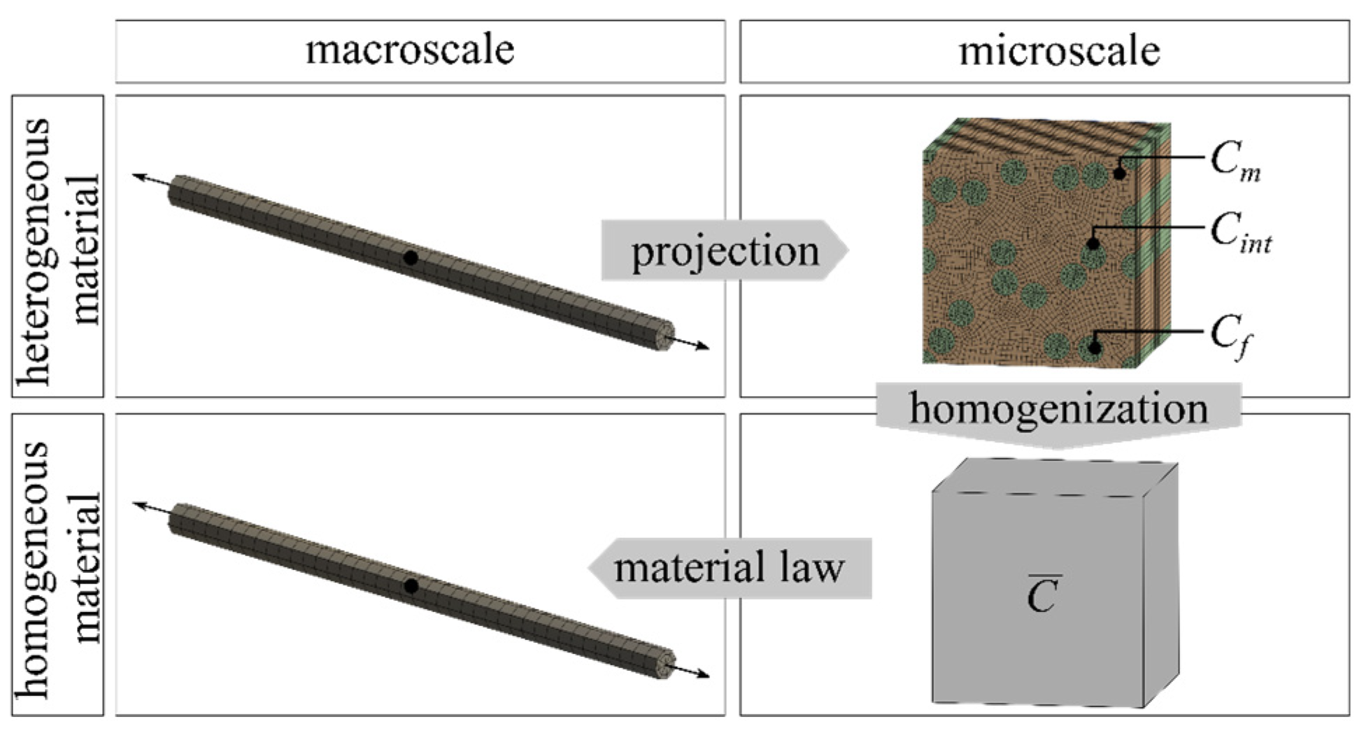
2. FEM
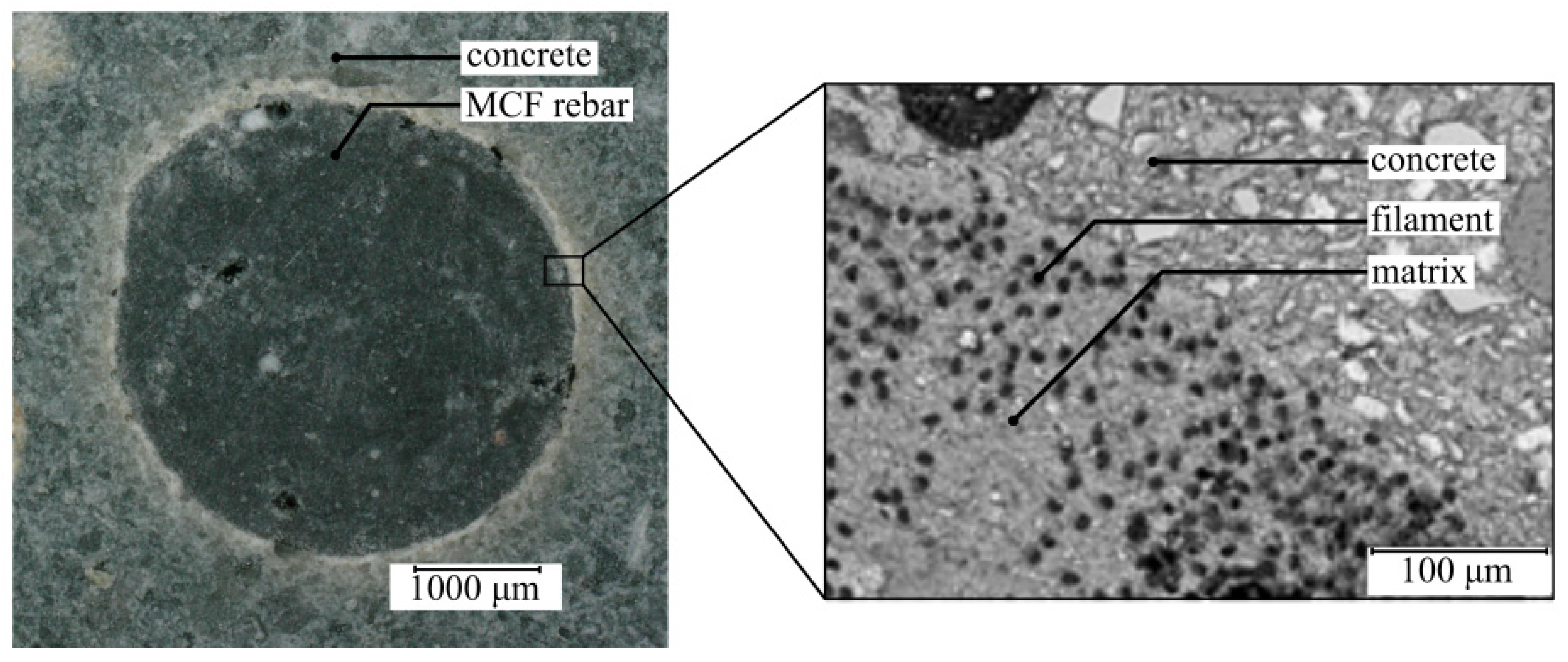
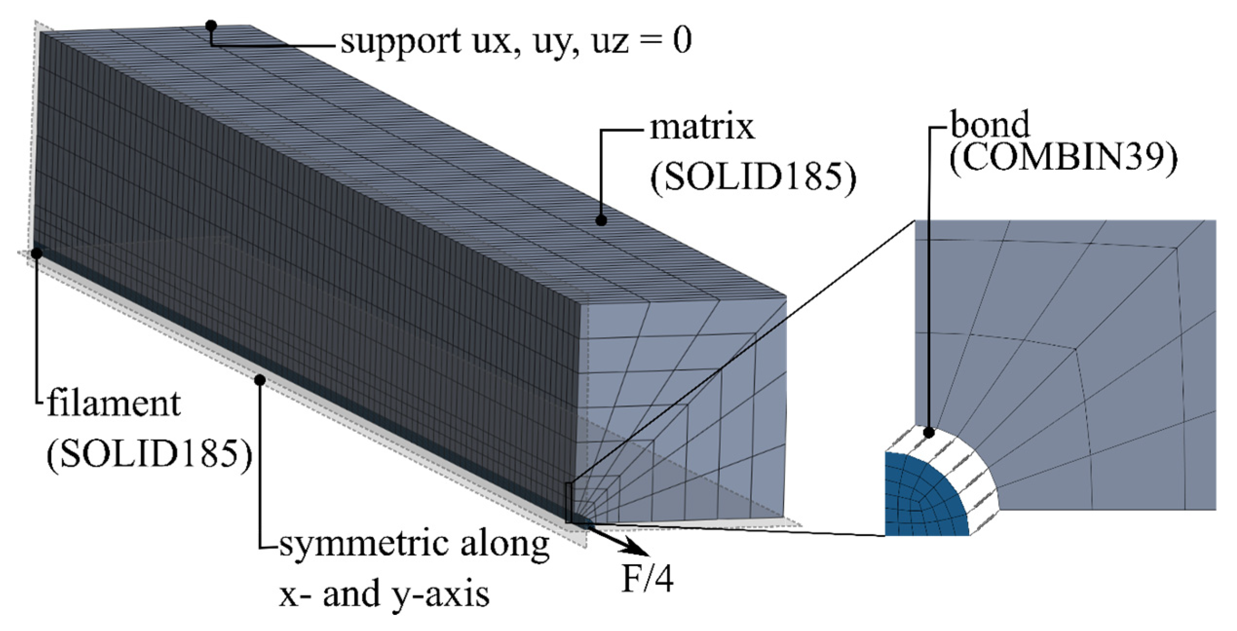
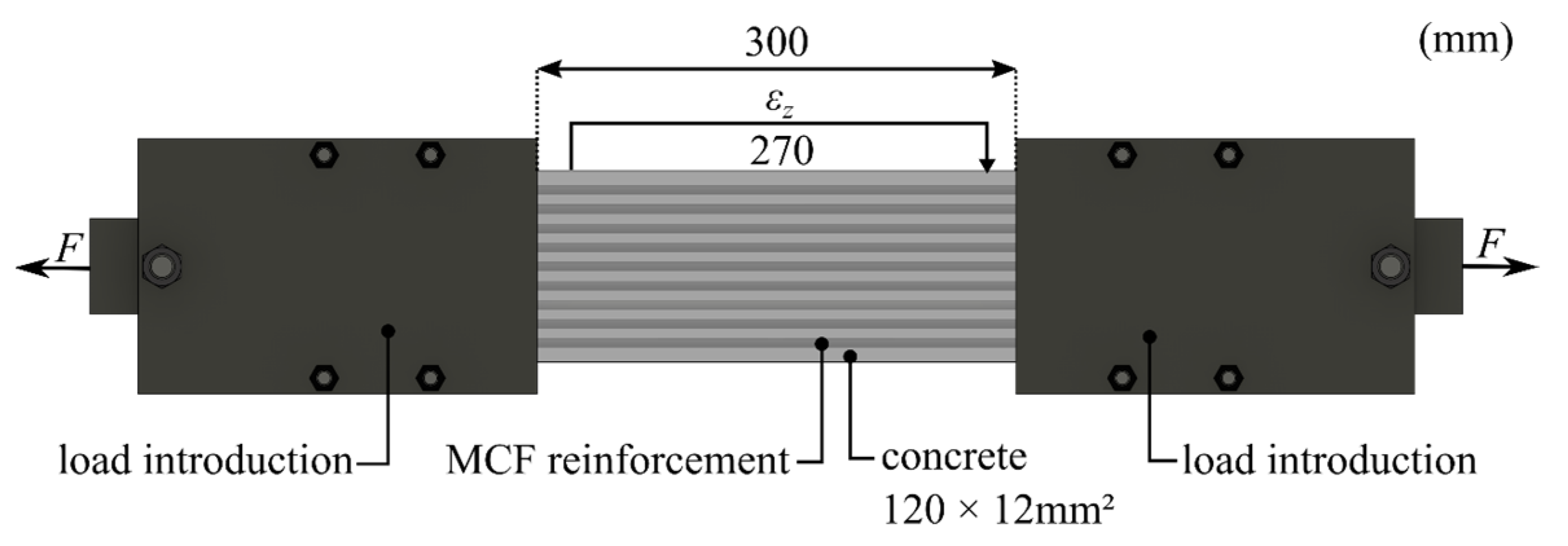
2.1. Model Geometry
- A sufficient quantity of heterogeneities that are randomly distributed. In this case, heterogeneity refers to the filaments embedded in the mineral phase of the MCF-RVE.
- Geometric periodicity.
- The exclusion of discontinuities in the deformation field.
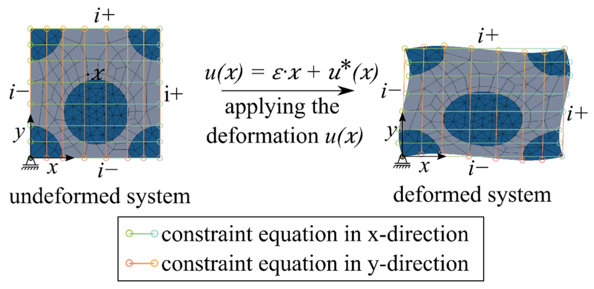
2.2. Boundary Conditions
2.3. Homogenization
3. Material Models of the Individual Phases
3.1. Carbon Filament
3.2. Mineral Matrix
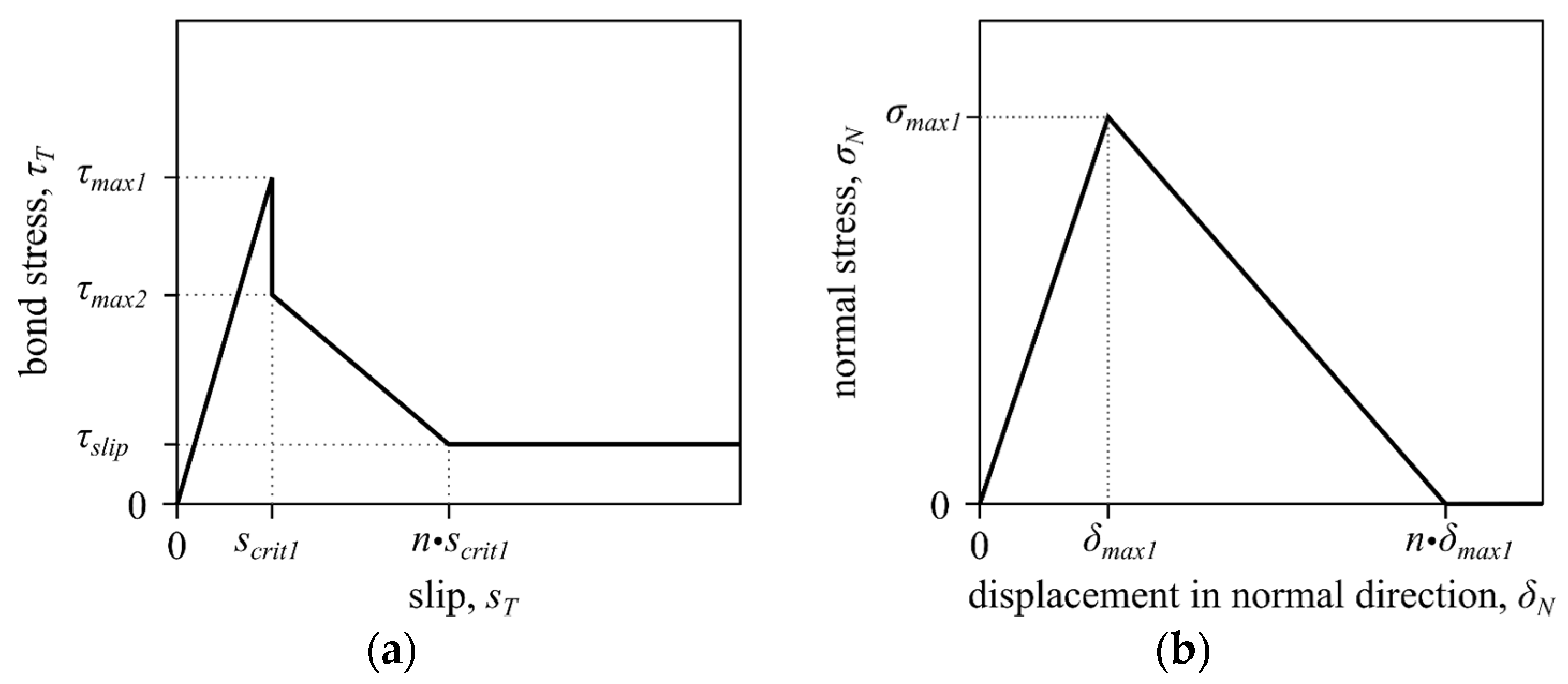
3.3. Bonds between the Filaments and the Matrix
4. Adjustment of the Material Parameters of the Individual Phases
4.1. Filament
4.2. Matrix
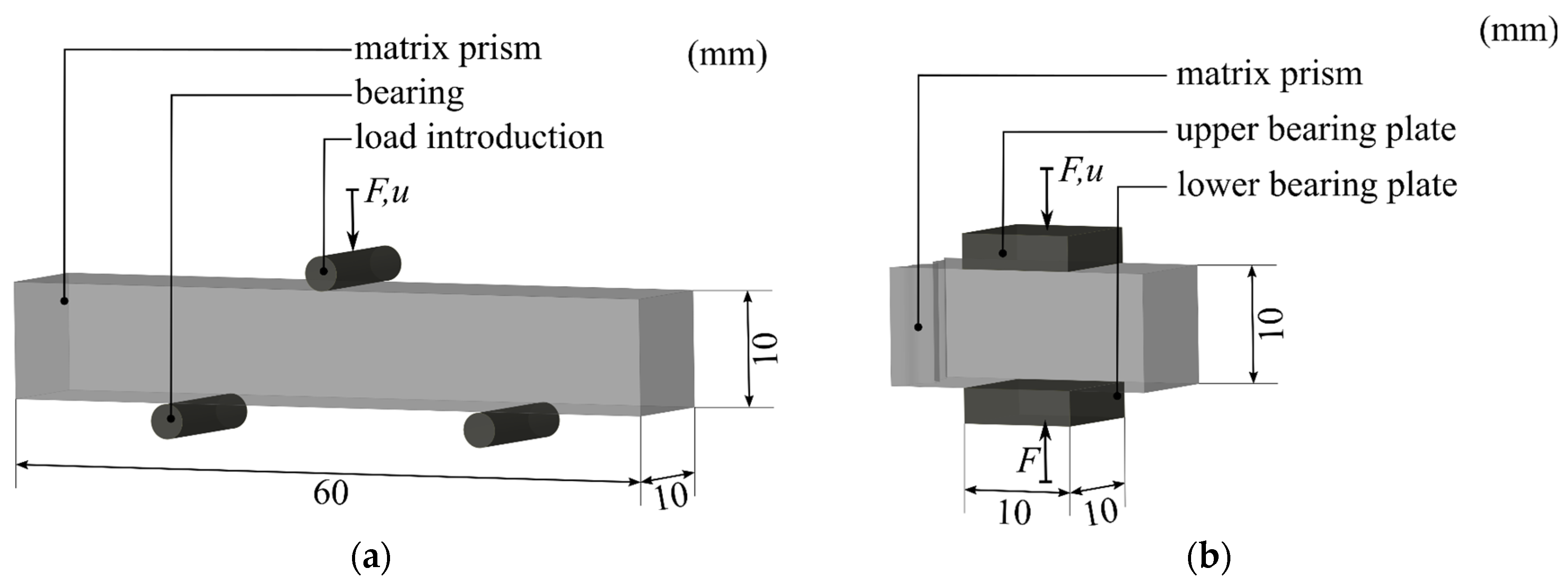
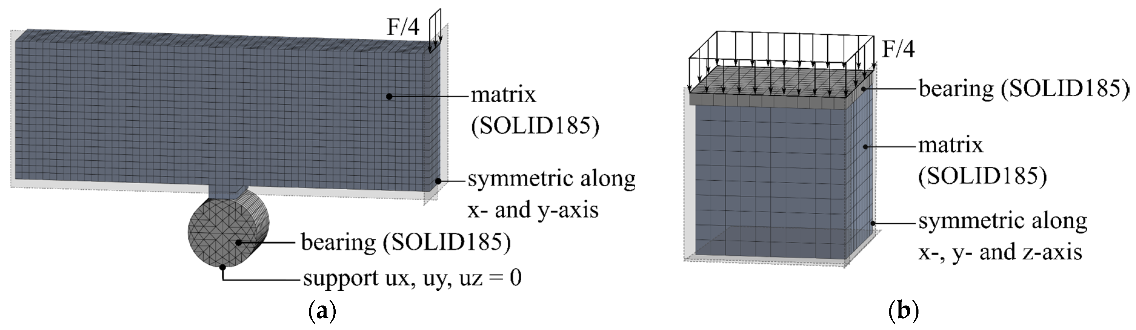
4.2.1. Experimental Studies
4.2.2. Finite Element Model and Results
4.3. Bond between Filament and Matrix
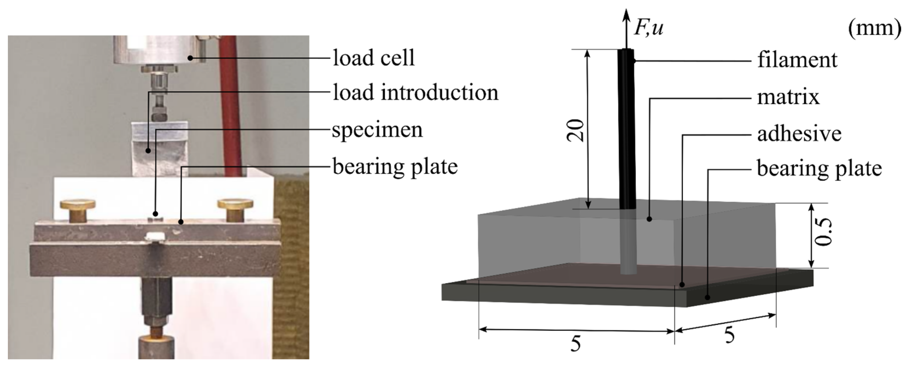
4.3.1. Experimental Studies
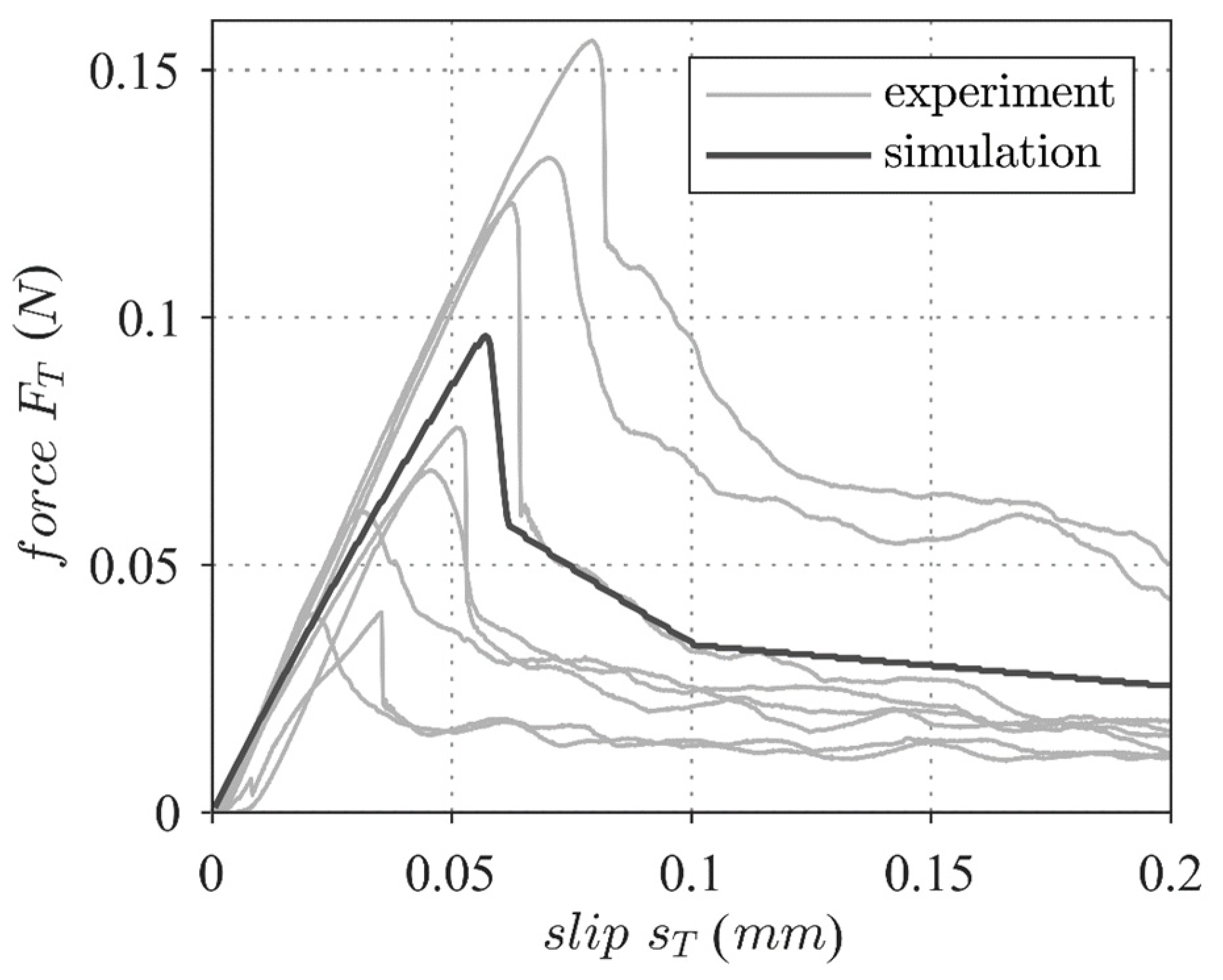
4.3.2. Finite Element Model and Results
5. Validation of the MCF-RVE
6. Sensitivity Analysis
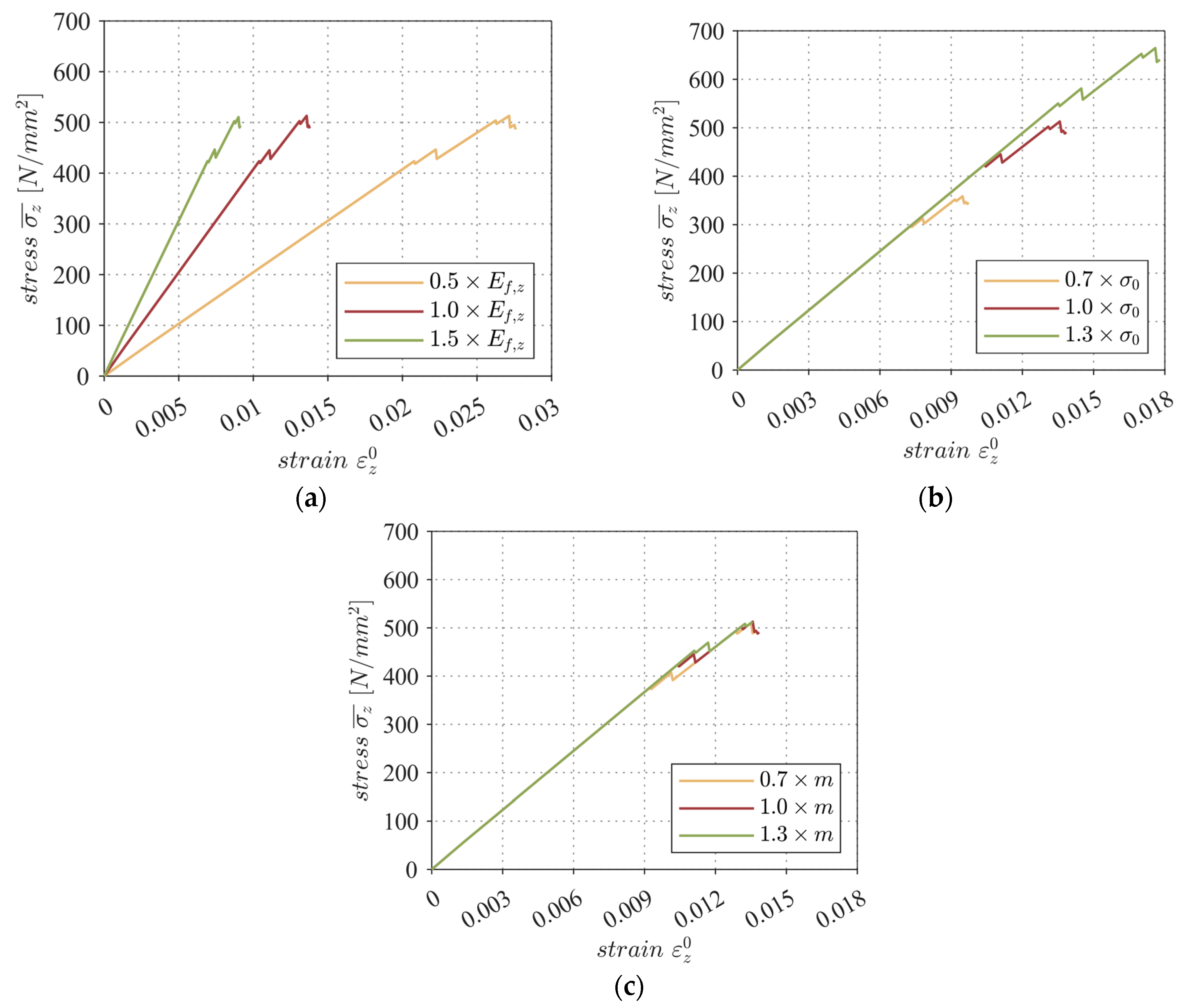
6.1. Sensitivity of Modulus of Elasticity Ef,z
6.2. Sensitivity of Tensile Strength
6.3. Sensitivity of Weibull Module
7. Conclusions
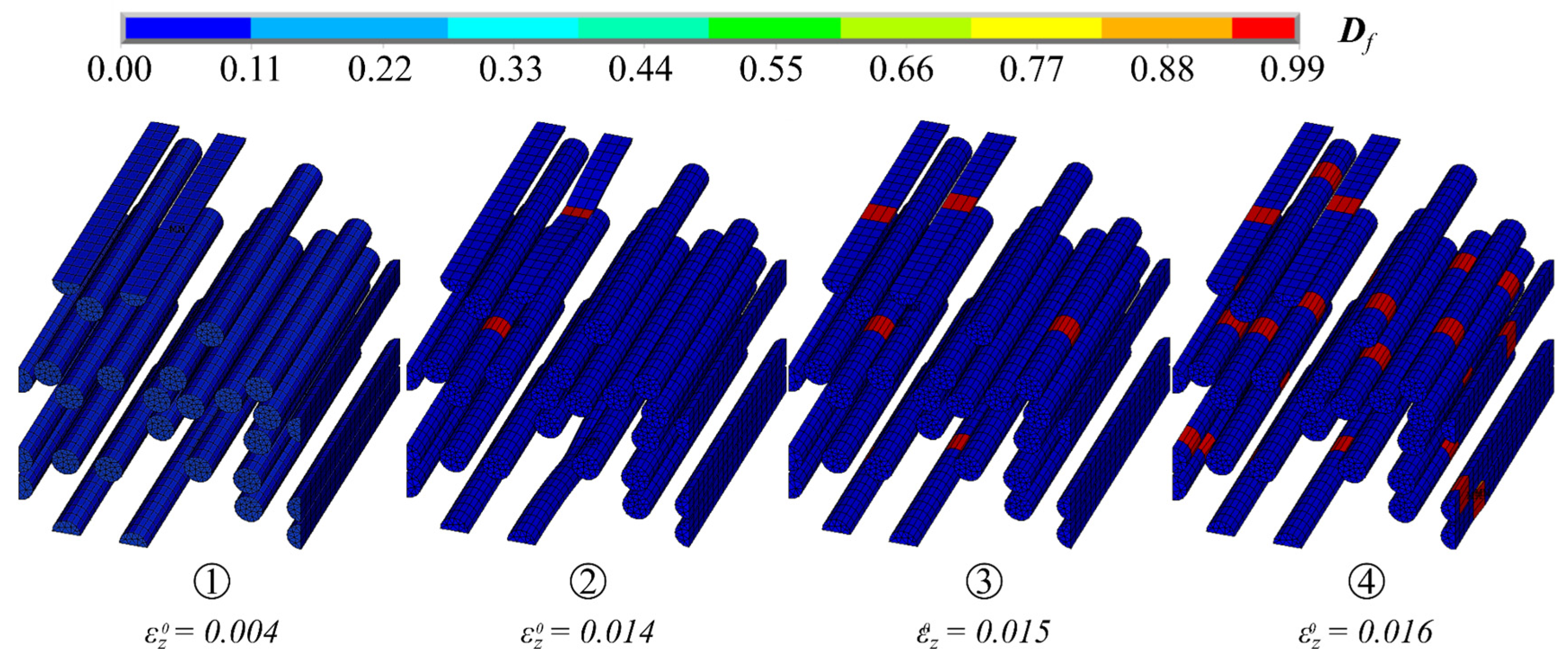
- The MCF-RVE constructed using the adjusted material models enabled the simulation of the degradation behavior as well as the prediction of the effective mechanical behavior of the MCF reinforcement in the longitudinal filament direction. The numerical results were compared with the experimental results. The constructed MCF-RVE was able to capture the dominant mechanical properties of the MCF reinforcement for the considered load type.
- The robustness of the numerical model was evaluated by a sensitivity analysis. The model exhibits high stability and is capable of handling variations in model parameters. The reliability of Wilhelm’s validation set [1] can be attributed to the quality of its data. Nonetheless, it should be noted that the calibration data for certain parameters were obtained from specialized literature rather than being determined through experimental testing.
- The definition of the elastic and damage mechanical parameters of the filaments based on the literature provided adequate results. An experimental determination of the parameters was not necessary, but an adjustment of the average filament strength and the Weibull module could lead to more exact results. The parameters , , and had a decisive influence on the model results.
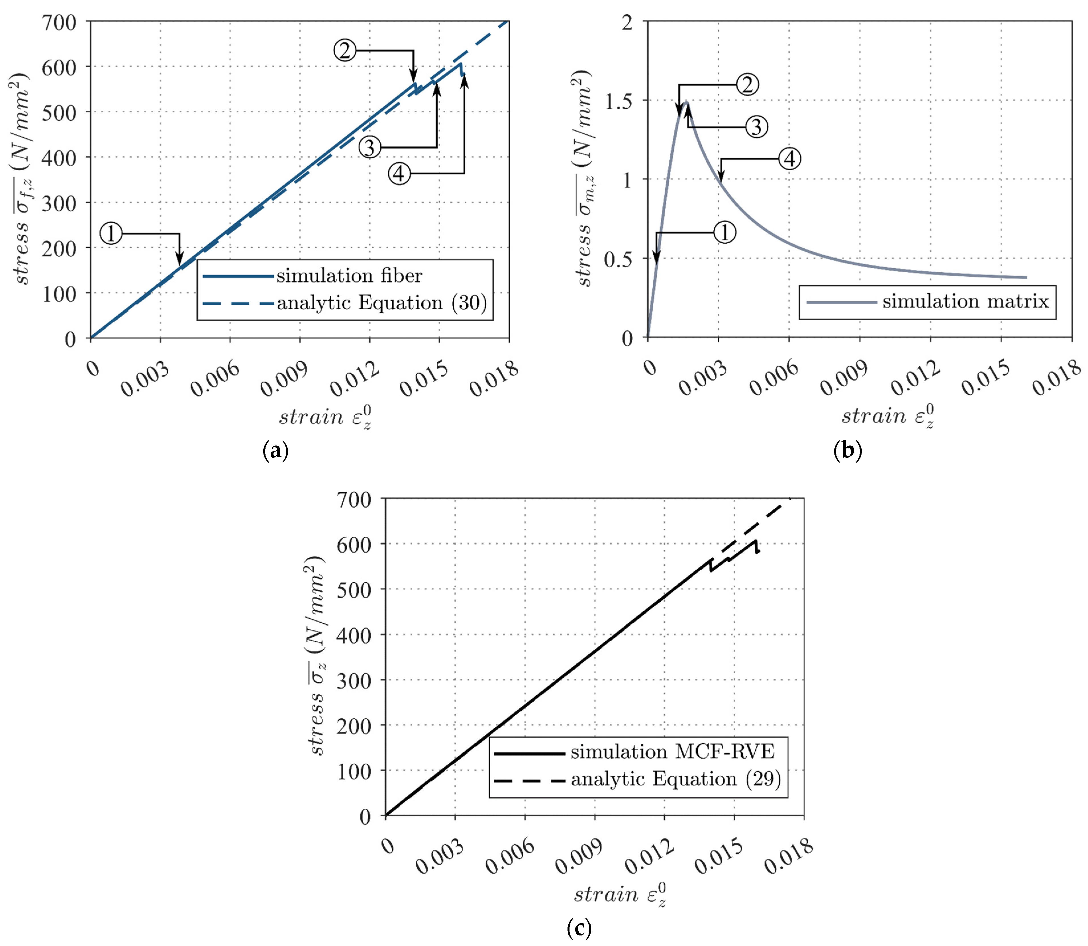
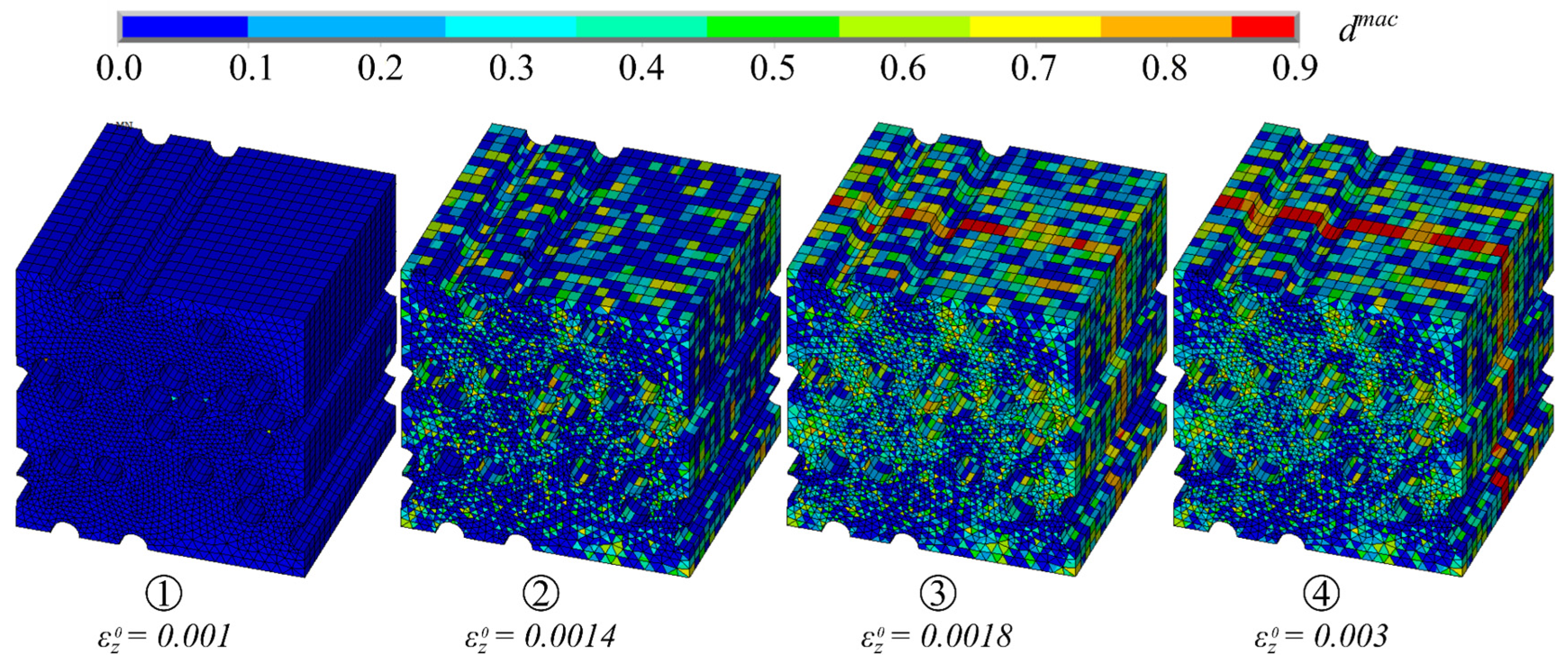
- The validation of the MCF-RVE showed that the influence of the mineral phase on the stiffness and degradation behavior was not significant, as the stiffness of the mineral matrix was significantly smaller than that of the filaments. However, it was necessary to quantify the elastic and tensile mechanical properties of the mineral matrix in advance, as increasing stiffness and strength were accompanied by an increase in the influence of the matrix on the homogenized stress–strain response of the MCF-RVE. In the simulation, the ultimate strength of the MCF reinforcement was approximately 600 N/mm² at a strain of 0.016.
- The analytical bond model of Brameshuber and Banholzer [27] and the spring model of Ngo and Scrodelis [26] enabled the simulation of the bond behavior between the filaments and the mineral matrix. The spring model could be used in the simulation of single-fiber pull-out tests, as well as within the MCF-RVE, for bond simulations. A non-linear simulation of the bond between the reinforcement and the matrix showed no significant influence on the stress–strain response of the MCF-RVE, but a correct formulation of the bond was necessary to quantify the damage mechanisms in the matrix, as well as in the filaments.
Supplementary Materials
Author Contributions
Funding
Institutional Review Board Statement
Informed Consent Statement
Data Availability Statement
Conflicts of Interest
Abbreviations
| Acronyms | |
| ESEM | Environmental scanning electron microscope |
| FE/FEM | Finite element method |
| MCF | Mineral-impregnated carbon fiber |
| RVE | Representative volume element |
| Latin letters | |
| Stiffness tensor | |
| Homogenized stiffness tensor | |
| Damaged stiffness tensor of the filament | |
| Damage tensor of the filament | |
| Variable of damage | |
| Deviatoric part of the second-order unit tensor | |
| Filament diameter | |
| Modulus of elasticity | |
| Force | |
| Force with direction normal to the filament | |
| Force with direction tangential to the filament | |
| Shear modulus | |
| Bulk modulus | |
| Ratio of pressure to tensile strength | |
| Parameters defining the shape of the damage surface | |
| Length of an element | |
| Gauge length | |
| Side length of the representative volume element | |
| Bond length | |
| Weibull module | |
| Factor defining the slip at the transition to the sliding shear stress | |
| Slip | |
| Time step within the simulation | |
| Displacement | |
| Fluctuation within the displacement field | |
| Filament circumference | |
| Volume of the representative volume element | |
| Volumetric part of the second-order unit tensor | |
| 1. Spatial direction orthogonal to the filament | |
| 2. Spatial direction orthogonal to the filament | |
| Spatial direction parallel to the filament | |
| Indexing for filament, matrix, and bond between filament and matrix | |
| Indexing for quantities on the microplane integrated over the solid angle of a unit sphere with a surface area of over the angle | |
| Parameter on the microplane | |
| Greek letters | |
| Maximum degree of degradation | |
| Degradation rate | |
| Damage threshold | |
| History parameter | |
| Distance between opposite node pairs | |
| Relative displacement between a filament and the matrix perpendicular to the filament | |
| Strain | |
| Linear displacement component within a displacement field | |
| Equivalent strain energy | |
| Poisson’s ratio | |
| Stress | |
| Homogenized stress of the representative volume element | |
| Characteristic tensile strength of the filament | |
| Stress of an element within the representative volume element | |
| Maximum normal stress between filament and matrix | |
| Effective normal stress between filament and matrix | |
| Maximum shear stress between filament and matrix | |
| Slip shear stress | |
| Shear stress | |
| Fiber volume fraction | |
| Random number between 0 and 1 | |
| Tensile strength of a filament element | |
| Energy input | |
References
- Wilhelm, K. Bond Behavior of Mineral- and Polymer-Bonded Carbon Reinforcement and Concrete at Room Temperature and Elevated Temperatures up to 500 °C. Ph.D. Thesis, Technische Universität Dresden, Dresden, Germany, 2021. [Google Scholar]
- Mechtcherine, V.; Michel, A.; Liebscher, M.; Schneider, K.; Großmann, C. Mineral-impregnated carbon fiber composites as novel reinforcement for concrete construction: Material and automation perspectives. Autom. Constr. 2020, 110, 103002. [Google Scholar] [CrossRef]
- Schneider, K.; Michel, A.; Liebscher, M.; Terreri, L.; Hempel, S.; Mechtcherine, V. Mineral-impregnated carbon fibre reinforcement for high temperature resistance of thin-walled concrete structures. Cem. Concr. Compos. 2019, 97, 68–77. [Google Scholar] [CrossRef]
- Nguyen, V.P.; Stroeven, M. Multiscale continuous and discontinuous modeling of heterogeneous materials: A review on recent developments. J. Multiscale Model. 2011, 3, 229–270. [Google Scholar] [CrossRef]
- Hill, R. A self-consistent mechanics of composite materials. J. Mech. Phys. Solids 1965, 13, 213–222. [Google Scholar] [CrossRef]
- Zastrau, B.; Lepenies, I.; Richter, M. On the Multi Scale Modeling of Textile Reinforced Concrete. Tech. Mech.-Eur. J. Eng. Mech. 2008, 28, 53–63. [Google Scholar]
- Feyel, F. A multilevel finite element method (FE2) to describe the response of highly non-linear structures using generalized continua. Comput. Methods Appl. Mech. Eng. 2003, 192, 3233–3244. [Google Scholar] [CrossRef]
- Fuchs, A.; Curosu, I.; Kaliske, M. Numerical Mesoscale Analysis of Textile Reinforced Concrete. Materials 2020, 13, 3944. [Google Scholar] [CrossRef] [PubMed]
- Shaik, A.; Salvi, A. A Multi Scale Approach for Analysis of Fiber Reinforced Composites. Mater. Today Proc. 2017, 4, 3197–3206. [Google Scholar] [CrossRef]
- Gallyamov, E.R.; Cuba Ramos, A.I.; Corrado, M.; Rezakhani, R.; Molinari, J.-F. Multi-scale modelling of concrete structures affected by alkali-silica reaction: Coupling the mesoscopic damage evolution and the macroscopic concrete deterioration. Int. J. Solids Struct. 2020, 207, 262–278. [Google Scholar] [CrossRef]
- Böhm, H.J. A Short Introduction to Basic Aspects of Continuum Micromechanics; Publication No. CDL-FMD Report 3-1998; Institute of Lightweight Design and Structural Biomechanics: Vienna, Austria, 2018. [Google Scholar]
- Tavares, R.P.; Melro, A.R.; Bessa, M.A.; Turon, A.; Liu, W.K.; Camanho, P.P. Mechanics of hybrid polymer composites: Analytical and computational study. Comput. Mech. 2016, 3, 405–421. [Google Scholar] [CrossRef]
- Feder, J. Random sequential adsorption. J. Theor. Biol. 1980, 2, 237–254. [Google Scholar] [CrossRef]
- Buryachenko, V.A.; Pagano, N.J.; Kim, R.Y.; Spowart, J.E. Quantitative description and numerical simulation of random microstructures of composites and their effective elastic moduli. Int. J. Solids Struct. 2003, 1, 47–72. [Google Scholar] [CrossRef]
- Melro, A.R. Analytical and Numerical Modelling of Damage and Fracture of Advanced Composites. Ph.D. Thesis, University of Porto, Porto, Portugal, 2011. [Google Scholar]
- Haddani, F.; Maliki, A.E.; Lkouen, A. Random Microstructure Generation. In Proceedings of the 2nd International Conference on Embedded Systems and Artificial Intelligence (ESAI’21), Fez, Morocco, 1–2 April 2021. [Google Scholar]
- Hayder, H.M.S.; Afrasiab, H.; Gholami, M. Efficient generation of random fiber distribution by combining random sequential expansion and particle swarm optimization algorithms. Compos. Part A 2023, 173, 107649. [Google Scholar] [CrossRef]
- Smit, R.J.M.; Brekelmans, W.A.M.; Meijer, H.E.H. Prediction of the mechanical behavior of nonlinear heterogeneous systems by multi-level finite element modeling. Comput. Methods Appl. Mech. Eng. 1998, 155, 181–192. [Google Scholar] [CrossRef]
- Huang, H.; Talreja, R. Effects of void geometry on elastic properties of unidirectional fiber reinforced composites. Compos. Sci. Technol. 2005, 13, 1964–1981. [Google Scholar] [CrossRef]
- Xia, Z.; Zhang, Y.; Ellyin, F. A unified periodical boundary conditions for representative volume elements of composites and applications. Int. J. Solids Struct. 2003, 8, 1907–1921. [Google Scholar] [CrossRef]
- Soden, P. Lamina properties, lay-up configurations and loading conditions for a range of fibre-reinforced composite laminates. Compos. Sci. Technol. 1998, 7, 1011–1022. [Google Scholar] [CrossRef]
- Barbero, E.J. Finite Element Analysis of Composite Materials; CRC Press: Boca Raton, FL, USA, 2008; pp. 203–206. [Google Scholar]
- Weibull, W. A Statistical Distribution Function of Wide Applicability. J. Appl. Sci. 1951, 3, 293–297. [Google Scholar] [CrossRef]
- ANSYS Inc. ANSYS Advanced Analysis Techniques Guide; ANSYS Inc.: Canonsburg, PA, USA, 2005. [Google Scholar]
- Leukart, M.; Ramm, E. A comparison of damage models formulated on different material scales. Comput. Mater. Sci. 2003, 28, 749–762. [Google Scholar] [CrossRef]
- Ngo, D.; Scrodelis, A.C. Finite Element Analysis of Reinforced Concrete Beams. ACI J. Proc. 1967, 64, 152–163. [Google Scholar]
- Brameshuber, W.; Banholzer, B. Eine Methode zur Beschreibung des Verbundes zwischen Faser und zementgebundener Matrix. Beton- Und Stahlbetonbau 2001, 96, 663–669. [Google Scholar]
- Cosenza, E.; Manfredi, G.; Realfonzo, R. Behavior and Modeling of Bond of FRP Rebars to Concrete. J. Compos. Constr. 1997, 1, 40–51. [Google Scholar] [CrossRef]
- FIB. Fib Model Code for Concrete Structures 2010; International Federation for Structural Concrete: Lausanne, Switzerland, 2013. [Google Scholar]
- Focacci, F.; Nanni, A.; Bakis, C.E. Local Bond-Slip Relationship for FRP Reinforcement in Concrete. J. Compos. Constr. 2000, 4, 24–31. [Google Scholar] [CrossRef]
- Eligehausen, R.; Popov, E.P.; Bertero, V.V. Local Bond Stress-Slip Relationships of deformed bars under generalized excitations. In Experimental Results and Analytical Model; National Science Foundation: Berkeley, CA, USA, 1983. [Google Scholar]
- Häussler-Combe, U.; Shehni, A.; Chihadeh, A. Finite element modeling of fiber reinforced cement composites using strong discontinuity approach with explicit representation of fibers. Int. J. Solids Struct. 2020, 200, 213–230. [Google Scholar] [CrossRef]
- Zhandanarov, S.; Mäder, S. Characterization of fiber/matrix interface strength: Applicability of different tests, approaches and parameters. Compos. Sci. Technol. 2005, 65, 149–160. [Google Scholar] [CrossRef]
- Henriques, J.; Simões da Silva, L.; Valente, I.B. Numerical modeling of composite beam to reinforced concrete wall joints. Eng. Struct. 2013, 52, 747–761. [Google Scholar] [CrossRef]
- Hoppe, L. Numerical simulation of fiber-matrix debonding in single fiber pull-out tests. GAMM Arch. Stud. 2020, 2, 21–35. [Google Scholar] [CrossRef]
- Pathak, P.; Zhang, Y.X. Numerical study of structural behavior of fiber-reinforced polymer-strengthened reinforced concrete beams with bond-slip effect under cyclic loading. Struct. Concr. 2019, 20, 97–107. [Google Scholar] [CrossRef]
- Keuser, M.; Mehlhorn, G.; Cornelius, V. Bond Between Prestressed Steel and Concrete—Computer Analysis using ADINA. Comput. Struct. 1983, 17, 669–676. [Google Scholar]
- Curtin, W.A.; Takeda, N. Tensile Strength of Fiber-Reinforced Composites: II. Application to Polymer Matrix Composites. J. Compos. Mater. 1998, 3, 2060–2081. [Google Scholar] [CrossRef]
- Karpiesiuk, J.; Chyzy, T. Young’s modulus and Poisson’s ratio of the deformable cement adhesives. Sci. Eng. Compos. Mater. 2020, 27, 299–307. [Google Scholar] [CrossRef]
- DIN EN 12390-3; Prüfung von Festbeton—Teil 3: Druckfestigkeit von Probekörpern; Deutsche Fassung EN 12390-3:2019. Beuth Verlag GmbH: Berlin, Germany, 2019.
- DIN EN 12390-5; Prüfung von Festbeton—Teil 5: Biegezugfestigkeit von Probekörpern; Deutsche Fassung EN 12390-5:2019. Beuth Verlag GmbH: Berlin, Germany, 2019.
- DIN EN 196-1; Prüfverfahren für Zement—Teil 1: Bestimmung der Festigkeit. Beuth Verlag GmbH: Berlin, Germany, 2016.
- Rabbat, B.G.; Russell, H.G. Friction Coefficient of Steel on Concrete or Grout. J. Struct. Eng. 1985, 111, 505–515. [Google Scholar] [CrossRef]
- Mattei, L.; Di Puccio, F. Frictionless vs. Frictional Contact in Numerical Wear Predictions of Conformal and Non-conformal Sliding Couplings. Tribol. Lett. 2022, 70, 115. [Google Scholar] [CrossRef]
- Ranjbarian, M.; Mechtcherine, V. A novel test setup for the characterization of bridging behaviour of single microfibres embedded in a mineral-based matrix. Cem. Concr. Compos. 2018, 92, 92–101. [Google Scholar] [CrossRef]
- Constâncio Trindade, A.C.; Curosu, I.; Liebscher, M.; Mechtcherine, V.; de Andrade Silva, F. On the mechanical performance of K- and Na-based strain-hardening geopolymer composites (SHGC) reinforced with PVA fibers. Constr. Build. Mater. 2020, 248, 118558. [Google Scholar] [CrossRef]
- Zanuy, C.; Curbach, M.; Lindorf, A. Finite element study of bond strength between concrete and reinforcement under uneven confinement condition. Struct. Concr. 2013, 14, 260–270. [Google Scholar] [CrossRef]
- Zobel, R.; Curbach, M. Bond modelling of reinforcing steel under transverse tension. In Proceedings of the Fib Symposium–Concrete–Innovation and Design; Tivoli Congress Center: Copenhagen, Denmark, 2015. [Google Scholar]
- Zobel, R.; Curbach, M. Numerical study of reinforced and prestressed concrete components under biaxial tensile stresses. Struct. Concr. 2017, 18, 356–365. [Google Scholar] [CrossRef]
- Mallick, P.K. Fiber-reinforced composites. In Materials, Manufacturing and Design; Mechanical Engineering No. 83; Dekker: New York, NY, USA, 1993. [Google Scholar]


| 1. | Read the strain of the element at time t |
| 2. | Calculate the stress at time t |
| 3. | Update the history variable |
| 4. | Calculate the degradation |
| 5. | Determine the stress and the stiffness tensor at time t |
| Material Property | Value | Source |
|---|---|---|
| (mm) | 0.0069 | [1] |
| Modulus of elasticity | ||
| (N/mm²) | 15,000 | [21] |
| (N/mm²) | 230,000 | [21] |
| 0.2 | [21] | |
| Shear modulus | ||
| (N/mm²) | 15,000 | [21] |
| (N/mm²) | 7000 | [21] |
| Weibull parameters | ||
| (N/mm²) | 3170 | [38] |
| 5.1 | [38] | |
| (mm) | 25 | [38] |
| Elasticity Variables | Damage Model | ||||
|---|---|---|---|---|---|
| (N/mm²) | |||||
| 1350 | 0.15 | 180 | 0.95 | 40 | 0.00065 (0.000163) |
| (N/mm²) | (N/mm²) | (N/mm²) | (mm) | |
|---|---|---|---|---|
| 7.85 | 4.71 | 3.00 | 0.055 | 1.82 |
Disclaimer/Publisher’s Note: The statements, opinions and data contained in all publications are solely those of the individual author(s) and contributor(s) and not of MDPI and/or the editor(s). MDPI and/or the editor(s) disclaim responsibility for any injury to people or property resulting from any ideas, methods, instructions or products referred to in the content. |
© 2024 by the authors. Licensee MDPI, Basel, Switzerland. This article is an open access article distributed under the terms and conditions of the Creative Commons Attribution (CC BY) license (https://creativecommons.org/licenses/by/4.0/).
Share and Cite
Zernsdorf, K.; Mechtcherine, V.; Curbach, M.; Bösche, T. Numerical Material Testing of Mineral-Impregnated Carbon Fiber Reinforcement for Concrete. Materials 2024, 17, 737. https://doi.org/10.3390/ma17030737
Zernsdorf K, Mechtcherine V, Curbach M, Bösche T. Numerical Material Testing of Mineral-Impregnated Carbon Fiber Reinforcement for Concrete. Materials. 2024; 17(3):737. https://doi.org/10.3390/ma17030737
Chicago/Turabian StyleZernsdorf, Kai, Viktor Mechtcherine, Manfred Curbach, and Thomas Bösche. 2024. "Numerical Material Testing of Mineral-Impregnated Carbon Fiber Reinforcement for Concrete" Materials 17, no. 3: 737. https://doi.org/10.3390/ma17030737
APA StyleZernsdorf, K., Mechtcherine, V., Curbach, M., & Bösche, T. (2024). Numerical Material Testing of Mineral-Impregnated Carbon Fiber Reinforcement for Concrete. Materials, 17(3), 737. https://doi.org/10.3390/ma17030737