Fabric Weave Pattern and Yarn Color Recognition and Classification Using a Deep ELM Network

Abstract
:1. Introduction
2. Method
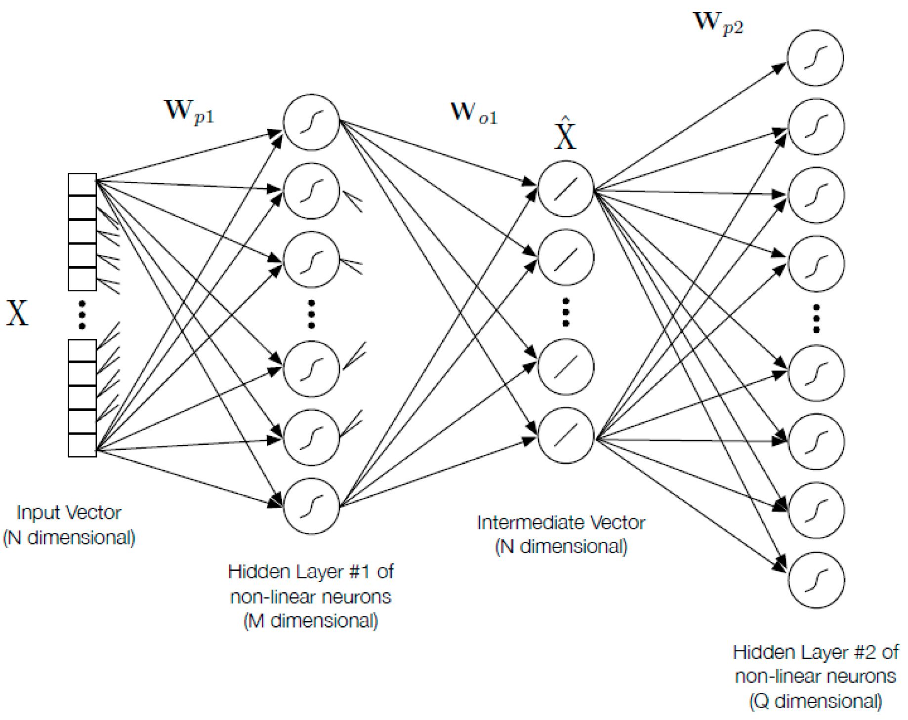
2.1. Biologically-Inspired Deep ELM-Based Pattern Recognition Network Design (D-ELM)
2.2. Parameter Selection of the Deep ELM Network
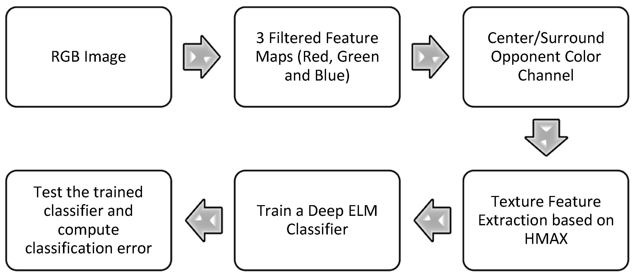
2.3. Brief Description of Color HMAX Based Feature Descriptor (Opponent Color Channels)
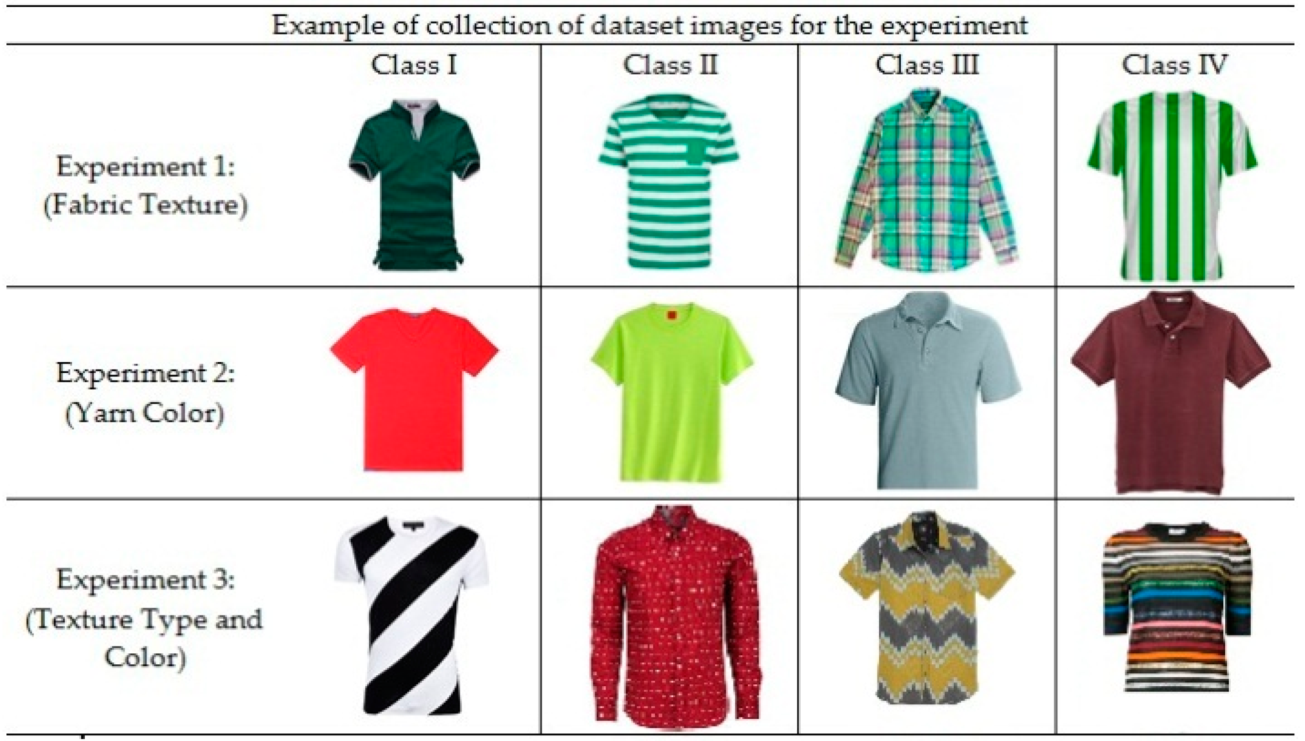
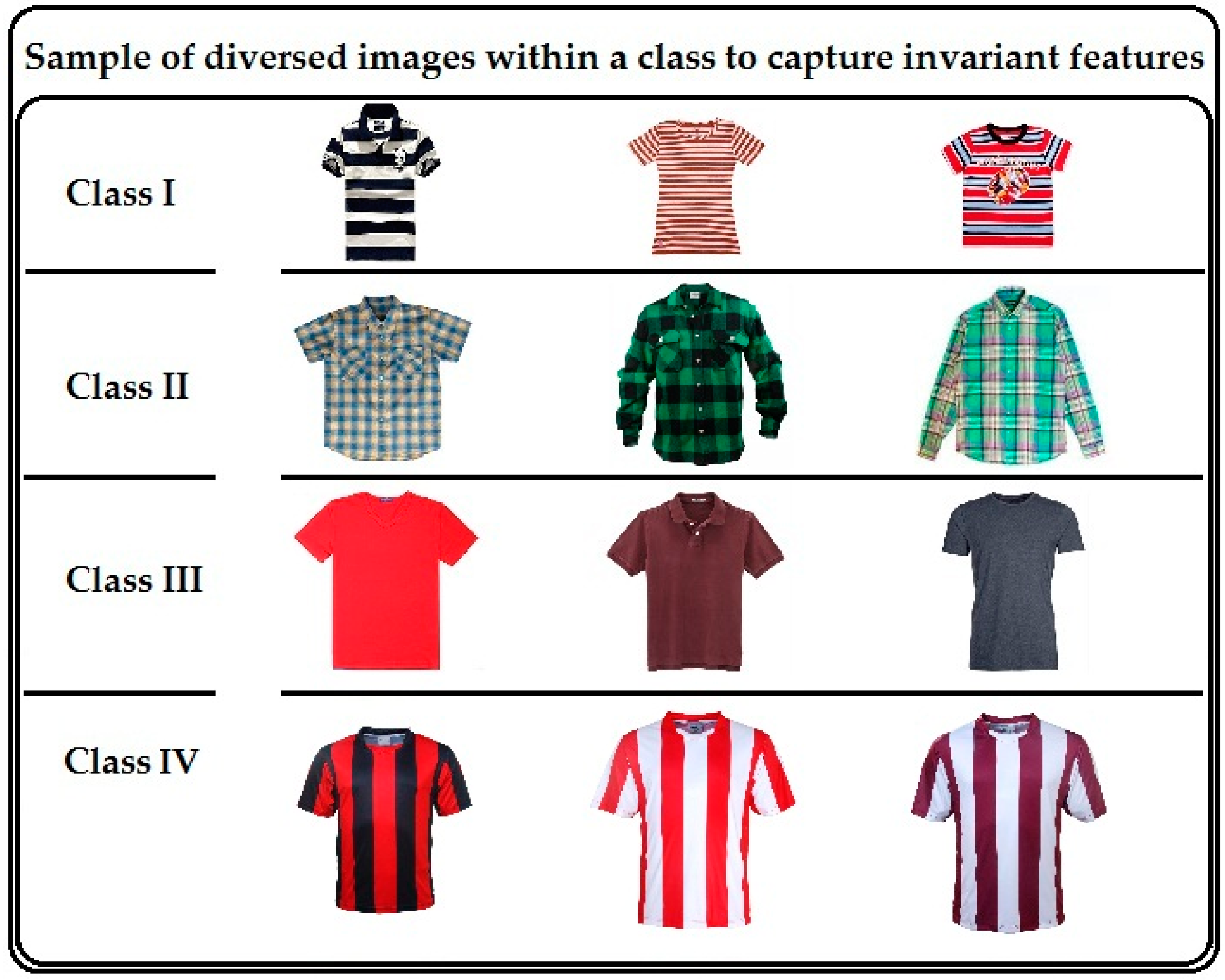
3. Experiments
4. Results and Discussion
5. Conclusions
Acknowledgments
Author Contributions
Conflicts of Interest
References
- Haralick, R.M.; Shaunmmugam, K.; Dinstein, I. Textural Features for Image Classification. IEEE Trans. Syst. Man Cybern. 1973, 3, 610–620. [Google Scholar] [CrossRef]
- Xu, B. Identifying Fabric Structures with Fast Fourier Transform Techniques. Text. Res. J. 1996, 66, 496–506. [Google Scholar]
- Ravandi, S.A.H.; Toriumi, K. Fourier Transform Analysis of Plain Weave Fabric Appearance. Text. Res. J. 1995, 65, 676–683. [Google Scholar] [CrossRef]
- Huang, C.C.; Liu, S.C.; Yu, W.H. Woven Fabric Analysis by Image Processing Part I: Identification of Weave Patterns. Text. Res. J. 2000, 70, 481–485. [Google Scholar] [CrossRef]
- Kang, T.J.; Choi, S.H.; Kin, S.M. Automatic Recognition of Fabric Weave Patterns by Digital Image Analysis. Text. Res. J. 1999, 69, 77–83. [Google Scholar] [CrossRef]
- Kuo, C.F.J.; Shih, C.Y.; Kao, C.Y.; Lee, J.Y. Automatic Recognition of Fabric Weave Patterns by Fuzzy C-Means Clustering Method. Text. Res. J. 2004, 74, 107–111. [Google Scholar] [CrossRef]
- Wang, L.; He, D.C. A New Statistical Approach for Texture Analysis. Photogramm. Eng. Remote Sens. 1990, 56, 61–66. [Google Scholar]
- Xin, B.; Hu, J.; Baciu, G.; Yu, X. Investigation on the Classification of Weave Pattern based on an Active Grid Model. Text. Res. J. 2009, 79, 1123–1134. [Google Scholar]
- Guo, Z.; Zhang, D.; Zhang, L.; Zuo, W. Palmprint Verification Using Binary Orientation Co-Occurrence Vector. Pattern Recognit. Lett. 2009, 30, 1219–1227. [Google Scholar] [CrossRef]
- Potiyaraj, P.; Subhakalin, C.; Sawangharsub, B.; Udomkichdecha, W. Recognition and Revisualization of Woven Fabric Structures. Int. J. Cloth. Sci. Tech. 2010, 22, 79–87. [Google Scholar] [CrossRef]
- Alvarenga, A.V.; Teixeira, C.A.; Ruano, M.G.; Pereira, W.C.A. Influence of Temperature Variations on the Entropy and Correlation of the Grey-Level Co-Occurrence Matrix from B-Mode Images. Ultrasonics 2010, 50, 290–293. [Google Scholar] [CrossRef] [PubMed]
- Hu, Y.; Zhao, C.X.; Wang, H.N. Directional Analysis of Texture Images Using Gray Level Co-Occurrence Matrix. In Proceedings of the IEEE Pacific-Asia Workshop on Computational Intelligence and Industrial Application, Wuhan, China, 19–20 December 2008. [Google Scholar]
- Zhang, J.; Xie, Z.; Gao, J.; Wu, K. Beyond Shape: Incorporating Color Invariance into a Biologically Inspired Feed-Forward Model of Category Recognition. In Proceedings of the 7th Indian Conference on Computer Vision, Graphics and Image Processing, Chennai, India, 12–15 December 2010; pp. 85–92. [Google Scholar]
- Jalali, S.; Tan, C.; Lim, J.; Tham, J.; Ong, S.; Seekings, P.; Taylor, E. Visual Recognition Using a Combination of Shape and Color Features. In Proceedings of the Annual Conference of the Cognitive Science Society, Berlin, Germany, 29 July–3 August 2013; pp. 2638–2643. [Google Scholar]
- Zhao, H.; Zhou, B.; Liu, P.; Zhao, T. Modulating a Local Shape Descriptor through Biologically Inspired Color Feature. J. Bionic Eng. 2014, 2, 311–321. [Google Scholar] [CrossRef]
- Conway, B.R.; Chatterjee, S.; Field, G.D.; Horwitz, G.D.; Johnson, E.N.; Koida, K.; Mancuso, K. Advances in color science: From retina to behavior. J. Neurosci. 2010, 30, 14955–14963. [Google Scholar] [CrossRef] [PubMed]
- Khan, B.; Han, F.; Wang, Z.J.; Masood, R. Bio-Inspired Approach to Invariant Recognition and Classification of Fabric Weave Patterns and Yarn Color. Assem. Autom. 2016, 36, 152–158. [Google Scholar] [CrossRef]
- Furber, S.B.; Galluppi, F.; Temple, S.; Plana, L.A. The SpiNNaker Project. Proc. IEEE 2014, 102, 652–665. [Google Scholar] [CrossRef]
- Benjamin, B.V.; Gao, P.; McQuinn, E.; Choudhary, S.; Chandrasekaran, A.R.; Bussat, J.M.; Alvarez-Icaza, R.; Arthur, J.V.; Merolla, P.A.; Boahen, K. Neurogrid: A mixed Analog–Digital Multichip System for Large-Scale Neural Simulations. Proc. IEEE 2014, 102, 699–716. [Google Scholar] [CrossRef]
- Tissera, M.D.; McDonnell, M.D. Deep extreme learning machines: Supervised autoencoding architecture for classification. J. Neurocomput. 2016, 174, 42–49. [Google Scholar] [CrossRef]
- Eliasmith, C.; Anderson, C.H. Neural Engineering: Computation, Representation, and Dynamics in Neurobiological Systems; The MIT Press: Cambridge, MA, USA, 2003. [Google Scholar]
- Huang, G.B.; Zhu, Q.Y.; Siew, C.K. Extreme learning machine: Theory and applications. Neurocomputing 2006, 70, 489–501. [Google Scholar] [CrossRef]
- Huang, G.B.; Wang, D.H.; Lan, Y. Extreme learning machines: A survey. Int. J. Mach. Learn. Cybern. 2011, 2, 107–122. [Google Scholar] [CrossRef]
- Cambria, E.; Huang, G.B. Extreme learning machines. IEEE Intell. Syst. 2013, 28, 30–31. [Google Scholar] [CrossRef]
- Penrose, R. A generalized inverse for matrices. Math. Proc. Camb. Philos. Soc. 1955, 51, 406–413. [Google Scholar] [CrossRef]
- Huang, G.B. An insight into extreme learning machines: random neurons, random features and kernels. Cognit. Comput. 2014, 6, 376–390. [Google Scholar] [CrossRef]
- Kasun, L.L.C.; Zhou, H.; Huang, G.B. Representational learning with ELMs for big data. IEEE Intell. Syst. 2013, 28, 31–34. [Google Scholar]
- Yu, W.; Zhuang, F.; He, Q.; Shi, Z. Learning deep representations via extreme learning machines. Neurocomputing 2015, 149, 308–315. [Google Scholar] [CrossRef]
- Han, H.G.; Wang, L.D.; Qiao, J.F. Hierarchical extreme learning machine for feedforward neural network. Neurocomputing 2014, 128, 128–135. [Google Scholar]
- Basu, A.; Shuo, S.; Zhou, H.; Lim, M.H.; Huang, G.B. Silicon spiking neurons for hardware implementation of extreme learning machines. Neurocomputing 2013, 102, 125–134. [Google Scholar] [CrossRef]
- Galluppi, F.; Davies, S.; Furber, S.; Stewart, T.; Eliasmith, C. Real time on-chip implementation of dynamical systems with spiking neurons. In Proceedings of the International Joint Conference on Neural Networks IJCNN, Brisbane, Australia, 10–15 June 2012; pp. 1–8. [Google Scholar]
- Choudhary, S.; Sloan, S.; Fok, S.; Neckar, A.; Trautmann, E.; Gao, P.; Stewart, T.; Eliasmith, C.; Boahen, K. Silicon neurons that compute. In Proceedings of the International Conference on Artificial Neural Networks and Machine Learning (ICANN 2012), Lausanne, Switzerland, 11–14 September 2012; pp. 121–128. [Google Scholar]
- Tapson, J.; van Schaik, A. Learning the pseudo inverse solution to network weights. Neural Netw. 2013, 45, 94–100. [Google Scholar] [CrossRef] [PubMed]
- Bengio, Y. Learning deep architectures for AI. Found. Trends Mach. Learn. 2009, 2, 1–127. [Google Scholar] [CrossRef]
- Hinton, G.E.; Osindero, S.; Teh, Y.W. A fast learning algorithm for deep belief nets. Neural Comput. 2006, 18, 1527–1554. [Google Scholar] [CrossRef] [PubMed]
- Schmidhuber, J. Deep learning in neural networks: An overview. Neural Netw. 2015, 61, 85–117. [Google Scholar] [CrossRef] [PubMed]
- McDonnell, M.D.; Tissera, M.D.; Ladusich, T.V.; van Schaik, A.; Tapson, J. Fast, simple and accurate handwritten digit classification by training shallow neural network classifiers with the extreme learning machine algorithm. PLOS ONE 2015, 10, e0134254. [Google Scholar] [CrossRef] [PubMed]
- Zhu, W.; Miao, J.; Qing, L. Constrained extreme learning machine: A novel highly discriminative random feedforward neural network. In Proceedings of the International Joint Conference on Neural Networks (IJCNN 2014), Beijing, China, 6–11 July 2014; pp. 800–807. [Google Scholar]
- Serre, T.; Wolf, L.; Bileschi, S.M.; Reisenhuber, M.; Poggio, T. Robust object recognition with cortex-like mechanism. IEEE Trans. Pattern Anal. Mach. Intell. 2007, 29, 411–426. [Google Scholar] [CrossRef] [PubMed]
- Van de Weijer, J.; Schmid, C. Coloring local feature extraction. In Proceedings of the 9th European Conference on Computer Vision–Volume Part II (ECCV’06), Graz, Austria, 7–13 May 2006. [Google Scholar]
- Nilsback, M.E.; Zisserman, A. A visual vocabulary for flower classification. In Proceedings of the IEEE Conference on Computer Vision and Pattern Recognition (CVPR 2006), New York, NY, USA, 17–22 June 2006; pp. 1447–1454. [Google Scholar]
- Everingham, M.; Van Gool, L.; Williams, C.K.I.; Winn, J.; Zisserman, A. The Pascal Visual Object Classification Challenge. Int. J. Comput. Vis. 2010, 88, 303–338. [Google Scholar] [CrossRef]
- Riesenhuber, M.; Poggio, T. Hierarchical models of object recognition in cortex. Nat. Neurosci. 1999, 2, 1019–1025. [Google Scholar] [PubMed]
- Serre, T.; Wolf, L.; Poggio, T. Object recognition with features inspired by visual cortex. In Proceedings of the 2005 IEEE Computer Society Conference on Computer Vision and Pattern Recognition (CVPR 2005), San Diego, CA, USA, 20–25 June 2005; pp. 994–1000. [Google Scholar]
- Mutch, J.; Lowe, D.G. Object class recognition and localization using sparse features with limited receptive fields. Int. J. Comput. Vis. 2008, 80, 45–57. [Google Scholar] [CrossRef]
- Huang, Y.; Huang, K.; Tao, D.; Tan, T.; Li, X. Enhanced biologically inspired model for object recognition. IEEE Trans. Syst. Man Cybern. Part B Cybern. 2011, 41, 1668–1680. [Google Scholar] [CrossRef] [PubMed]
- Theriault, C.; Thome, N.; Cord, M. Extended coding and pooling in the HMAX model. IEEE Trans. Image Process. 2013, 22, 764–777. [Google Scholar] [CrossRef] [PubMed]


| Target | Input Attribute1 | Input Attribute2 | …… | Input Attribute N − 1 | Input Attribute N |
|---|---|---|---|---|---|
| 3 | –0.3846 | –0.3454 | …… | –0.5937 | –0.2812 |
| 1 | 0.6307 | 0.5454 | …… | 0.0468 | 0.75 |
| 2 | –0.1384 | –0.1272 | …… | –0.1562 | 0.2187 |
| 3 | 0.3538 | 0.2363 | …… | –0.1562 | 0.3437 |
| 1 | 0.2615 | 0.0545 | …… | –0.3281 | 0 |
| K | Recognition and Classification Accuracy for Different Number of Classes (%) | Precision/Recall | ||||||
|---|---|---|---|---|---|---|---|---|
| Two Classes | Three Classes | Four Classes | ||||||
| Our Model | Previous Model | Our Model | Previous Model | Our Model | Previous Model | Our Model | Previous Model | |
| 10 | 95 (2.2) | 85 (5.5) | 93 (2.4) | 80 (5.5) | 90 (2.2) | 85 (4.8) | 90/60 | 80/50 |
| 20 | 95.5 (2.5) | 85 (5) | 93 (2.2) | 80 (5) | 90 (2.5) | 85 (4.5) | 90/60 | 80/50 |
| 25 | 95 (2.3) | 85 (5.5) | 93 (2.7) | 80 (5.5) | 90.5 (2.5) | 85 (5) | 90/60 | 80/50 |
| K | Recognition and Classification Accuracy for Different Number of Classes (%) | Precision/Recall | ||||||
|---|---|---|---|---|---|---|---|---|
| Two Classes | Three Classes | Four Classes | ||||||
| Our Model | Previous Model | Our Model | Previous Model | Our Model | Previous Model | Our Model | Previous Model | |
| 10 | 95 (2.5) | 85 (6) | 98 (2.7) | 85 (5.2) | 98 (2) | 85 (4.5) | 95/65 | 83/53 |
| 20 | 95.5 (2.8) | 85 (5.2) | 98 (2) | 85.5 (5.5) | 98.5 (2) | 85.5 (4.2) | 95/65 | 83/53 |
| 25 | 95 (2) | 85.5 (5.4) | 98 (2.5) | 85 (5.5) | 98 (2.5) | 85 (5) | 95/65 | 83/53 |
| K | Recognition and Classification Accuracy for Different Number of Classes (%) | Precision/Recall | ||||||
|---|---|---|---|---|---|---|---|---|
| Two Classes | Three Classes | Four Classes | ||||||
| Our Model | Previous Model | Our Model | Previous Model | Our Model | Previous Model | Our Model | Previous Model | |
| 10 | 97 (2.5) | 78 (5.3) | 95 (2.4) | 82 (5.2) | 97 (2.3) | 85 (4.8) | 93/63 | 80/50 |
| 20 | 97.5 (2.2) | 78.5 (5) | 95.5 (2) | 82.5 (5.5) | 97.5 (2.5) | 85.5 (4.5) | 93/63 | 80/50 |
| 25 | 97 (2.8) | 78 (5.5) | 95 (2.5) | 82.5 (5.2) | 97.5 (2.3) | 85 (5.8) | 93/63 | 80/50 |
| Method | Accuracy (%) | Training Time (s) | Testing Time (s) |
|---|---|---|---|
| SVM | 80 | 0.3502 | 0.0516 |
| ELM | 84 | 0.0532 | 0.030 |
| D-ELM | 97.5 | 0.1803 | 0.035 |
| Predicted Class | |||||
|---|---|---|---|---|---|
| Pattern 1 | Pattern 2 | Pattern 3 | Pattern 4 | ||
| Actual Class | Pattern1 | 390 | 3 | 2 | 5 |
| Pattern2 | 2 | 390 | 7 | 1 | |
| Pattern3 | 0 | 0 | 390 | 10 | |
| Pattern4 | 2 | 2 | 6 | 390 | |
© 2017 by the authors. Licensee MDPI, Basel, Switzerland. This article is an open access article distributed under the terms and conditions of the Creative Commons Attribution (CC BY) license (http://creativecommons.org/licenses/by/4.0/).
Share and Cite
Khan, B.; Wang, Z.; Han, F.; Iqbal, A.; Masood, R.J. Fabric Weave Pattern and Yarn Color Recognition and Classification Using a Deep ELM Network. Algorithms 2017, 10, 117. https://doi.org/10.3390/a10040117
Khan B, Wang Z, Han F, Iqbal A, Masood RJ. Fabric Weave Pattern and Yarn Color Recognition and Classification Using a Deep ELM Network. Algorithms. 2017; 10(4):117. https://doi.org/10.3390/a10040117
Chicago/Turabian StyleKhan, Babar, Zhijie Wang, Fang Han, Ather Iqbal, and Rana Javed Masood. 2017. "Fabric Weave Pattern and Yarn Color Recognition and Classification Using a Deep ELM Network" Algorithms 10, no. 4: 117. https://doi.org/10.3390/a10040117
APA StyleKhan, B., Wang, Z., Han, F., Iqbal, A., & Masood, R. J. (2017). Fabric Weave Pattern and Yarn Color Recognition and Classification Using a Deep ELM Network. Algorithms, 10(4), 117. https://doi.org/10.3390/a10040117