Abstract
Variation in the format and classification requirements for remote sensing data makes establishing a standard remote sensing sample dataset difficult. As a result, few remote sensing deep neural network models have been widely accepted. We propose a hybrid deep neural network model based on a convolutional auto-encoder and a complementary convolutional neural network to solve this problem. The convolutional auto-encoder supports feature extraction and data dimension reduction of remote sensing data. The extracted features are input into the convolutional neural network and subsequently classified. Experimental results show that in the proposed model, the classification accuracy increases from 0.916 to 0.944, compared to a traditional convolutional neural network model; furthermore, the number of training runs is reduced from 40,000 to 22,000, and the number of labelled samples can be reduced by more than half, all while ensuring a classification accuracy of no less than 0.9, which suggests the effectiveness and feasibility of the proposed model.
1. Introduction
Deep learning is an increasingly popular approach in remote sensing classification. While traditional remote sensing classification methods require users to manually design features, deep learning, a new branch of machine learning, provides an effective framework for the automatic extraction of features [1,2]. Deep learning algorithms include supervised and unsupervised learning algorithms; a convolutional neural network (CNN) is a supervised deep learning algorithm, while an auto-encoder is a typical unsupervised learning algorithm.
CNNs are typically applied in remote sensing classification efforts in two ways: pixel-based classifications [3,4,5] and scene classifications [6,7]. While there are only a few studies that address object-oriented remote sensing classification based on CNNs, the first-place winner of Dstl’s Satellite Imagery competition, Kaggle, proposed a new, improved U-Net model to identify and label significant objects using satellite imagery. However, compared to the object-based classification method, object boundaries identified using this approach are imprecise [8,9]. Object-oriented remote sensing classification not only takes into account the spectral information of objects but also considers the statistical, shape, texture, etc., information, which has helped improve classification accuracy [10] and is gaining increased attention from many researchers.
However, problems with the application of deep CNNs in object-oriented remote sensing classification efforts still exist. Varying sources, formats, and uses of remote sensing data result in the following issues: (1) The structures of most common CNNs are complex, which requires high computation complexity and a large number of samples, and the CNNs will be prone to over-fitting problems when the number of labeled samples is limited. (2) It is difficult to obtain public remote sensing datasets. Different remote sensing images have different spatial resolutions. Each pixel has its own semantics, which corresponds to a different category, and the scale effect is more prominent when applied to object-based analysis. (3) There is no universal CNN for object-oriented remote sensing classification. Unlike the standard RGB images processed using pattern recognition in the computer field, remote sensing images involve different scales and semantics, different users have different requirements, and classification standards are based on the application’s needs, so it is unrealistic to generate a universal CNN for different remote sensing images. Therefore, it is necessary to replace the complicated structure of existing deep neural networks with a simple and efficient network structure for different remote sensing data, further reduce the network’s complexity, and improve the performance of the network to improve its application.
To solve the above problems, a hybrid deep neural network model based on a convolutional auto-encoder (CAE) and a CNN is proposed. First, the CAE is used to compress the data and eliminate any redundancies in the original image while preserving the original features. Then, the multidimensional feature maps are extracted by the CAE and replace the original image as the input for the CNN, which continues the classification process. Compared to the pre-training weight approach for CNNs proposed by Zhang et al. [11], in the proposed model the classification features can be more pertinently trained. The experiment shows that, on the one hand, the method can simplify the structure of the CNN, and on the other hand, it can reduce the parameters generated from 5780 to 4247, while the fully-connected parts are similar and the convolution parts are reduced from 2895 to 1242, thereby improving the temporal efficiency and overall accuracy of the CNN in object-oriented remote sensing classification applications and reducing its dependence on the number of labelled samples.
The rest of the paper is organized as follows. In Section 2, we describe the work related to this paper, and in Section 3 we introduce our dataset and the architecture of the proposed hybrid deep neural network model. The details of the feature extraction based on the CAE model are then presented in Section 4, and the parameters of the proposed model are described in Section 5. Section 6 presents the results of the classification task, and Section 7 concludes the paper.
2. Related Work
This paper involves the following aspects: object-oriented remote sensing classification, network structure optimization, and CNNs and CAEs in the application of remote sensing classification.
Object-oriented remote sensing classification: The “salt and pepper phenomenon”, which occurs often when using the pixel-based classification method and results in low classification accuracy, has been common since high-resolution satellite imagery was developed. Object-oriented remote sensing classification methods emerged to overcome this phenomenon [10]. However, traditional object-oriented classification methods that depend on artificially designed features have many disadvantages. At least 150 kinds of spectral, texture, shape, and other features form unique feature candidate sets, which constitute a high-dimensional feature space and lead to the “curse of dimensionality”. Manual analysis and attempts to reduce a given feature set to a minimum number of characteristics are subjective, lack a clear scientific methodology, and are impractical [12]. CNNs can automatically extract features, which is a good solution to this problem.
Network structure optimization research: CNNs avoid the complex pre-processing of the image through the direct input of original images into the system. In the field of image recognition, CNNs have achieved great success [13]. Research into the structure of convolution neural networks follows two primary trends: 1) increases in the depth of the studied CNN and 2) expansion of the breadth of the CNN. In the research of depth, the potential risks (e.g., network degradation) which are brought about by the deepening of the network are mainly studied to solve the training problems of deep networks (e.g., VGG [14], ResNet [15]). In the research of breadth, the inception of GoogLeNet can be used as a representative (e.g., Inception-v1 [16], Inception-v2 [17] and Inception-v3 [18]). The integration of depth and width has become a new development trend such as with Inception-v4 [18] and Xception [19]. However, these very deep models require high computation complexity and a large number of samples; for example, VGG employed approximately 180 million parameters and GoogLeNet employed 5 million parameters. Furthermore, frequently used public image datasets are massive. These include the CIFAR-10 dataset [20], which consists of 60,000 images in 10 classes; ImageNet [21], which consists of 3.2 million images and 5247 synsets in total; and the COCO dataset [22], which consists of 328,000 images in 91 common object categories. Thus, it is particularly necessary to simplify CNN structure without a public data set containing huge numbers of samples.
CNNs in the application of remote sensing classification: CNNs can be applied to the classification of remote sensing images. Many scholars have researched alternative methods in this field. Hu et al. proposed a CNN structure and remote sensing pixel-based image classification was carried out on three hyperspectral remote sensing data sets. The band numbers of the three data sets were 220, 220, and 103, and the sample sizes were 8504, 54,129, and 42,776, respectively [3]. Yue et al. extracted image features from 46,697 hyperspectral remote sensing images containing 103 bands using a CNN approach from a pixel matrix with spectral and spatial features, and classified the features via logical regression [4]. Lee and Kwon used two convolution kernel templates of different sizes to extract a variety of remote sensing image features from 8,504 samples containing 220 bands and removed the fully-connected layer for classification purposes [5]. All of the above CNNs required numerous, manually labelled samples; as a result, personal experience likely significantly impacted the classification accuracy; furthermore, the dimensionality of the original remote sensing images was high and included considerable redundant information, which affects the efficiency of network training and impedes network learning. Therefore, a method is needed to compress and enhance original remote sensing images. An auto-encoder is the most appropriate tool for this purpose.
CAE’s application in remote sensing classification: An auto-encoder can learn important features from sample data to better complete classification and regression tasks. Hinton and Salakhutdinov first proposed the application of an auto-encoder network to data dimension reduction and concluded that it yielded improved results over the mainstream principal component analysis method [23]. The CAE is a type of auto-encoder suitable for processing images. The CAE uses traditional self-supervised learning methods and is combined with the convolution and pooling operation of CNNs to achieve feature extraction. Compared to the traditional auto-encoder method, CAE can greatly reduce the parameters and improve efficiency using local receptive fields and weight sharing [24]. At present, the CAE involves two primary classification procedures. The first is to pre-train the CNN weight determination to prevent the network from falling to the local minimum. Then, the weights are adjusted by adding labels to the samples to classify them [24,25,26]. Zhang et al.’s research also involved pre-training weight determination for CNNs [11]. The second procedure uses a traditional classifier to classify the features extracted by the CAE [27,28,29]. In reference to the first procedure, some scholars find that good initialization strategies and the use of batch normalization, as well as residual learning, are more effective than pre-training the weight using a CAE, particularly when training a deep network [15,30]. In reference to the second procedure, some scholars have demonstrated that traditional classifiers do not necessarily effectively classify the data after the CAE’s feature extraction [31]. The features extracted by a CAE are determined using pixel-level reconstruction, not a relatively abstract classification feature; thus, direct classification cannot achieve good classification results. This suggests that other models need to be used to further extract classification features.
3. Hybrid Model Based on CAE and CNN
3.1. Method for the Production of an Object-Oriented Remote Sensing Data Set
To avoid the “salt and pepper phenomenon” caused by traditional pixel-based classification methods, an object composed of multiple pixels is used as the basic classification unit and then classified—this is object-oriented remote sensing classification.
Object-oriented remote sensing classification technology compiles the set of adjacent pixels into objects to identify geographic entities of interest, making full use of the shape, texture, and spectral information of high-resolution remote sensing images. This occurs through two processes: object construction and object classification [10]. In this paper, the natural geographic boundaries of an object are obtained by performing multi-resolution segmentation of remote sensing images using the fractal net evolution approach, each pixel of an object maintaining its original spectral value, that is to say, an object has multiple distinct spectral values (as shown in Table 1). Then, the objects composed of multiple distinct spectral values are directly inputted into the proposed model and subsequently classified. This approach avoids the issue of treating the multiple distinct spectral values of an object as a single statistical value (as shown in Table 1) which cannot accurately express the spectral features of each pixel of an object in traditional object-oriented classification methods.

Table 1.
Spectral values of object and pixels (three bands presented for example). The second column represents a single statistical value based on the multiple distinct spectral values of an object. The third to eighth columns represent spectral values of point1 to point6, respectively. The object and points refer to Figure 1.
CNNs require a constant dimensionality, but objects with natural geographic semantics obtained using multiresolution segmentation have a variety of sizes and are irregular in shape. Therefore, it is necessary to further process objects acquired using multiresolution segmentation, expand all of the objects into an n × n size matrix, and set the pixel value of the expanded area to zero in order to highlight the boundaries of objects in images whose minimum value is greater than zero. An example is shown in Figure 1 below.
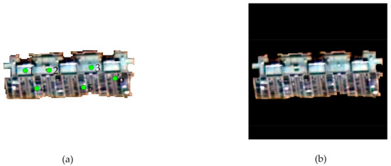
Figure 1.
An example of an image object: (a) the original image object; (b) the post-processing image object.
3.2. Architecture of the Designed Hybrid Model
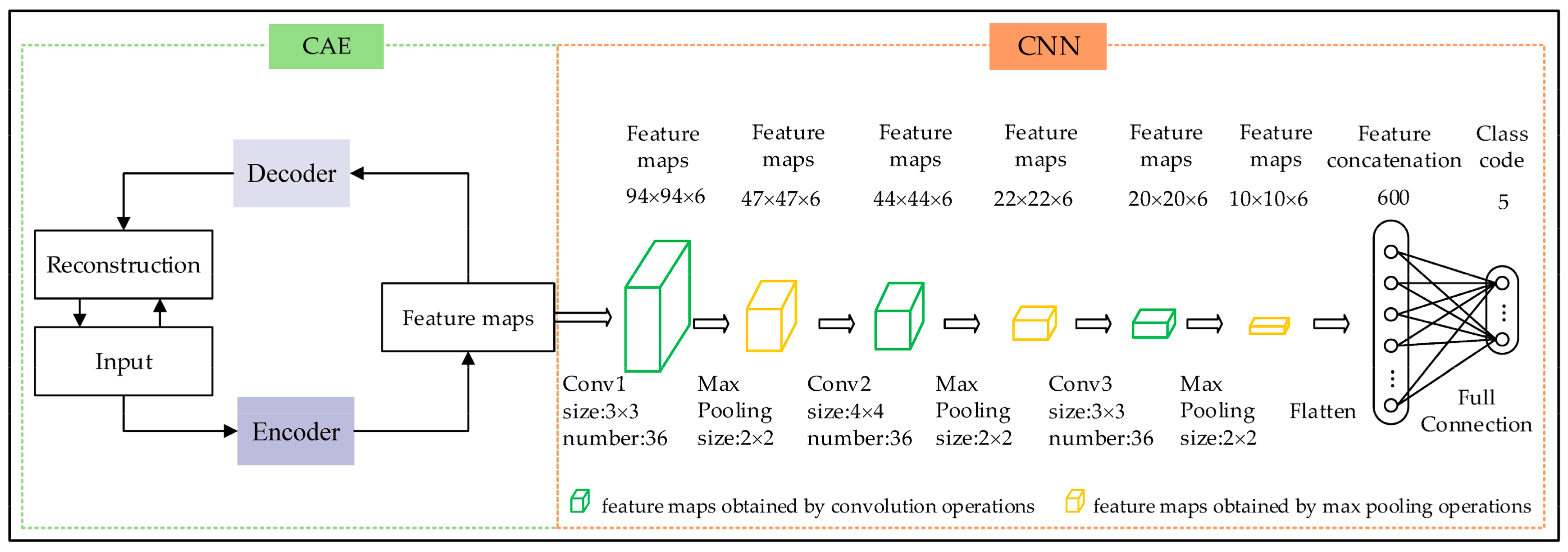
The proposed hybrid deep neural network model based on CAE and CNNs in object-oriented remote sensing classification (referred to as the CAE_CNN model) includes two steps. The first step requires training of the object-oriented remote sensing dataset without class information supervision based on the designed CAE model to extract feature maps and reduce the dimensionality of the data. The second step involves using the extracted feature maps as the inputs for the designed CNN model, which can then be classified.
The designed CAE model includes an encoder part and a decoder part. The encoder part includes a convolutional layer and a max pooling layer. The decoder part contains a deconvolution layer and an up-max pooling layer (layers are ascertained after repeated experiments).
The designed CNN model contains four layers with weights, including three convolutional layers and a fully-connected layer. The max pooling layer follows each convolutional layer.
The architecture of the CAE_CNN model can be seen in Figure 2 below.
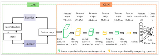
Figure 2.
Architecture of the CAE_CNN model (the green layers represent the feature maps obtained by convolution operations, and the yellow layers represent the feature maps obtained by max pooling operations).
4. Feature Extraction Based on the CAE Model
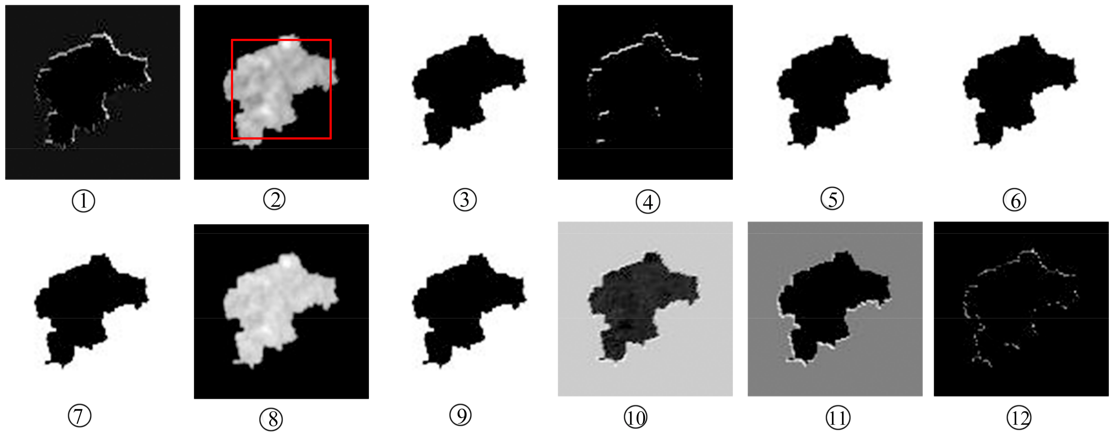
In this paper, the feature extraction and data dimension reduction of remote sensing image objects are carried out using the CAE; however, the number of extracted feature maps is difficult to determine and has a crucial impact on the classification results. In this case, we set the number to 12 to ensure that the data quality of the feature maps remains consistent with the original image. Figure 3 shows that an information redundancy phenomenon occurs between feature maps. Therefore, 12 feature maps should be grouped to eliminate redundant information and determine a more reasonable number of feature maps. The redundancy elimination method is as follows:
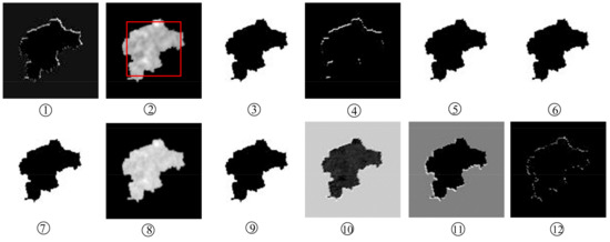
Figure 3.
Example of feature maps (the red box in feature map ② represents a central 53 × 53 grid).
In the central area of a 53 × 53 matrix of feature maps, the texture features of each feature map are compared and analysed based on entropy, energy, and inverse difference moment indicators derived from a grey-level co-occurrence matrix [32,33,34].
Sample 177 and its feature maps are shown as an example in Figure 3 below.
The change in each indicator is shown in Figure 4.

Figure 4.
Variation of each indicator.
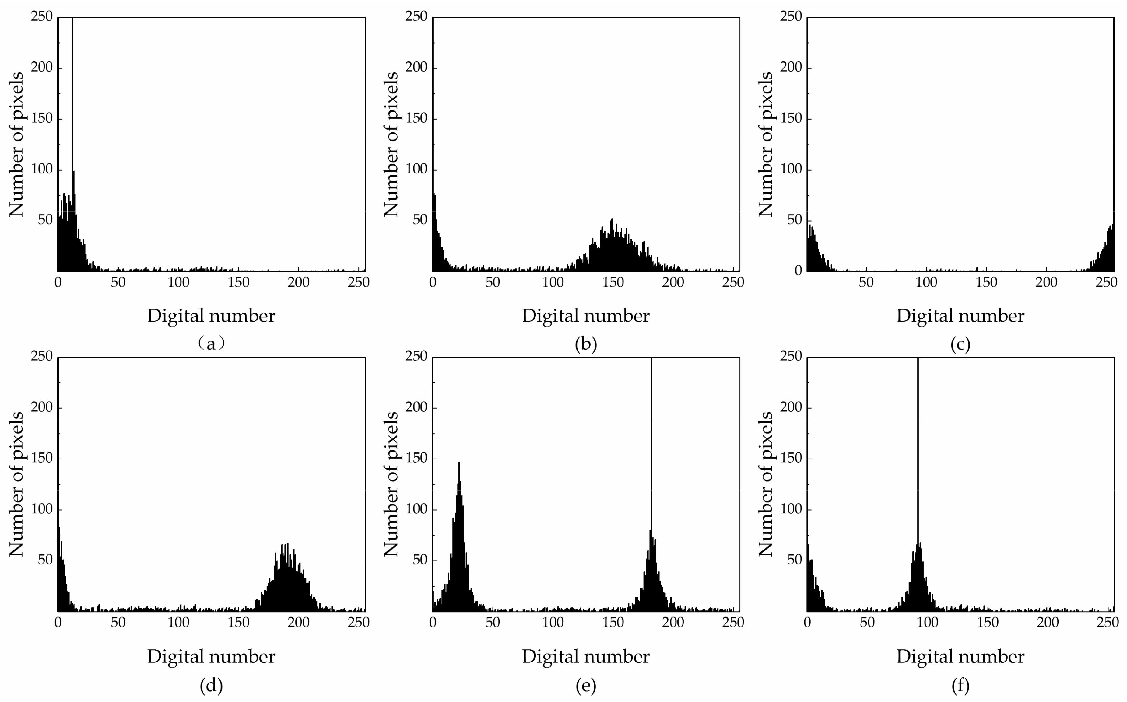
If the entropy value difference is less than 0.1, the maps are considered similar and can be grouped together. According to the graph, the entropy of feature maps 1, 4, and 12 is similar; therefore, the maps can be grouped together. The entropy values of feature maps 3, 5, 6, 7, and 9 are also similar, so these maps can be aggregated into a second group. The difference in entropy values of the other feature maps is greater, thus, each of these maps represents its own group. Therefore, there is information redundancy among 12 feature maps, and it is more effective to use 6 sets of feature maps instead of 12 feature maps. Next, based on the grey histogram (Figure 5) of each feature map, the information contained in each feature map is described.

Figure 5.
Grey histograms ((a–f) represent the grey histograms of feature maps 1, 2, 3, 8, 10, and 11, respectively. The grey histograms of feature maps 5, 6, 7, and 9 are similar to the grey histogram of feature map 3; and the grey histograms of feature maps 4 and 12 are similar to the grey histogram representing feature map 1.).
The entropy of feature maps 2 and 8 is 1.70 and 1.19, respectively. The energy of these feature maps is 0.31 and 0.47, respectively. The inverse difference moment of the feature maps is 0.93 and 0.94, respectively. These differences indicate that feature maps 2 and 8 have very rich and unique texture information. The grey histogram also shows that they have different spectral features, which are beneficial to classify.
The entropy of the feature maps numbered 1, 4, and 12 is almost 0, while the energy and inverse difference moments of these are close to 1, which indicates that the local areas of these maps lack variability and have no texture information. The grey histograms (4, 12, and 1 are similar) show that, in addition to the black background and the subject, some sporadic grey points constitute the subject’s contour, revealing obvious shape characteristics that are beneficial to classify.
The entropy, energy, and inverse difference moments of feature maps 3, 5, 6, 7, and 9 range from 0.75–0.85, 0.50–0.55, and 0.965–0.982, respectively. Although there is no texture information on the subject, where the external edge of the subject’s silhouette forms a point cloud through the convolution operation with rich texture information, the grey histograms (5, 6, 7, 9, and 3 similar) show that there is a clear distinction between the main body and the background. These features also have shape characteristics that are helpful to classify.
The entropy, energy, and inverse difference moments of feature maps 10 and 11 range from 0.25–0.6, 0.45–0.50, and 0.75–0.982, respectively, which suggests weaker texture information. Compared with the grey histograms of the other feature maps, 10 and 11 both have special and different spectral characteristics, which are beneficial to classify.
Therefore, there is redundancy among the 12 feature maps, and they are aggregated into 6 groups according to the minimum similarity principle. The different feature map groups reflect the different characteristics of the objects in those groups, which are beneficial to classify.
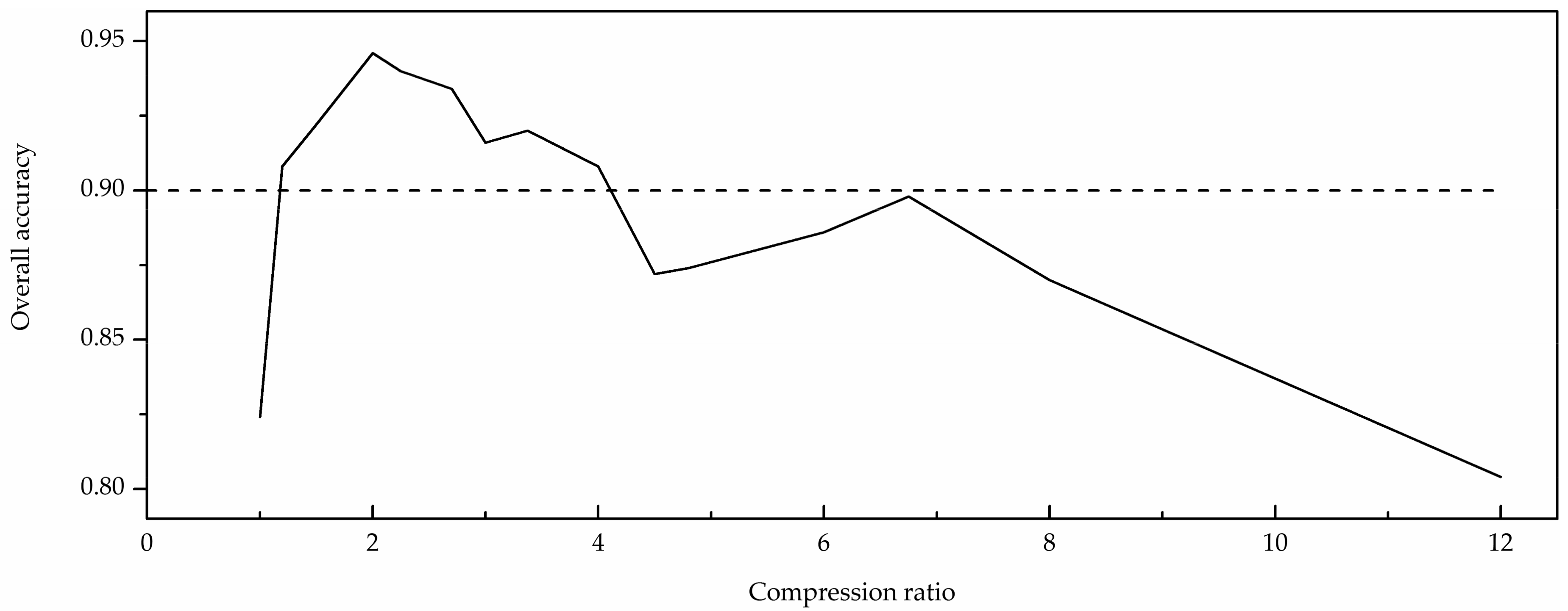
In addition to the number of feature maps, the size of the feature map is also an important factor that affects classification. The most ideal condition is that the process of extracting a feature map not only maintains the inherent information, but also reduces redundancy. The compression ratio can be used as an important indicator to evaluate the quality of the compressed image [35]. Through analysis of experiments using a variety of feature maps (as shown in Figure 6), classification accuracy reaches a maximum when the compression ratio is 2 and the size of the feature map is determined according to the principle.

Figure 6.
Overall accuracy with the compression ratio change.
5. Parameters of the CAE_CNN Model
The size of remote sensing objects is 192 × 192 × 3 according to the established parameter determination methods within the designed CAE model (proposed in Section 4). The number of feature maps is 6, and the compression ratio is 2. Thus, the size of the input feature maps of the designed CNN model is 96 × 96 × 6 and the number of feature maps is maintained at 6.
For the designed CNN model, the number of layers was ascertained after repeated experiments. Three convolutional layers were determined to be optimal, and it is important to employ small kernels for convolutional layers, so the kernel size of the first convolutional layer was established at 3 × 3. This corresponds to a 3 × 3 pixel area within the feature maps, which is equivalent to a ground area of 3 m × 3 m. This scale is more conducive to extracting spatial and spectral features from each image. The kernel sizes of the other two convolutional layers were established following the same principle; the number of kernels for each convolution layer is the product of the number of input feature maps (n) and the number of output feature maps (m). These kernels are divided into m groups, and each group has n kernels. Each kernel of each group is convolved with the corresponding input feature map, the results of which add up to an output feature map. Finally, the m feature maps were obtained. Common max pooling was used for the pooling layers; due to the limited size of the sample set, the neuron count of fully-connected layer must be less than 1000 in order to ensure a relatively good classification accuracy. Thus, the pooling layers were designed to be 2 × 2, which prevented over-fitting and ensures the efficiency of the network.
The rectified linear units (RELU) were applied to the output of every convolutional layer. The softmax classification method was applied to the full connection layer connected to the class code. The image objects were sampled uniformly from the whole training set in mini-batches of 10. The Adaptive Moment Estimation (Adam) method was adapted to optimize the model. Default settings for Adam are learning rate = 0.001, β1 = 0.9, β2 = 0.999, and epsilon = 10−8.
6. Results and Discussion
The study area used was in Hangzhou City. The remote sensing image is a Worldview II image with 8 multispectral bands and a panchromatic band. To integrate the advantages of multispectral and panchromatic images, the images were fused first. Because of the high correlation among the various bands, bands 1, 4, and 8, which had a low correlation, were selected as the best band combination for use in this study. A correlation analysis was performed to determine this result. Then, the sample set was obtained using the method proposed in Section 3. The training set contained 2000 samples and the testing set included 500 samples, including roads, forests, green space, water bodies, and residences.
To verify the validity and rationality of the CAE_CNN model, three experiments were carried out. The first experiment utilized the proposed CAE_CNN model to classify the remote sensing objects. The second experiment took the input, encoder, and feature maps module in the CAE of Figure 2 and connected the layer that produces feature maps to Conv1 of the CNN in Figure 2. We used the softmax classifier and trained the resulting network with supervision directly; this model is referred to as the CAE_SMX model. The third experiment analysed different pure CNN architectures to classify the original image objects and resulted in the selection of the best one; the resulting model contained nine layers with weights, including eight convolutional layers and a fully-connected layer. The structure is more complicated than the CAE_CNN model (as shown in Figure 7). This model is referred to as the Best_CNN model.

Figure 7.
Architecture of the Best_CNN model (the green layers represent the feature maps obtained by convolution operations, and the yellow layers represent the feature maps obtained by max pooling operations).
The three experiments were evaluated based on the overall accuracy, temporal efficiency, and dependency of the labelled samples.
6.1. Overall Accuracy of the Different Models
As shown in Table 2, Table 3 and Table 4, the overall accuracy of the CAE_CNN model is 0.944, which is higher than that of the CAE_SMX model (overall accuracy of 0.20) and the Best_CNN model (overall accuracy of 0.916). The classification accuracy of each category based on the CAE_CNN model is higher than or close to 90%. These results show that the CAE_CNN model has a significant advantage in object-oriented remote sensing classification compared to the CAE_SMX and Best_CNN models.

Table 2.
The confusion matrix of the CAE_CNN model.

Table 3.
The confusion matrix of the CAE_SMX model.

Table 4.
The confusion matrix of the Best_CNN model.
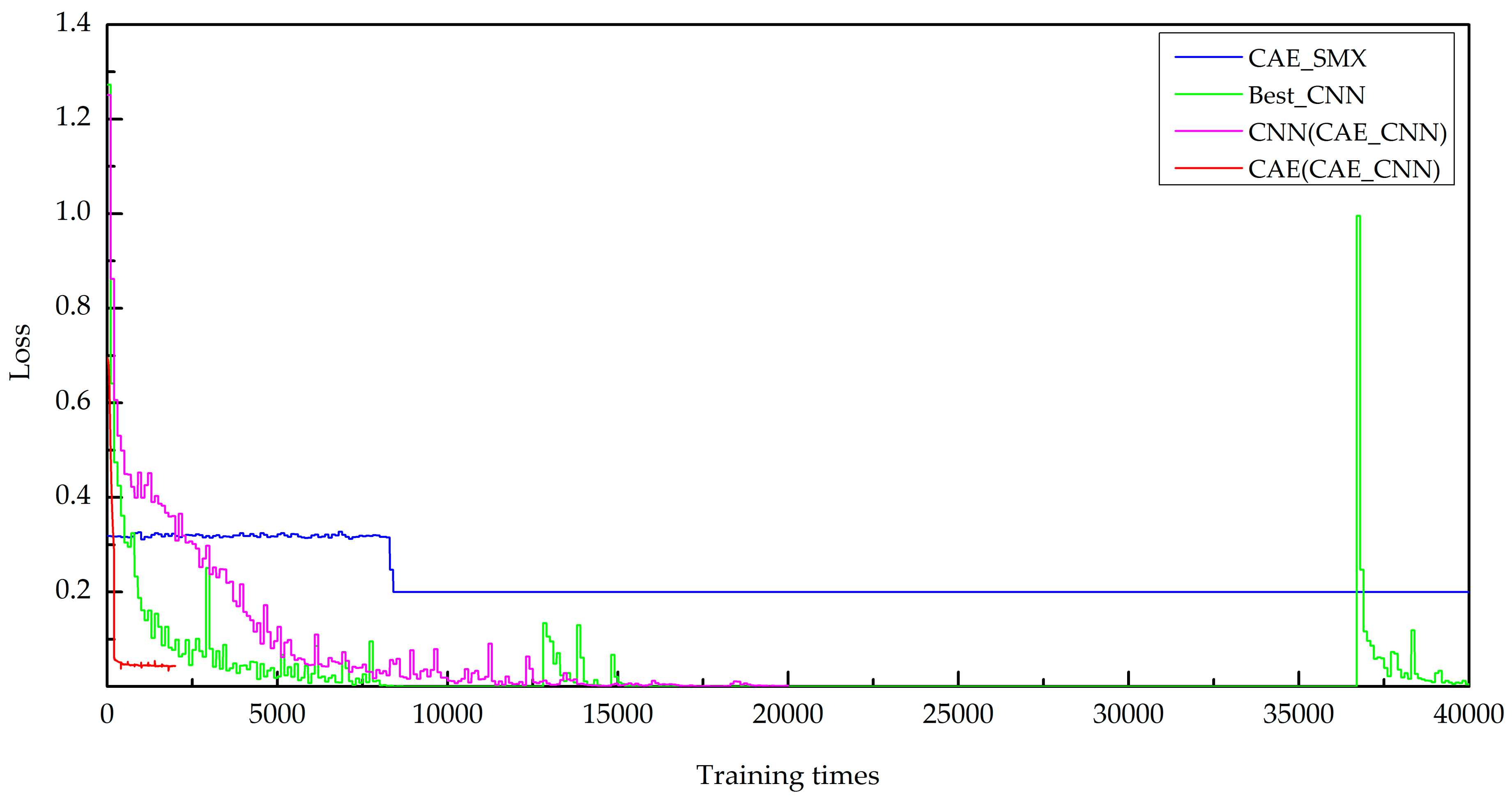
The loss function values of the CAE part have reached 0.0435 (as shown by the red line in Figure 8), which indicates that the feature maps extracted using the CAE are very effective and accurately represent the original image. Nevertheless, the overall accuracy of the CAE_SMX model is still only 0.2. These results indicate that the CAE is suitable for feature extraction and data dimension reduction but not direct classification.
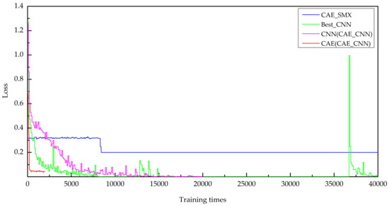
Figure 8.
Loss function values during model training.
The overall accuracy of the Best_CNN model is 0.916; this is not a relatively good accuracy, which indicates that the CNN has difficulty in achieving high accuracy results when classifying original objects directly, and the accuracy of the training set of the Best_CNN model reaches 0.998, indicating that the model is overfitted trained on the given data.
This analysis indicates that the CAE_CNN model combines the advantages of both the CAE and CNN to accurately classify the data, and the CAE_CNN model can overcome the problem that it is easy for traditional CNNs to fall into over-fitting to some extent in the case of limited numbers of labelled samples.
6.2. Temporal Efficiency of Different Models
As shown in Figure 8, when the number of training times reaches approximately 400, the loss function value of the CAE part of the CAE_CNN model is less than 0.05. The loss function value of the CNN part of the CAE_CNN model occurs during a descending state in the training process and a total of 22,000 training times is required for the CAE_CNN model. However, the loss function value of the CAE_SMX model vacillates between 0.2 and 0.4 before the number of training times reaches 8,340, and there is no decreasing trend until the number of training runs reaches 40,000. The loss function value of the Best_CNN model also occurs during a descending state in the training process; however, it fluctuates when the number of training runs is between approximately 36,000 and 37,000, and a total of 40,000 training times is required. These results show that the CAE_CNN model is much more efficient than the CAE_SMX model and Best_CNN model.
In general, the CAE_CNN model can significantly improve the classification accuracy and temporal efficiency of the classification process of object-oriented remote sensing images compared to the pure CAE model and the pure CNN model.
6.3. Dependence on Labelled Samples
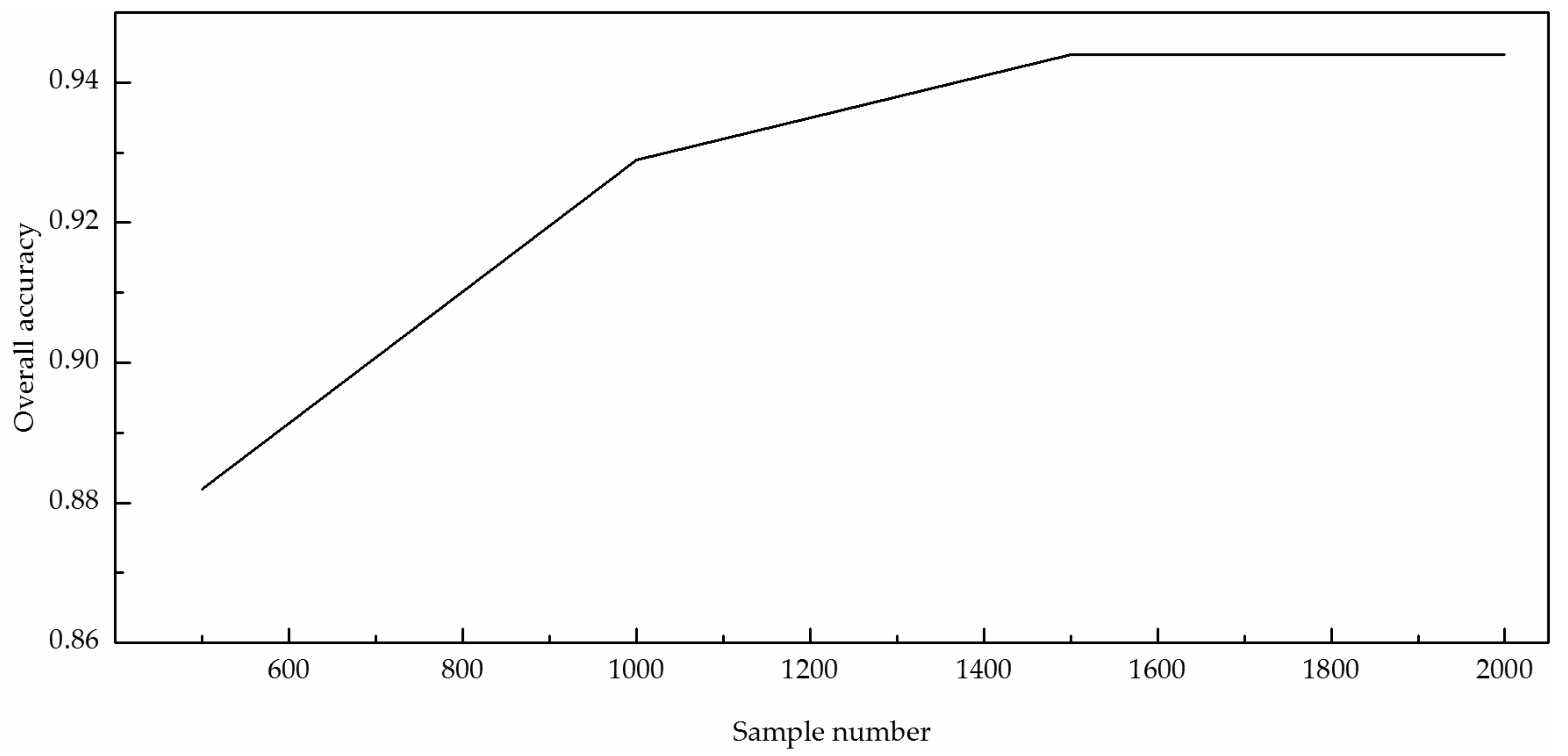
The CAE_CNN model structure is simple and requires fewer labelled samples. To verify that the CAE_CNN model can decrease the dependence of labelled samples, we trained the network using the same number of iterations by reducing the number of training set samples gradually and applied the classification to the same testing set. The results are shown in Figure 9.

Figure 9.
Classification accuracy with decreasing training set size.
As shown in Figure 9, the CAE_CNN model can still achieve a classification accuracy above 0.93 when the number of training sets is reduced to 1000, and the accuracy remains higher than the classification accuracy of the Best_CNN model, even while the training set of the Best_CNN model has 2000 samples. The results show that the CAE_CNN model can effectively reduce the use of manually labelled samples and thus the cost of manually marking samples.
As shown in Table 5, the number of parameters utilized drops from 5780 in the Best_CNN model to 4247 in the CAE_CNN model, while the number of parameters in the fully-connected layer remains similar. The number of parameters in the convolution layer decreases from 2895 to 1242 because the number of convolutional layers is reduced from 8 to 3; that is to say, the CAE_CNN model needs fewer parameters to extract features, so the CAE_CNN model can reduce its dependence on the number of labelled samples.

Table 5.
The number of parameters of the models.
In summary, the hybrid deep neural network model is able to achieve a higher efficiency and can significantly improve the accuracy of remote sensing image classification by taking advantage of a simpler structure. Furthermore, the number of labelled samples required is greatly reduced, which suggests that the interference of the subjectivity inherent in experts’ domain classification on the classification accuracy can be overcome to some extent.
7. Conclusions
A hybrid network design strategy for remote sensing classification is proposed to address the lack of a widely accepted remote sensing deep neural network model caused by the inability to establish a standard remote sensing sample dataset from imagery developed using different remote sensing data formats and researchers’ different classification requirements. Remote sensing imagery features are enhanced and data redundancy can be reduced using a convolutional auto-encoder. Then, those feature maps which reflect the essential information of the remote sensing data can be used as inputs into a convolutional neural network. This study demonstrates that the strategy not only improves image classification efficiency and accuracy, but also greatly reduces the number of labelled samples required. The strategy proposed has produced a viable and effective deep neural network design method for object-oriented remote sensing classification. In a future study, the authors will apply the proposed model to a broader range of data to establish a more universal model and find a more accurate and efficient way to determine the channel and scale of the output feature maps of the CAE.
Supplementary Materials
The following are available online at www.mdpi.com/1999-4893/11/1/9/s1.
Acknowledgments
This work was supported by the Wuhan Science and Technology Plan Program under Grant 2016010101010023, the CRSRI Open Research Program under Grant CKWV2015242/KY, the National Natural Science Foundation of China under Grant 41571514, and the National Key R&D Program of China under Grant 2017YFB0503700.
Author Contributions
Wei Cui and Qi Zhou conceived the original idea for the study, analyzed the experiment results, and revised the manuscript; Qi Zhou performed the experiments and wrote the manuscript; Zhendong Zheng analyzed the data. All authors read and approved the submitted manuscript.
Conflicts of Interest
The authors declare no conflict of interest.
References
- Bengio, Y. Learning Deep Architectures for AI. Found. Trends Mach. Learn. 2009, 2, 1–127. [Google Scholar] [CrossRef]
- Kavukcuoglu, K.; Sermanet, P.; Boureau, Y.L.; Gregor, K.; Lecun, Y. Learning convolutional feature hierarchies for visual recognition. In Proceedings of the International Conference on Neural Information Processing Systems, Vancouver, Canada, 6–9 December 2010; pp. 1090–1098. [Google Scholar]
- Hu, W.; Huang, Y.Y.; Wei, L.; Zhang, F.; Li, H.C. Deep convolutional neural networks for hyperspectral image classification. J. Sens. 2015, 2, 1–12. [Google Scholar] [CrossRef]
- Yue, J.; Zhao, W.Z.; Mao, S.J.; Liu, H. Spectral–spatial classification of hyperspectral images using deep convolutional neural networks. Remote Sens. Lett. 2015, 6, 468–477. [Google Scholar] [CrossRef]
- Lee, H.; Kwon, H. Contextual deep CNN based hyperspectral classification. In Proceedings of the IEEE International Geoscience and Remote Sensing Symposium, Beijing, China, 10–15 July 2016; p. 1. [Google Scholar]
- Han, X.B.; Zhong, Y.F.; Zhao, B.; Zhang, L.P. Scene classification based on a hierarchical convolutional sparse auto-encoder for high spatial resolution imagery. Int. J. Remote Sens. 2017, 38, 514–536. [Google Scholar] [CrossRef]
- Zhang, F.; Du, B.; Zhang, L.P. Scene classification via a gradient boosting random convolutional network framework. IEEE Trans. Geosci. Remote Sens. 2016, 54, 1793–1802. [Google Scholar] [CrossRef]
- Dstl Satellite Imagery Competition, 1st Place Winner’s Interview: Kyle Lee. Available online: http://blog.kaggle.com/2017/04/26/dstl-satellite-imagery-competition-1st-place-winners-interview-kyle-lee/ (accessed on 12 October 2017).
- Ronneberger, O.; Fischer, P.; Brox, P. U-Net convolutional networks for biomedical image segmentation. In Proceedings of the Medical Image Computing and Computer-Assisted Intervention-MICCAI, Munich, Germany, 5–9 October 2015; pp. 234–241. [Google Scholar]
- Baatz, M.; Schäpe, A. Multiresolution Segmentation: An optimization approach for high quality multi-scale image segmentation. Angew. Geogr. Informationsverarbeitung 2000, 12–23. [Google Scholar]
- Zhang, H.; Liu, X.Y.; Yang, S.; Yu, L.I. Retrieval of remote sensing images based on semisupervised deep learning. J. Remote Sens. 2017, 21, 406–414. [Google Scholar]
- Yang, N. Feature Selection for Object-oriented Classification of High Resolution Remote Sensing Images. Master’s Thesis, Xi’an University of Science and Technology, Xi’an, China, July 2012. [Google Scholar]
- Hinton, G.E.; Osindero, S.; Teh, Y.W. A fast learning algorithm for deep belief nets. Neural Comput. 2006, 18, 1527–1554. [Google Scholar] [CrossRef] [PubMed]
- Simonyan, K.; Zisserman, A. Very deep convolutional networks for large-scale image recognition. arXiv, 2015; arXiv:1409.1556. [Google Scholar]
- He, K.; Zhang, X.Y.; Ren, S.Q.; Sun, J. Deep residual learning for image recognition. In Proceedings of the IEEE Conference on Computer Vision and Pattern Recognition, Las Vegas, NV, USA, 27–30 June 2016; pp. 770–778. [Google Scholar]
- Szegedy, C.; Liu, W.; Jia, Y.Q.; Sermanet, P.; Reed, S.; Anguelov, D.; Erhan, D.; Vanhoucke, V.; Rabinovich, A. Going deeper with convolutions. In Proceedings of the IEEE Conference on Computer Vision and Pattern Recognition, Boston, MA, USA, 7–12 June 2015; pp. 1–9. [Google Scholar]
- Szegedy, C.; Vanhoucke, V.; Ioffe, S.; Shlens, J.; Wojna, Z. Rethinking the inception architecture for computer vision. In Proceedings of the IEEE Conference on Computer Vision and Pattern Recognition, Las Vegas, NV, USA, 27–30 June 2016; pp. 2818–2826. [Google Scholar]
- Szegedy, C.; Ioffe, S.; Vanhoucke, V.; Alemi, A. Inception-v4, inception-resnet and the impact of residual connections on learning. In Proceedings of Proceedings of the Thirty-First AAAI Conference on Artificial Intelligence, San Francisco, CA, USA, 4–9 February 2017. [Google Scholar]
- Chollet, F. Xception: Deep learning with depthwise separable convolutions. arXiv, 2017; arXiv:1610.02357. [Google Scholar]
- Krizhevsky, A. Learning Multiple Layers of Features from Tiny Images. Master’s Thesis, University of Toronto, ON, Canada, April 2009. [Google Scholar]
- Deng, J.; Wei, D.; Richard, S.; Li, L.J.; Li, K.; Li, F.F. Imagenet: A large-scale hierarchical image database. In Proceedings of the IEEE Conference on Computer Vision and Pattern Recognition, Miami, FL, USA, 20–25 June 2009; pp. 248–255. [Google Scholar]
- Lin, T.Y.; Maire, M.; Belongie, S.; Hays, J.; Perona, P.; Ramanan, D.; Dollár, P.; Zitnick, C.L. Microsoft coco: common objects in context. In Proceedings of the European Conference on Computer Vision, Zurich, Switzerland, 6–12 September 2014; pp. 740–755. [Google Scholar]
- Hinton, G.E.; Salakhutdinov, R.R. Reducing the dimensionality of data with neural networks. Science 2006, 313, 504–507. [Google Scholar] [CrossRef] [PubMed]
- Tan, S.Q.; Li, B. Stacked convolutional auto-encoders for steganalysis of digital images. In Proceedings of the Asia-Pacific Signal and Information Processing Association Summit and Conference, Chiang Mai, Thailand, 9–12 December 2014; pp. 1–4. [Google Scholar]
- Geng, C.; Song, J.X. Human Action recognition based on convolutional neural networks with a convolutional auto-encoder. Proceedings of 2015 5th International Conference on Computer Sciences and Automation Engineering, Sanya, China, 14–15 November 2015. [Google Scholar]
- Masci, J.; Meier, U.; Cireşan, D.; Schmidhuber, J. Stacked Convolutional auto-encoders for hierarchical feature extraction. In Proceedings of the International Conference on Artificial Neural Networks, Espoo, Finland, 14–17 June 2011; pp. 52–59. [Google Scholar]
- Zayene, O.; Seuret, M.; Touj, S.M.; Hennebert, J.; Ingold, R.; Ben Amara, N.E. Text detection in Arabic news video based on SWT operator and convolutional auto-encoders. In Proceedings of the Document Analysis Systems, Santorini, Greece, 11–14 April 2016; pp. 13–18. [Google Scholar]
- Han, X.B.; Zhong, Y.F.; Zhao, B.; Zhang, L.P. Unsupervised hierarchical convolutional sparse auto-encoder for high spatial resolution imagery scene classification. In Proceedings of the International Conference on Natural Computation, Zhangjiajie, China, 15–17 August 2015; pp. 42–46. [Google Scholar]
- Maimaitimin, M.; Watanabe, K.; Maeyama, S. Stacked convolutional auto-encoders for surface recognition based on 3d point cloud data. Artif. Life Robot. 2017, 22, 259–264. [Google Scholar] [CrossRef]
- Ioffe, S.; Szegedy, C. Batch normalization: accelerating deep network training by reducing internal covariate shift. In Proceedings of the International Conference on Machine Learning, Lille, France, 6–11 July 2015; pp. 448–456. [Google Scholar]
- Alberti, M.; Seuret, M.; Ingold, R.; Liwicki, M. What You Expect is NOT What You Get! Questioning Reconstruction/Classification Correlation of Stacked Convolutional Auto-Encoder Features. arXiv, 2017; arXiv:1703.04332. [Google Scholar]
- Haralick, R.M. Texture features for image classification. IEEE Trans. Syst. Man Cybern. 1973, 6, 610–621. [Google Scholar] [CrossRef]
- Park, B.; Lawrence, K.C.; Windham, W.R.; Chen, Y.R.; Chao, K. Discriminant analysis of dual-wavelength spectral images for classifying poultry carcasses. Comput. Electron. Agric. 2002, 33, 219–231. [Google Scholar] [CrossRef]
- Liu, Q.; Liu, X.P.; Zhang, L.J.; Zhao, L.M. Image texture feature extraction & recognition of Chinese herbal medicine based on gray level co-occurrence matrix. Adv. Mater. Res. 2013, 605–607, 2240–2244. [Google Scholar] [CrossRef]
- Jiang, J.; Reddy, M. Open-loop rate control for JPEC-LS near lossless image compression. Electron. Lett. 1999, 35, 465–466. [Google Scholar] [CrossRef]
© 2018 by the authors. Licensee MDPI, Basel, Switzerland. This article is an open access article distributed under the terms and conditions of the Creative Commons Attribution (CC BY) license (http://creativecommons.org/licenses/by/4.0/).


