Abstract
We present an algorithm selection framework based on machine learning for the exact computation of treewidth, an intensively studied graph parameter that is NP-hard to compute. Specifically, we analyse the comparative performance of three state-of-the-art exact treewidth algorithms on a wide array of graphs and use this information to predict which of the algorithms, on a graph by graph basis, will compute the treewidth the quickest. Experimental results show that the proposed meta-algorithm outperforms existing methods on benchmark instances on all three performance metrics we use: in a nutshell, it computes treewidth faster than any single algorithm in isolation. We analyse our results to derive insights about graph feature importance and the strengths and weaknesses of the algorithms we used. Our results are further evidence of the advantages to be gained by strategically blending machine learning and combinatorial optimisation approaches within a hybrid algorithmic framework. The machine learning model we use is intentionally simple to emphasise that speedup can already be obtained without having to engage in the full complexities of machine learning engineering. We reflect on how future work could extend this simple but effective, proof-of-concept by deploying more sophisticated machine learning models.
1. Introduction
1.1. The Importance of Treewidth
The treewidth of an undirected graph , denoted , is a measure of how “treelike” it is [1]. Trees have treewidth 1 and the treewidth of a graph can be as large as . The concept of treewidth is closely linked to that of a tree decomposition of G, which is the arrangement of a set of subsets of V into a tree backbone, such that certain formal criteria are satisfied; these are described in the preliminaries. The width of the tree decomposition is equal to the size of its largest subset, minus 1 and is the minimum width, ranging over all possible tree decompositions of G [2]. In recent decades treewidth has attracted an immense amount of attention, due to the observation that many NP-hard problems on graphs become polynomial-time solveable on graphs of bounded treewidth. This is because, when a tree decomposition of width t is available, it is usually possible to organise dynamic programming algorithms in a hierarchical way such that the intermediate lookup-tables consulted by the dynamic programming, have size that is bounded by a function of t [3]. In fact, because of this many NP-hard problems on graphs can actually be solved in time , where and f is a computable (typically exponential) function that depends only on . We say then that the problem is fixed parameter tractable (FPT) with respect to . For this reason, treewidth has become a cornerstone of the parameterized complexity literature, which advocates a more fine-grained approach to running time complexity than the traditional approach of expressing worst-case running times purely as a function of the size of the input [4].
Given its relevance as a `gateway to tractability’, treewidth has attracted enormous interest not just from the combinatorial optimisation and theoretical computer science communities but also from many other domains such as artificial intelligence (particularly Bayesian inference and constraint satisfaction: see Reference [5] for a highly comprehensive list), computational biology [6] and operations research [7]. Unfortunately, computing the treewidth (equivalently, a minimum-width tree decomposition) is NP-hard [8]. This does not nullify its usefulness, however. Alongside practical heuristics (see e.g., References [9,10]) there is an extensive literature on computing the treewidth of a graph exactly, in spite of its NP-hardness. Some of these results have a purely theoretical flavour, most famously in Reference [11] but there has also been a consistent stream of research on computing treewidth exactly in practice. Such practical algorithms have an interesting history. Until a few years ago, progress had been somewhat incremental; see References [12,13] for representative articles from this period. However, in 2016 the Parameterized Algorithms and Computational Experiments (PACE) treewidth challenge, an initiative of the parameterized complexity community to promote the development of practically efficient algorithms, stimulated a major breakthrough. The positive-instance driven dynamic programming approach pioneered by Tamaki [14] allowed the treewidth to be computed exactly for many graphs that had hitherto been considered out of range [14,15]. This 2017 edition of PACE subsequently yielded an additional hundred-fold speed-up over PACE 2016 results [16].
Following the advances triggered by PACE 2016 and Tamaki’s approach, there are now a number of highly advanced exact treewidth solvers, several of which we will encounter later in this article. When studying these solvers we observed that, once the solving time rose above a few seconds, no single solver universally dominated over (i.e., ran more quickly than) all the others. This led us to the following insight: if we could decide, on a graph-by-graph basis, which solver will compute the treewidth of the graph most quickly, we could contribute to a further reduction in the time required to compute treewidth by selecting this fastest algorithm. Traditionally, such an approach would involve a blend of comparing worst-case time complexities, analysing the `inner workings’ of the algorithms and an ad-hoc exploration of which types of graphs do and do not solve quickly on certain algorithms. Such a process, however, is time-consuming, requires algorithm-specific knowledge and may have limited efficacy due to the opaqueness of the algorithmic approaches used and/or highly complex correlations between input characteristics and algorithmic performance. Hence the question: can we, as far as possible, automatically learn the relative strengths of a set of algorithms? This brings us to the domain of machine learning [17] and machine learning-driven algorithm selection in particular.
We note that, although interest has peaked in recent years due to the emergence of data science, there is already a quite extensive literature on the use of machine learning in combinatorial optimisation and integer linear programming in particular (see e.g, References [18,19,20]). In addition to algorithm selection, which we will elaborate upon below, this literature focuses on topics such as classification of instances by difficulty [21], running time regression [22,23] and learning to branch [24,25,26]. We refer to References [22,27] for excellent surveys of the area and References [28,29,30] for some recent case-specific applications in operations research.
1.2. Algorithm Selection
The algorithm selection problem was initially formulated by Rice [31] to deal with the following question: given a problem instance and a set of algorithms, which algorithm should be selected to solve the instance? The simplest answer to this question is dubbed the `winner takes all’ approach—all candidate algorithms’ performance is measured on a set of problem instances and only the algorithm with the best average performance is used. However, there is always a risk that the algorithm that is best on average will be a sub-optimal choice for many specific instances.
Conversely, the ideal solution to the problem would be an oracle predictor that always knows which algorithm is best for any instance. In practice, it is rarely possible to create such a predictor. Instead, researchers strive to heuristically approximate an oracle. In 2003 Leyton-Brown et al. provided the first proof-of-concept of per-instance selection [32]. Since then, notable applications and successes include SAT solvers [33,34], classification [35], probabilistic inference [36], graph coloring [37], integer linear programming [38] and many others. For a thorough history of the development and applications of algorithm selection, the reader is referred to Kerschke et al. [39].
1.3. Our Contribution
Although machine learning has been applied to learn desirable characteristics of a given set of tree decompositions [40] (with a view to speeding up dynamic programming algorithms that then run over the tree decompositions), algorithm selection has not been applied to the computation of treewidth itself. This paper sets out to fill that gap by demonstrating a working algorithm selection framework for the problem. Specifically, we use standard, “out of the box” techniques from machine learning to train a classifier which subsequently decides, on a graph by graph basis, which out of a set of state-of-the-art exact treewidth solvers will terminate fastest. The exact treewidth algorithms were all submissions to Track A of the aforementioned PACE 2017 tournament. The resulting hybrid algorithm significantly outperforms any single one of the algorithms in isolation. We also investigate the features (i.e., measurable characteristics) of problem instances and solvers that make some (graph, algorithm) pairings better than others. The data used to train the classifier has been made publicly available at github.com/bslavchev/as-treewidth-exact. We feel that the combination of treewidth and the machine learning approach to algorithm selection is particularly timely, given that they both fit into the wider movement towards fine-grained, multivariate analysis of running-time complexity. In order to keep the exposition compact and accessible for a wider audience we have deliberately chosen for a stripped-down machine learning framework in which we only use a generic, easy-to-compute set of features and a small number of pre-selected classifiers. As we explain in the section on future work, more features, classifiers and analytical techniques can certainly be explored in the future. However, the take-away message for this article is that machine learning-driven algorithm selection can already be effective without having to resort to highly sophisticated machine learning frameworks.
The structure of this paper is as follows: Section 2 will formally define treewidth and the algorithm selection problem. Section 3 will describe the graph features, treewidth solvers and machine learning models that we used. Section 4 will present the datasets used, the experiments conducted and their results. Section 5 will further analyse the experiment results, while Section 6 contains a discussion of the insights that the research has yielded. Finally, Section 7 reflects on possible future work and the trend towards the incorporation of machine learning techniques within combinatorial optimisation.
2. Preliminaries
2.1. Tree Decompositions and Treewidth
Formally, given an undirected graph , a tree decomposition of G is a pair where X is a set whose individual elements are subsets of V called bags and T is a tree whose nodes are the subsets . Additionally, the following three rules hold:
- The union of all bags equals V, i.e., every vertex of the original graph G is in at least one bag in the tree decomposition.
- For every edge in G, there exists a bag X that contains both u and v, i.e., both endpoints of every edge in the original graph G can be found together in at least one bag in the tree decomposition.
- If two bags and both contain a vertex v, then every bag on the path between and also contains v.
The treewidth of a tree decomposition is the size of the largest bag in the decomposition, minus one and the treewidth of a graph G is the minimum width ranging over all tree decompositions of G [2].
2.2. Algorithm Selection
The Algorithm Selection problem, as formulated by Rice [31], deals with the following question: Given a problem instance and a set of algorithms, which algorithm should be selected to solve the instance? Rice identified four defining characteristics of the algorithm selection problem:
- the set of algorithms A,
- the instances of the problem, also known as the problem space P,
- measurable characteristics (features) of a problem instance, known as the feature space F,
- the performance space Y.
The selection procedure S is what connects these four components together and produces the final answer—given an instance , S selects from A an algorithm based on the features that has, in order to maximize the performance .
3. Methodology
3.1. Features
Algorithm selection is normally based on a set of features that are extracted from problem instances under the assumption that those features contain signal for which algorithm to select. The choice of features is, of course, subjective. To enhance generality and avoid circularity, we deliberately avoided selecting features based on specific knowledge of how the treewidth algorithms operate. To that end, we extracted thirteen features from each of the graphs, listed below. These are very standard summary statistics of graphs, which are a subset of the features used by Reference [37] where algorithm selection was used to tackle the NP-hard graph colouring problem. More specifically, we selected these features because they are trivial to compute, ensuring that the feature extraction phase of our hybrid algorithm requires only a negligible amount of time to execute. The remaining features used by Reference [37] are more complex and time-consuming to compute, requiring non-trivial polynomial-time algorithms to approximate a number of other graph parameters, several of which are themselves NP-hard to compute. Compared to many machine learning frameworks, our selected subset is a fairly small set of features: it is more common to start with a very large set of features and then to progressively eliminate features that do not seem to contain signal. Nevertheless, as we shall see in due course, our parsimonious choice of features seems well-suited to the problem at hand.
- 1:
- number of nodes:v
- 2:
- number of edges:e
- 3,4:
- ratio:,
- 5:
- density:
- 6–13:
- degree statistics: min, max, mean, median, , , variation coefficient, entropy.
For brevity, the features , and variation coefficient will be referred to as q1 (first quartile), q3 (third quartile) and variation in the rest of this paper. We note that there are some mathematical correlations in the above features, particularly between and . We keep both to align with Reference [37], where both features were also used but also because we wish to defer the question of feature correlations and significance to our post-facto feature analysis later in the article. There we observe that leaving out exactly one of and in any case does not improve performance. Other correlations in the features are more indirect and occur via more complex mathematical transformations. There is no guarantee that the classifiers we use can easily `learn’ these complex correlations, which justifies inclusion. It is also useful to keep all 13 features to illustrate that careful pre-processing of features, which can be quite a complex process, is not strictly necessary to obtain a powerful hybrid algorithm.
3.2. Treewidth Algorithms
The treewidth implementations and algorithms used were submissions to Track A of the 2017 Parameterized Algorithms and Computational Experiments (PACE) competition [16]. All solvers used are listed below with a brief description and a link to where the implementation can be accessed. We emphasise that, where solvers have multiple functionalities, we used used them in exact mode. That is, we ask the solver to compute the true treewidth of the graph, not a heuristic approximation of it.
- tdlib, by Lukas Larisch and Felix Salfelder, referred to as tdlib. This is an implementation of the algorithm that Tamaki proposed [14] for the 2016 iteration of the PACE challenge [15], which itself builds on the algorithm by Arnborg et al. [8]. Implementation available at github.com/freetdi/p17
- Exact Treewidth, by Hisao Tamaki and Hiromu Ohtsuka, referred to as tamaki. Also an implementation of Tamaki’s algorithm [14]. Implementation available at github.com/TCS-Meiji/PACE2017-TrackA
- Jdrasil, by Max Bannach, Sebastian Berndt and Thorsten Ehlers, referred to as Jdrasil [41]. Implementation available at github.com/maxbannach/Jdrasil
Tamaki’s original 2016 implementation [14] was initially considered but later excluded due to being dominated by other algorithms, that is, there was no problem instance where it was the fastest solver.
3.3. Machine Learning Algorithms
We start by introducing two standard techniques from machine learning. Both these techniques generate, after analysing training data, a classifier: in our case, an algorithm to which we input the 13 features of the input graph and which then outputs which of the three treewidth solvers to run on that graph.
Decision Trees are a widely-used model for solving classification problems [42]. The model works by partitioning the training dataset according to the features of each instance, with each partition being assigned one of the target labels. The partitioning is done in steps—first, the entire dataset is partitioned and then each of the resulting partitions may be further partitioned recursively, until a certain condition is met. The resulting model can be expressed hierarchically as a rooted tree, where every node represents a partition and every edge represents a partitioning rule based on instance features. Then, classifying an instance is as simple as starting at the root node and following the path that the instance takes according to its features and the partitioning rules it encounters. The leaf node in which the instance ends up determines the label that it should be assigned. A comprehensive introduction to decision trees is due to Kotsiantis [42]. Decisions trees are popular due to their interpretability. Some of their disadvantages include a propensity for overfitting through building too-complex trees, as well as the possibility for small changes in the training dataset to produce radical differences in the resulting tree [43].
Random Forest is also a widely-used model for solving classification problems, based on decision trees [44]. Essentially, a Random Forest is an ensemble model that uses a majority-voting system between multiple decision trees to classify instances. The trees themselves are also built according to special rules—a detailed explanation of those and Random Forests in general is due to Liaw et al. [44]. Random Forests exhibit strong predictive performance and resistance to over-fitting.
Due to their strong predictive performance, our primary results use Random Forests to learn the mapping from graphs to algorithms. However, compared to a single decision tree, Random Forest classifiers can be difficult to interpret. For this reason we also consider classification based on a single decision tree, which in this article turns out to have marginally lower predictive power but allows us to analyse and interpret the sequence of decisions taken to map graphs to algorithms. Once built, the computational time required to execute our classifiers is negligible.
3.4. Reflections on the Choice of Machine Learning Model
First, we note that in addition to Random Forests and decision trees the machine learning literature encompasses a wide range of other classifiers which could be used to select the best algorithm. It is not the purpose of this article to undertake comparative analysis of all these different classifiers in order to identify the best classifier, although this is something that future work could certainly explore. Rather, we wish to demonstrate that, armed with a sensible choice of classifier, algorithm selection can already outperform the original algorithms in isolation. Random Forests are renowned for their predictive power (see e.g., the discussions in References [37,45]), motivating our choice in this case. For completeness we did also try a Support Vector Machine (SVM) model [46], which attempts to classify instances through the use of separating hyperplanes but due to very weak performance in preliminary experiments we did not explore it further.
Second, we remark that our current model—selecting the fastest algorithm—is only one of many possibilities for estimating performance. For example, one could try a regression-based approach whereby a mathematical model is trained that estimates the actual running time of an algorithm on a given input graph. Then, the (estimated) running times of the three algorithms could be computed and compared, allowing us a more detailed insight into the relative performance of the algorithms. Such an approach certainly has its merits and would also obviate the need for moderate difficulty filtering, which we describe in the next section. However, we defer this to future work, since our simple classification model already proves to be highly effective, even with the aforementioned filtering technicality. Also, there are quite some complexities and choices involved in modelling and learning the running times of sophisticated algorithms, which at this stage would over-complicate the exposition and introduce an extra layer of parameter estimation.
We return to both these points in the future work section.
4. Experiments and Results
4.1. Datasets
The dataset we used is composed of a multitude of publicly available graph datasets—this section will provide a list of all datasets used and where they can be found. Some needed to be converted to the PACE treewidth format from their original format—those are marked with an asterisk (*) in the list below. Additionally, the list will also provide a shorthand name for every dataset. Datasets used are:
- PACE 2017 treewidth exact competition instances, referred to as ex. Available at github.com/PACE-challenge/Treewidth-PACE-2017-instances
- PACE 2017 bonus instances, referred to as bonus. Available at github.com/PACE-challenge/Treewidth-PACE-2017-bonus-instances
- Named graphs, referred to as named. (These are graphs with special names, originally extracted from the SAGE graphs database). Available at github.com/freetdi/named-graphs
- Control flow graphs, referred to as cfg. Available at github.com/freetdi/CFGs
- PACE 2017 treewidth heuristic competition instances, referred to as he. Available at github.com/PACE-challenge/Treewidth-PACE-2017-instances
- UAI 2014 Probabilistic Inference Competition instances, referred to as uai. Available at github.com/PACE-challenge/UAI-2014-competition-graphs
- SAT competition graphs, referred to as sat_sr15. Available at people.mmci.uni-saarland.de/ hdell/pace17/SAT-competition-gaifman.tar
- Transit graphs, referred to as transit. Available at github.com/daajoe/transit_graphs
- PACE 2016 treewidth instances [15], referred to as pace2016. Available at bit.ly/pace16-tw-instances-20160307
- Asgeirsson and Stein [47]*, referred to as vc. Available at ru.is/kennarar/eyjo/vertexcover.html
- PACE 2019 Vertex Cover challenge instances*, referred to as vcPACE. Available at pacechallenge.org/files/pace2019-vc-exact-public-v2.tar.bz2
- DIMACS Maximum Clique benchmark instances*, referred to as dimacsMC. Available at iridia.ulb.ac.be/~fmascia/maximum_clique/DIMACS-benchmark
In total, 30,340 graphs from these datasets were used.
4.2. Experimental Setup
The features described in Section 3.1 were extracted from all graphs. All algorithms described in Section 3.2 were run on all graphs from Section 4.1.
The three exact algorithms tested in this research output a solution as soon as they find one and then terminate. However, a limit of 30 min run time was imposed to keep tests within an acceptable time frame; this is the same as the time limit used in the PACE 2017 competition. If an algorithm was terminated due to going above the time limit, it was presumed to have failed to find a solution. For each run, we recorded whether the algorithm terminated within the time limit, the running time (if it did) and the treewidth of the solution. Recording the treewidth is not strictly necessary, since we are primarily interested in which algorithm terminates most quickly but it is useful auxiliary information and we have made it publicly available. All experiments were conducted on Google Cloud Compute virtual machines with 50 vCPUs and 325GB memory. Since all algorithm implementations used are single-threaded, fifty experiments were run in parallel. Where necessary (e.g., Java-based solvers), each experiment was allocated 6.5GB of heap space.
The extracted features and experimental results were combined into a single dataset, in order to train the machine learning models. There were 162 graphs on which attempting to run a solver or the feature extractor would cause either the process or the machine where the process was running to crash. Most of the time, these graphs came from datasets that were not meant for exact treewidth computation, such as sat_sr15, he and dimacsMC (Section 4.1) and were therefore too big. For instance, all graphs of the sat_sr15 dataset were too hard for any solver to terminate. For an even more extreme example, graphs 195 through 200 of the PACE 2017 Heuristic Competition dataset were all too big for our feature extractor to load them into memory, with graph 195 being the smallest of them at 1.3 million vertices and graph 200 being the biggest at 15.5 million. These graphs are three orders of magnitude larger than the graphs the implementations were built to work on—the biggest graph from the PACE 2017 Exact Competition dataset is graph number 198, which has 3104 vertices. Other errors included unusual yet trivial cases like the graph collect-neighbor_collect_neighbor_init.gr from the dataset cfg, which only contained one vertex and which broke assumptions of both our feature extractor and the solvers we used. All such entries were discarded from the dataset. An additional 680 entries were discarded because no solver managed to obtain a solution on them in the given time limit—presumably those problem instances were too hard. The resulting dataset contained a total of 29,498 instances.
In the course of preliminary experiments, it was discovered that the dataset we assembled required some further pre-processing. When each graph in the dataset was assigned a label corresponding to the exact algorithm that found a solution the fastest, a very large class imbalance was detected—tdlib was labeled the best algorithm for about 99% (29,234) of instances; Jdrasil—for under 0.2% (55); and tamaki—for about 0.7% (209). Under these circumstances, an algorithm selection approach could trivially achieve 99% accuracy by simply always selecting tdlib. To create genuine added value above this trivial baseline, we imposed additional rules in order to re-balance the dataset towards graphs that are neither too easy, nor too hard; we call these graphs of moderate difficulty. Graphs were considered not of moderate difficulty if either all algorithms found a solution quicker than some lower bound (i.e., the graph is too easy), or all algorithms failed to find a solution within the allotted time (i.e., the graph is too hard). The reasoning behind this approach is that if algorithms’ run times lie outside of the defined moderate area, there is little gains to be made with algorithm selection anyway. If a graph is too easy, a comparatively weak algorithm can still solve it quickly; if a graph is too hard, there simply is no “correct" algorithm to select. Formally, if is the lower bound, is the allotted time (upper bound) and is the run time of algorithm A on graph G, then if holds, G will be excluded.
Three different lower bounds were used—1, 10 and 30 s—and graphs that passed the conditions were stored in datasets A, B and C, respectively. (For the upper bound, we used the time-out limit of 30 min). This necessitates us making a distinction between source datasets and filtered datasets—the source datasets are those publicly available datasets that we started with; the filtered datasets are the sum of all graphs from all source datasets which passed through the respective filter. Table 1 breaks down how many graphs from each source dataset remained in each filtered dataset.

Table 1.
The total number of graphs per source dataset and the number of those graphs in filtered datasets A, B and C (see Section 4.1 and Section 4.2 for clarification).
The same label-assigning procedure described above was repeated. The resulting class distributions are shown in Table 2. Afterwards, Random Forest models were trained using the Python machine-learning package scikit-learn [48], using all default settings except for allowing for up to 1000 trees in the forest. Both Leave-One-Out (LOO) cross-validation and 5-fold cross-validation were used in order to decrease the importance of randomness in the train-test split. 5-fold cross validation was repeated 100 times with different random seeds for the same purpose; at the end, the results from all 100 runs were averaged. These two cross-validation methods produced virtually identical results, hence we only present the results for LOO cross-validation. The results presented are for the entire dataset. Our algorithm selector is evaluated based on its predictions for each graph when it was in the test set—that is, a model is never evaluated on a graph that it has been trained on. We deemed the usage of a hold-out set unnecessary, as no hyper-parameter optimisation took place. (For readers not familiar with these technical machine learning terms, we refer to survey literature such as Tsamardinos et al. [49]).
Table 2.
Number of graphs, within each dataset, for which the given algorithm was fastest (see Section 4.1 and Section 4.2).
An additional model was trained on Dataset B, using a single CART decision tree as a classifier and 50% of the data as a training set. The purpose of this model was not to optimise predictive performance but interpretability, as a Decision Tree model is significantly easier to interpret than a Random Forest model. We hoped that this interpretation would provide insight into what makes solvers good on some instances and bad on others. Dataset B was chosen due to having the best class distribution, with no clearly best algorithm.
An experiment using Principal Component Analysis (PCA) for dimensionality reduction was also undertaken on Dataset B. The purpose was to evaluate to what extent the feature set can be shrunk without significant loss of performance and potentially to provide insight into feature importance through examination of the principal components.
Reflections on filtering. Before turning to the results, we wish to reflect further on moderate difficulty filtering, described above. Recall: graphs which are not of moderate difficulty, are those where all the solvers terminated extremely quickly (i.e., more quickly than the lower bound) or all the solvers exceeded the upper bound (here: exceeded 30 min of run time, that is, timed out). As mentioned earlier, we originally introduced this filtering after observing heavy skew in the initial dataset. We did not know a priori what the `correct’ lower bound should be, which is why we tried three different values (1, 10, 30 s) (Note that, once the bound is chosen, the Random Forest classifier can be trained on our data in less than a minute, although cross-validation takes longer). As our results show, this filtering is sufficient to obtain a hybrid algorithm that clearly outperforms the individual algorithms. Interestingly, the filtering also mirrors our practical experience of solving NP-hard problems exactly. That is, many different algorithms can solve easy instances of NP-hard problems within a few seconds but beyond this running times of algorithms tend to increase dramatically and relative efficiencies of different algorithms become more pronounced: one algorithm might take seconds, while another takes hours or days. Once inputs are eliminated that are far too hard for any existing exact algorithm to solve, we are left with inputs that are harder than a certain triviality threshold but not impossibly hard—and it is particularly useful to be able to distinguish between algorithmic performance in this zone. A second issue concerns the choice of lower bound. If we wish to use the hybrid algorithm in practice, by training it on newly gathered data, what should the lower bound be? If we do not have any information at all concerning the underlying distribution of running times—which will always be a challenge for any machine learning model—we propose training using a lower bound such as 1 or 10 s. Unseen graphs which are moderately difficult (subject to the chosen bound) will utilise the classifier in the region it was trained for. Others will be solved very quickly by all solvers—a running time of at most 10 s is, for many NP-hard problems, very fast—or all solvers will time out, and then it does not, in practice, matter which algorithm the model chose. In the future work section we consider alternatives to moderate difficulty filtering.
4.3. Experimental Results
This section is divided into five subsections where each of the first three subsections covers the results of experimenting on one of the three datasets generated by setting a different lower bound for algorithms’ run time, as described in Section 4.2. The hybrid algorithm—essentially, the mapping from graph to algorithm that is prescribed by the trained classifier—will be compared against the solvers and against an `oracle’ algorithm, which is a hypothetical hybrid algorithm that always selects the best solver. Three performance metrics will be used:
- Victories. A `victory’ is defined as being (or selecting, in the case of the hybrid algorithm or the oracle algorithm) the fastest algorithm for a certain graph.
- Total run time on the entire dataset.
- Terminations. A `termination’ is defined as successfully solving the given problem instance within the given time. No regard is given to the run-time, the only thing that matters is whether the algorithm managed to find a solution at all.
Please refer to Figure 1 for detailed results from these three experiments. We note that the running times for the hybrid algorithm do not include the time to execute the Random Forest classifier. This is acceptable because in the context of the experiments its contribution to the running time is negligible: approximately a hundredth of a second for a single graph.
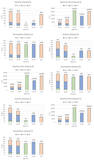
Figure 1.
Experimental results using Leave-One-Out cross-validation. Each chart presents the results from the experiment on one of the three datasets (A, B and C) based on one of the three performance metrics (victories, total run time and terminations). For the Oracle and Hybrid algorithms, results are not presented as an aggregate of all solver choices—instead, each solver’s contribution to each performance metric is presented separately (see Section 4.2 and Section 4.3). Total running times are measured in seconds.
The fourth subsection covers the experiment conducted on Dataset B with a decision tree classifier, while the fifth subsection covers the Principal Component Analysis experiment.
4.3.1. Dataset A
(The information in this subsection can also be found in Figure 1; similarly for Datasets B and C). The hybrid algorithm selected the fastest algorithm on 1025 out of 1162 graphs, whereas the best individual solver (tdlib) was fastest for 898. The hybrid algorithm’s run time was 87,500 s, while the overall fastest solver (tamaki) required 137,447 s and the perfect algorithm—54,810 s). The hybrid algorithm terminated on 1145 out of the 1162 graphs, whereas the best solver (tamaki) terminated on 1115.
4.3.2. Dataset B
The hybrid algorithm selected the fastest algorithm on 326 out of 427 graphs, whereas the best individual solver (tdlib) was fastest for 192. The hybrid algorithm’s run time was 82,085 s, while the overall fastest solver (tamaki) required 135,935 s and the perfect algorithm—54,466 s. The hybrid algorithm terminated on 413 out of the 427 graphs, whereas the best solver (tamaki) terminated on 380.
4.3.3. Dataset C
The hybrid algorithm selected the fastest algorithm on 261 out of 337 graphs, whereas the best individual solver (tamaki) was fastest for 168. The hybrid algorithm’s run time was 80,697 s, while the overall fastest solver (tamaki) required 134,910 s and the perfect algorithm—54,060 s. The hybrid algorithm terminated on 323 out of the 337 graphs, whereas the best solver (tamaki) terminated on 290.
4.3.4. Dataset B—Decision Tree
A decision tree was trained with the default scikit-learn settings but it was too large to interpret, having more than 40 leaf nodes. We optimised the model’s hyper-parameters until we obtained a model that was small enough that it could be easily interpreted, without sacrificing too much accuracy. The final model was built with the following restrictions: any leaf node must contain at least 2 samples; the maximum depth of the tree is 3; a node is not allowed to split if its impurity is lower than 0.25.
The resulting hybrid algorithm’s performance was deemed satisfactorily close to the Random Forest selector we trained on the same dataset. The decision tree selected the fastest algorithm on 151 out of 214 graphs, whereas the Random Forest model selected the fastest for 153. The decision tree selector’s run time was 54,017 s, while the Random Forest selector required 55,696 s. The decision tree selector terminated on 202 out of the 214 graphs, whereas the Random Forest selector terminated on 201.
4.3.5. Dataset B—Principal Component Analysis
Principal Component Analysis with three components was applied to the dataset and used to train a Random Forest classifier, which was trained and evaluated in the same way as the other Random Forest models. The three components cumulatively explained about 90% of the variance in the data; for a detailed breakdown, please refer to Table 3. The trained model had an accuracy of about 73% compared to the baseline model’s accuracy of 76.5%. While the loss of accuracy is small, our drop-column feature analysis in Section 5 shows many sets of three features that can be used to build a model of similar or higher accuracy.
Table 3.
The individual components in the Principal Component Analysis. Each row refers to one of the three components. The leftmost column shows how much of the total variance of the data is explained by that component; all other columns show how the respective feature is factored into the component.
5. Analysis
In this section, the experimental results and the machine learning models behind them are analysed with the intention of deriving insights into why certain algorithm-graph pairings are stronger than others and to determine which features of a graph are the most predictive.
We begin by analysing the importance of features for a Random Forest model trained on 50% of Dataset B. We chose to train a separate model, instead of using one from our cross-validation, because those models are all trained on all but one samples. We chose that dataset because of its class distribution—the two solvers that are strong on average (tdlib and tamaki) have nearly equal results and the third solver (Jdrasil) is still best for a significant number of problem instances, unlike in Dataset A. This guarantees that the hybrid algorithm’s task is the hardest, as the trivial `winner-takes-all’ approach would be the least effective.
We used the feature importance functionality that is built into the scikit-learn package. The results are presented in Figure 2. The results indicate that almost all features are important for the classification and their importance varies within relatively tight bounds.
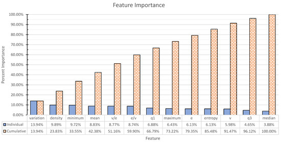
Figure 2.
Feature importance for the Random Forest model trained on Dataset B (Section 4.2). We refer the reader to Section 3.1 for the list of features used. Each bar indicates the fraction of impurity in the dataset that is removed by splits on the relevant feature in all trees of the model.
In order to gain further insight, we decided to exclude certain features from the dataset, retraining the model on the reduced dataset and measuring its accuracy against the baseline of the original full model, which is 76.5%. In order to obtain more statistically robust results, we made multiple runs of 10-fold cross-validation and kept their scores.
Afterwards, the scores were compared to the baseline of using all features using the Wilcoxon Signed-Rank Test with an alpha of 0.05.
At first, we attempted excluding single features. We did 10-fold cross-validation 50 times for every excluded feature. No result was statistically significantly different from the baseline.
Next, we attempted excluding two features at a time. Again, we did 10-fold cross-validation 50 times for every excluded set of features. Two pairs of features obtained a statistically significant worse accuracy score—variation and minimum degree, as well as variation and entropy.
Finally, we attempted excluding three features at a time. This time, we did 10-fold cross-validation only 5 times, as here the computational cost of doing otherwise was prohibitive. While there were 14 sets of features that led to significantly worse scores, the magnitude of the change was rather small—the worst performance was 74.5% and was achieved by removing minimum degree, maximum degree and variation. Of note is also the fact that 13 of 14 sets contained at least two of these same features and one set contained only one of them.
Since removing features seemed to provide us with little insight, we attempted another approach—removing all features except for a small number of designated features. Then we repeated the same procedure—we retrained the model on the reduced dataset and measured its accuracy against the original model. Again, we did 10-fold cross-validation a multitude of times. We began by only selecting one feature to retain, repeating the training 50 times. The feature minimum degree emerged as a clear winner, having 72% accuracy. We highlight the fact that by removing three features at a time, we only managed to lower the accuracy to about 74.5%, while a model with only one feature successfully reached 72%.
Next, we selected pairs of features to keep and did 10-fold cross-validation 50 times. 7 sets of features performed at least as well as the original model. All of them contained variation and/or maximum degree.
Finally, we selected sets of 3 features to keep and did 10-fold cross-validation 5 times. More than 50 sets of features performed at least as well as the original model. Notably, despite the previously demonstrated importance of variation, minimum degree and maximum degree, adding all three of them produced results that were around the middle of the pack at 74.5%. However, a large majority of the best results contained at least one or more often two of those features.
All experiments also showed models that surpassed the performance of the benchmark model, reaching 78.5% by only adding mean, variation and maximum degree—compared to 76.5% for the original model. Naturally, we view such results with caution. They could well be the result of chance, especially seeing as how we use no validation set—however, another possibility is that the classifiers can be more efficiently trained on smaller subsets of features.
The frequency with which the features variation, minimum degree and maximum degree appear in our analysis indicates that they carry some critically important signal that the classifier needs in order to be accurate. However, it appears that one or two of the features are sufficient to reproduce the signal and adding the third one does not help much.
We also attempted to determine feature importance by examining the Decision Tree model that was built for Dataset B (Figure 3). Our analysis ignores nodes that offer under 50% accuracy and nodes that contain very few (less than four) samples, as those are deemed not to bring a significant amount of insight to the analysis.
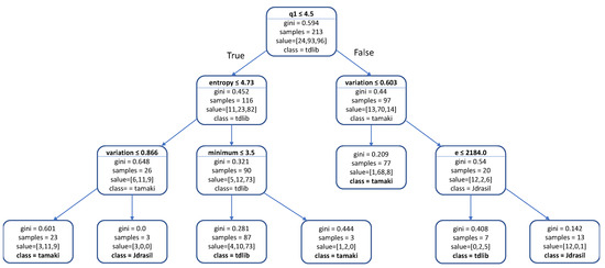
Figure 3.
The CART Decision Tree trained on Dataset B. Each rectangle represents a node in the tree. The first line in each internal node indicates the condition according to which that node splits instances. In leaf nodes, this line is omitted, as no split is executed there. Each internal node’s left child pertains to the subset of instances that met the condition, whereas the right child pertains to those that did not meet the condition. The next line describes the node’s Gini impurity, which is the probability that a randomly chosen element from the set would be incorrectly labeled if its label was randomly drawn from the distribution of labels in the subset. The next line shows how many graphs are in the subset that the node represents, while the following line shows how many instances of each class are in that subset, with the three values corresponding to Jdrasil, tamaki and tdlib, respectively. The last line shows the class which is the most represented in the subset, which is also the class that the Decision Tree would assign to all instances in that subset.
The very first split in the model already provides a dramatic improvement in accuracy. Its left branch is heavily dominated by tdlib—after that split alone, selecting tdlib would be the correct choice about 70% of the time. On the right side of the split, a similar situation is observed with tamaki being the correct choice about 72% of the time. This shows that the first split, which sends to the left graphs where the first quartile of the degree distribution is smaller than or equal to 4.5, is very important for solvers’ performance. The first quartile being low is an indicator for a small or sparse graph and according to the model, tdlib’s performance on those is better, while tamaki seems to cope better with larger or denser graphs.
There are two paths that lead to Jdrasil being the correct label, both of which require that the variation coefficient feature is higher than a certain threshold, which is quite high (0.603 and 0.866). This leads us to believe that Jdrasil performs well on graphs where there is significant variation in the degree of all vertices. One of these paths also requires the graph to have more than 2184 edges or otherwise tdlib is selected instead. This again indicates that tdlib is better at solving smaller or sparser graphs, while Jdrasil can deal with variability in larger graphs too.
One thing worth highlighting is that tdlib also seems to excel on graphs where the degree distribution has a low first quartile and the minimum degree is low. This also confirms our belief that tdlib excels on smaller and sparser graphs.
6. Discussion
In this section, the experimental results and analysis are discussed and some general insights are derived. One such general insight is the relative unavailability of graph sets of moderate difficulty. Depending on the definition of `moderate’, only between 1 and 3 percent of the graphs we tested could be considered as such. A likely explanation for this is that most datasets were assembled before the 2016 and 2017 editions of the PACE challenge, which introduced implementations that were multiple orders of magnitude faster than what was previously available, which in turn rendered many instances too easy.
Moving to specific points, we start by noting the promising performance of our hybrid algorithm compared to individual solvers. Our experiments clearly demonstrate the strength of the algorithm selection approach, as it outperformed all solvers on all datasets and all performance metrics, even though our underlying machine learning model is (deliberately) simple. However, the comparison with an omniscient algorithm selector also demonstrates that there is room for improvement in our framework. Section 7 lays out some suggestions for how our work can be improved upon.
Next, we reflect on the question: which features of a problem instance are the most predictive? We utilised three different approaches to answering this question—measuring how much each feature reduces impurity in our Random Forest model on Dataset B, measuring the performance of models that were only trained on a subset of all features and analysing the Decision Tree model we trained on Dataset B. Overall, our three approaches provided different and sometimes conflicting insights but some insights were confirmed by multiple approaches. One such insight is that there do not seem to be critically important individual features, as it appears that many different features can carry the same information, partly or in whole, which makes determining their individual importance difficult.
Measuring the impurity reduction of all features indicated that all features have a positive contribution to prediction. The most important feature, degree variation coefficient, was only about 3.5 times more important than the least important feature, median degree. The overall distribution of feature importances is such that the most important five features together account for about 50% of the importance, while the remaining eight account for the rest. Our interpretation of these results is that they show all features being significant contributors and while there are features that are more important than others, there are no clearly dominant features that eliminate the need for others.
The feature removal analysis indicated that three features—variation, minimum degree and maximum degree—all seem to be related in that removing all of them significantly reduces performance and performance increases as more of them are added, until all three are added, which does not provide a significant improvement in performance. Our interpretation is that there is a predictive signal that is present only in those three features but any two of them are sufficient to reproduce it. Besides this insight, feature removal provided little that we could interpret and that was not in direct conflict with other parts of the same analysis.
The analysis of the Decision Tree model indicated that size, density and variability are the most important characteristics of a graph; however, those could be expressed through different numerical features. For instance, the first quartile of the degree distribution (q1), which could be an indicator for graph size or density, was by far the most predictive feature in our Decision Tree model. To make discussing this easier, we will separate the concepts characteristic and feature. Characteristics are a more general characteristic that can be represented by many different features; features are specifically the numbers we described in Section 3.1.
Combining the results from all three approaches is difficult, as they often conflict. However, the insight from the Decision Tree analysis that size, density and variability are the most important characteristics of a graph, no matter what specific numerical proxy they are represented by, is consistent with results from other analysis approaches. The feature removal analysis indicated that variation, minimum degree and maximum degree together carry an important signal—these features can be considered a proxy for size, density and variability. The impurity reduction results are also consistent with this, as they showed variation, density and minimum degree being the three most important features. The relative lack of importance stemming from which proxy is used for these characteristics of a graph is also demonstrated by q1—while that feature is by far the most important in the Decision Tree analysis, the other two analytical approaches did not show it being particularly important, as it was only seventh out of thirteen in impurity reduction and did not make even one appearance in the sets of important features that the feature removal analysis yielded.
Our experiments also yield some insights into the strengths and weaknesses of the solvers. One insight that becomes clear from the class distribution in both our unfiltered dataset and the three filtered datasets (as per Section 4.2) is that the solver tdlib is dominant on `easy’ graphs. In the unfiltered dataset, tdlib was the best algorithm for 97% of graphs which became progressively less with a higher lower bound being imposed on difficulty. At the lower bound of 30 s (Dataset A), tdlib was the best algorithm for 77% of graphs; at 10 s (Dataset B) that number went further down to 45%; and at 30 s (Dataset C) it was only 38%. Notably, tdlib kept the “most victories" title in the unfiltered dataset, Dataset A and Dataset B; however, in Dataset C, tamaki dethroned it with 49% versus 38%. Undeniably, going from a 97% dominance to no longer being the best algorithm as difficulty increases tells us something about the strengths and weaknesses of the solver. This is also confirmed by our analysis of the Decision Tree model, which clearly showed tdlib had an aptitude for smaller and sparser graphs.
Another insight is tamaki’s robustness. It is the best solver in terms of terminations and run time on all three datasets, despite not being the best in terms of victories on datasets A and B. Most interesting is tamaki’s time performance on Dataset A—while tdlib has more than four times as many victories on that dataset as tamaki does, tamaki’s run time is still about 30% better than tdlib’s. Our analysis of the Decision Tree model showed tamaki having an affinity for larger or denser graphs, complementing tdlib’s strength on smaller or sparser graphs. The weakness of tamaki on sparse graphs that we discover is consistent with the findings of the solver’s creator [14].
Finally, Jdrasil seemed to have a tighter niche than the other solvers—specifically, larger graphs with a lot of variability in their vertices’ degree. However, Jdrasil clearly struggles on most graphs, as evidenced by its always coming in last in our experiments on all datasets and all performance metrics.
Summarizing, our analysis suggests that the most important characteristics of a graph are size, density and variability and that when focussing on these characteristics the three algorithms have the following strengths: tdlib—low density and size; tamaki—high density and size, low variability; Jdrasil—high density and size, high variability.
7. Conclusions and Future Work
7.1. Conclusions
In this article, we presented a novel approach based on machine learning for algorithm selection to compute the treewidth of a graph. Given a set of algorithms and a set of features of a specific problem instance, our system predicts which algorithm is most likely to have the best performance, according to a previously learned classification model. For this purpose, 13 features of graphs were identified and used. To evaluate our approach, we compared three state-of-the-art solvers, our hybrid algorithm and a hypothetical, perfect `oracle’ algorithm selection system, on thirteen publicly-available graph datasets and three performance measures. Our intentionally stripped-down machine learning approach outperformed all individual solvers on all datasets and on all performance metrics, which clearly demonstrates its utility. However, the hypothetical perfect algorithm selector still significantly outperformed our approach, which indicates that there are further improvements to be made. Based on our results, we argued that size, density and degree variability are the most important characteristics of a graph that determine which algorithm would be fastest on it. We also identified specific solvers’ strengths and weaknesses based on these same characteristics.
7.2. Future Work
One weakness of our work is that algorithms were only run once on each graph, so any randomness in algorithms’ run time is completely unaccounted for—future work may try to alleviate that by running algorithms several times and obtaining a confidence interval on the run time. Another sensitive part of our experimental framework concerns the selection of the three running time lower bounds (1, 10 and 30 s) that defined our three moderately difficult datasets A, B and C. These choices echo the practical experience of many algorithm designers that, if an exponential-time algorithm takes more than a few seconds to terminate, the running time quickly explodes and the comparative efficiencies of the algorithms become more important. It would be interesting to try to place the selection of such lower bounds on a more formal footing; in some sense they capture an interesting `triviality threshold’ beyond which the performance of existing treewidth solvers starts to deviate in a practically significant way. Future work could also explore whether the moderate difficulty filtering can be removed altogether, obviating the need to select the lower bound during training. One logical step in this direction would be to switch from our `who wins?’ classification model, to a regression-based model which is capable of predicting the running time of individual algorithms (or some kind of weighted classification model which takes the margin of victory into account). The regression model(s) could be used to estimate the running time of the different treewidth solvers on a given input graph, the fastest solver would then be chosen and auxiliary sensitivity analysis such as the margin of victory would then also be immediately available. There has been some interesting work on running-time regression of this kind (see e.g., References [22,23,50]). Such an approach could be effective but it is non-trivial to learn the running times of sophisticated algorithms, particularly if—as in this case—it is unclear what type of mathematical function (modelling the running time) we are trying to learn or whether the same function is applicable to all the different solvers. Indeed, more experimental parameters will need to be estimated and tuned and when modelling running times some kind of context-sensitive choices seem unavoidable to ensure that the regression model focuses on running times of the appropriate order of magnitude. For example, in the present context it would be most important that the regression model predicts well when running times are seconds or minutes, not microseconds or years. In other words, it is possible that the parameter estimation inherent in our moderate difficulty filtering will re-emerge somewhere else in the regression model. Nevertheless we regard this as a very interesting route for future research.
Introducing more solvers could offer further improvement, as additional solvers might exhibit a different set of strengths and weaknesses which the algorithm selection approach can then exploit. Also, as already discussed in Section 6, using a larger and more diverse set of graphs to experiment on, with a focus on graphs that are neither too easy nor too hard for algorithm selection to be useful, could strengthen the research: given the advances of PACE 2016, there is an urgent need for new, more difficult (but not too difficult!) datasets. Following standard machine learning methodology, we could consider incorporating different/more features, experimenting with different classifiers and carefully optimising hyper-parameters.
In order to make such research easier, we have provided full access to the dataset we generated for this project. The dataset can be found on github.com/bslavchev/as-treewidth-exact.
More generally, we suggest a more thorough and rigorous analysis of feature importance (and their interactions). It would be fascinating to delve into the underlying mechanics of the three treewidth solvers (tdlib, tamaki, Jdrasil) to try to shed more light on why certain (graph, algorithm) pairings are superior to others and to analyse how different features of the graph contribute to the running times of the algorithms. It is highly speculative but perhaps such an analysis could help to identify new parameters which can then be analysed using the formal machinery of parameterized complexity. In this article we chose emphatically not to “open the black box” in this way, preferring instead to see how far a simple machine learning framework could succeed using generic graph features and without in-depth, algorithm-specific knowledge. Nevertheless, such an analysis would be a valuable contribution to the algorithm selection literature. (Beyond treewidth, it would be interesting to explore whether our simple machine learning framework can be effective, without extensive modification, in the computation of other NP-hard graph parameters.)
Finally we suggest the development of an easy-to-use software package that utilises our work and the state of the art in treewidth solvers to provide the best possible performance out of the box and to aid researchers and practitioners alike. Rather than re-inventing the wheel anew, it is probably wisest to integrate an algorithm selection framework into an existing general treewidth framework (such as the wider tdlib ecosystem, which is available at github.com/freetdi/tdlib), as it would provide numerous opportunities and benefits—for example, selecting not just solvers but also pre-processors and kernelisation algorithms for treewidth (see Reference [51] and the references therein) and using the results from pre-processors as features for the solver selection, among others. Such a framework could also incorporate advances in computing treewidth using parallel processing [52].
7.3. The Best of Both Worlds
As a final note, we view our work as part of the accelerating trend towards the use of machine learning to derive data-driven insights, which are then used to enhance the in-practice performance of combinatorial optimisation algorithms. The deepening synthesis between predictive and prescriptive analytics in operations research is also part of this trend. Combinatorial optimisation traditionally focusses on aggressively optimised algorithms, which are then analysed using worst-case, univariate complexity analysis. Apart from the simplest algorithms, such one-dimensional analyses cannot adequately capture the role of many implicit parameters in determining the running time of algorithms (and indeed, the emergence of parameterized/multivariate complexity is a formal reaction to this). Machine learning, although not the appropriate instrument for combinatorial optimisation per se, can fulfill a powerful role in automatically fathoming such implicit parameters.
Author Contributions
Conceptualization, B.S., E.M., S.K.; methodology, B.S., E.M.; software, B.S.; validation, B.S., E.M.; formal analysis, B.S., E.M., S.K.; investigation, B.S., E.M.; resources, B.S.; data curation, B.S., E.M.; Writing—Original draft preparation, B.S.; Writing—Review and editing, B.S., E.M. S.K.; visualization, B.S.; supervision, S.K.; project administration, S.K.
Funding
This research received no external funding.
Acknowledgments
The authors thank the two anonymous reviewers for constructive and insightful comments, and Bas Willemse for moral and practical support during the writing of the article.
Conflicts of Interest
The authors declare no conflict of interest.
References
- Diestel, R. Graph Theory (Graduate Texts in Mathematics); Springer: New York, NY, USA, 2005. [Google Scholar]
- Bodlaender, H.L. A tourist guide through treewidth. Acta Cybern. 1994, 11, 1. [Google Scholar]
- Bodlaender, H.L.; Koster, A.M. Combinatorial optimization on graphs of bounded treewidth. Comput. J. 2008, 51, 255–269. [Google Scholar] [CrossRef]
- Cygan, M.; Fomin, F.V.; Kowalik, L.; Lokshtanov, D.; Marx, D.; Pilipczuk, M.; Pilipczuk, M.; Saurabh, S. Parameterized Algorithms; Springer: Cham, Switzerland, 2015; Volume 4. [Google Scholar]
- Bannach, M.; Berndt, S. Positive-Instance Driven Dynamic Programming for Graph Searching. arXiv 2019, arXiv:1905.01134. [Google Scholar]
- Hammer, S.; Wang, W.; Will, S.; Ponty, Y. Fixed-parameter tractable sampling for RNA design with multiple target structures. BMC Bioinform. 2019, 20, 209. [Google Scholar] [CrossRef] [PubMed]
- Bienstock, D.; Ozbay, N. Tree-width and the Sherali–Adams operator. Discret. Optim. 2004, 1, 13–21. [Google Scholar] [CrossRef]
- Arnborg, S.; Corneil, D.G.; Proskurowski, A. Complexity of finding embeddings in a k-tree. SIAM J. Algeb. Discret. Methods 1987, 8, 277–284. [Google Scholar] [CrossRef]
- Strasser, B. Computing Tree Decompositions with FlowCutter: PACE 2017 Submission. arXiv 2017, arXiv:1709.08949. [Google Scholar]
- Van Wersch, R.; Kelk, S. ToTo: An open database for computation, storage and retrieval of tree decompositions. Discret. Appl. Math. 2017, 217, 389–393. [Google Scholar] [CrossRef]
- Bodlaender, H. A Linear-Time Algorithm for Finding Tree-Decompositions of Small Treewidth. SIAM J. Comput. 1996, 25, 1305–1317. [Google Scholar] [CrossRef]
- Bodlaender, H.L.; Fomin, F.V.; Koster, A.M.; Kratsch, D.; Thilikos, D.M. On exact algorithms for treewidth. ACM Trans. Algorithms (TALG) 2012, 9, 12. [Google Scholar] [CrossRef]
- Gogate, V.; Dechter, R. A complete anytime algorithm for treewidth. In Proceedings of the 20th conference on Uncertainty in artificial intelligence, UAI 2004, Banff, AB, Canada, 7–11 July 2004; AUAI Press: Arlington, VA, USA, 2004; pp. 201–208. [Google Scholar]
- Tamaki, H. Positive-instance driven dynamic programming for treewidth. J. Comb. Optim. 2019, 37, 1283–1311. [Google Scholar] [CrossRef]
- Dell, H.; Husfeldt, T.; Jansen, B.M.; Kaski, P.; Komusiewicz, C.; Rosamond, F.A. The first parameterized algorithms and computational experiments challenge. In Proceedings of the 11th International Symposium on Parameterized and Exact Computation (IPEC 2016), Aarhus, Denmark, 24–26 August 2016; Schloss Dagstuhl-Leibniz-Zentrum für Informatik: Wadern, Germany, 2017. [Google Scholar]
- Dell, H.; Komusiewicz, C.; Talmon, N.; Weller, M. The PACE 2017 Parameterized Algorithms and Computational Experiments Challenge: The Second Iteration. In Proceedings of the 12th International Symposium on Parameterized and Exact Computation (IPEC 2017), Leibniz International Proceedings in Informatics (LIPIcs), Vienna, Austria, 6–8 September 2017; Lokshtanov, D., Nishimura, N., Eds.; Schloss Dagstuhl–Leibniz-Zentrum fuer Informatik: Dagstuhl, Germany, 2018; Volume 89, pp. 1–12. [Google Scholar] [CrossRef]
- Jordan, M.I.; Mitchell, T.M. Machine learning: Trends, perspectives, and prospects. Science 2015, 349, 255–260. [Google Scholar] [CrossRef]
- Hutter, F.; Hoos, H.H.; Leyton-Brown, K. Automated configuration of mixed integer programming solvers. In Proceedings of the International Conference on Integration of Artificial Intelligence (AI) and Operations Research (OR) Techniques in Constraint Programming, Thessaloniki, Greece, 4–7 June 2019; Springer: Cham, Switzerland, 2010; pp. 186–202. [Google Scholar]
- Kruber, M.; Lübbecke, M.E.; Parmentier, A. Learning when to use a decomposition. In Proceedings of the International Conference on AI and OR Techniques in Constraint Programming for Combinatorial Optimization Problems, Padova, Italy, 5–8 June 2017; Springer: Cham, Switzerland, 2017; pp. 202–210. [Google Scholar]
- Tang, Y.; Agrawal, S.; Faenza, Y. Reinforcement Learning for Integer Programming: Learning to Cut. arXiv 2019, arXiv:1906.04859. [Google Scholar]
- Smith-Miles, K.; Lopes, L. Measuring instance difficulty for combinatorial optimization problems. Comput. Oper. Res. 2012, 39, 875–889. [Google Scholar] [CrossRef]
- Hutter, F.; Xu, L.; Hoos, H.H.; Leyton-Brown, K. Algorithm runtime prediction: Methods & evaluation. Artif. Intell. 2014, 206, 79–111. [Google Scholar]
- Leyton-Brown, K.; Hoos, H.H.; Hutter, F.; Xu, L. Understanding the empirical hardness of NP-complete problems. Commun. ACM 2014, 57, 98–107. [Google Scholar] [CrossRef]
- Lodi, A.; Zarpellon, G. On learning and branching: A survey. Top 2017, 25, 207–236. [Google Scholar] [CrossRef]
- Alvarez, A.M.; Louveaux, Q.; Wehenkel, L. A machine learning-based approximation of strong branching. INFORMS J. Comput. 2017, 29, 185–195. [Google Scholar] [CrossRef]
- Balcan, M.F.; Dick, T.; Sandholm, T.; Vitercik, E. Learning to branch. arXiv 2018, arXiv:1803.10150. [Google Scholar]
- Bengio, Y.; Lodi, A.; Prouvost, A. Machine Learning for Combinatorial Optimization: A Methodological Tour d’Horizon. arXiv 2018, arXiv:1811.06128. [Google Scholar]
- Fischetti, M.; Fraccaro, M. Machine learning meets mathematical optimization to predict the optimal production of offshore wind parks. Comput. Oper. Res. 2019, 106, 289–297. [Google Scholar] [CrossRef]
- Sarkar, S.; Vinay, S.; Raj, R.; Maiti, J.; Mitra, P. Application of optimized machine learning techniques for prediction of occupational accidents. Comput. Oper. Res. 2019, 106, 210–224. [Google Scholar] [CrossRef]
- Nalepa, J.; Blocho, M. Adaptive guided ejection search for pickup and delivery with time windows. J. Intell. Fuzzy Syst. 2017, 32, 1547–1559. [Google Scholar] [CrossRef]
- Rice, J.R. The algorithm selection problem. In Advances in Computers; Elsevier: Amsterdam, The Netherlands, 1976; Volume 15, pp. 65–118. [Google Scholar]
- Leyton-Brown, K.; Nudelman, E.; Andrew, G.; McFadden, J.; Shoham, Y. A portfolio approach to algorithm selection. In Proceedings of the IJCAI, Acapulco, Mexico, 9–15 August 2003; Volume 3, pp. 1542–1543. [Google Scholar]
- Nudelman, E.; Leyton-Brown, K.; Devkar, A.; Shoham, Y.; Hoos, H. Satzilla: An algorithm portfolio for SAT. Available online: http://www.cs.ubc.ca/~kevinlb/pub.php?u=SATzilla04.pdf (accessed on 12 July 2019).
- Xu, L.; Hutter, F.; Hoos, H.H.; Leyton-Brown, K. SATzilla: Portfolio-based algorithm selection for SAT. J. Artif. Intell. Res. 2008, 32, 565–606. [Google Scholar] [CrossRef]
- Ali, S.; Smith, K.A. On learning algorithm selection for classification. Appl. Soft Comput. 2006, 6, 119–138. [Google Scholar] [CrossRef]
- Guo, H.; Hsu, W.H. A machine learning approach to algorithm selection for NP-hard optimization problems: A case study on the MPE problem. Ann. Oper. Res. 2007, 156, 61–82. [Google Scholar] [CrossRef]
- Musliu, N.; Schwengerer, M. Algorithm selection for the graph coloring problem. In Proceedings of the International Conference on Learning and Intelligent Optimization 2013 (LION 2013), Catania, Italy, 7–11 January 2013; pp. 389–403. [Google Scholar]
- Xu, L.; Hutter, F.; Hoos, H.H.; Leyton-Brown, K. Hydra-MIP: Automated algorithm configuration and selection for mixed integer programming. In Proceedings of the RCRA Workshop on Experimental Evaluation of Algorithms for Solving Problems with Combinatorial Explosion at the International Joint Conference on Artificial Intelligence (IJCAI), Paris, France, 16–20 January 2011; pp. 16–30. [Google Scholar]
- Kerschke, P.; Hoos, H.H.; Neumann, F.; Trautmann, H. Automated algorithm selection: Survey and perspectives. Evol. Comput. 2019, 27, 3–45. [Google Scholar] [CrossRef]
- Abseher, M.; Musliu, N.; Woltran, S. Improving the efficiency of dynamic programming on tree decompositions via machine learning. J. Artif. Intell. Res. 2017, 58, 829–858. [Google Scholar] [CrossRef]
- Bannach, M.; Berndt, S.; Ehlers, T. Jdrasil: A modular library for computing tree decompositions. In Proceedings of the 16th International Symposium on Experimental Algorithms (SEA 2017), London, UK, 21–23 June 2017; Schloss Dagstuhl-Leibniz-Zentrum fuer Informatik: Wadern, Germany, 2017. [Google Scholar]
- Kotsiantis, S.B. Decision trees: A recent overview. Artif. Intell. Rev. 2013, 39, 261–283. [Google Scholar] [CrossRef]
- Li, R.H.; Belford, G.G. Instability of decision tree classification algorithms. In Proceedings of the Eighth ACM SIGKDD International Conference on Knowledge Discovery and Data Mining, Edmonton, AB, Canada, 23–26 July 2002; ACM: New York, NY, USA, 2002; pp. 570–575. [Google Scholar]
- Liaw, A.; Wiener, M. Classification and regression by randomForest. R News 2002, 2, 18–22. [Google Scholar]
- Bertsimas, D.; Dunn, J. Optimal classification trees. Mach. Learn. 2017, 106, 1039–1082. [Google Scholar] [CrossRef]
- Cristianini, N.; Shawe-Taylor, J. An Introduction to Support Vector Machines and Other Kernel-Based Learning Methods; Cambridge University Press: Cambridge, UK, 2000. [Google Scholar]
- Ásgeirsson, E.I.; Stein, C. Divide-and-conquer approximation algorithm for vertex cover. SIAM J. Discret. Math. 2009, 23, 1261–1280. [Google Scholar] [CrossRef]
- Pedregosa, F.; Varoquaux, G.; Gramfort, A.; Michel, V.; Thirion, B.; Grisel, O.; Blondel, M.; Prettenhofer, P.; Weiss, R.; Dubourg, V.; et al. Scikit-learn: Machine learning in Python. J. Mach. Learn. Res. 2011, 12, 2825–2830. [Google Scholar]
- Tsamardinos, I.; Rakhshani, A.; Lagani, V. Performance-estimation properties of cross-validation-based protocols with simultaneous hyper-parameter optimization. Int. J. Artif. Intell. Tools 2015, 24, 1540023. [Google Scholar] [CrossRef]
- Smith-Miles, K.A. Cross-disciplinary perspectives on meta-learning for algorithm selection. ACM Comput. Surv. (CSUR) 2009, 41, 6. [Google Scholar] [CrossRef]
- Bodlaender, H.L.; Jansen, B.M.; Kratsch, S. Preprocessing for treewidth: A combinatorial analysis through kernelization. SIAM J. Discret. Math. 2013, 27, 2108–2142. [Google Scholar] [CrossRef]
- Van Der Zanden, T.C.; Bodlaender, H.L. Computing Treewidth on the GPU. arXiv 2017, arXiv:1709.09990. [Google Scholar]


© 2019 by the authors. Licensee MDPI, Basel, Switzerland. This article is an open access article distributed under the terms and conditions of the Creative Commons Attribution (CC BY) license (http://creativecommons.org/licenses/by/4.0/).