Abstract
Euclidean distance between instances is widely used to capture the manifold structure of data and for graph-based dimensionality reduction. However, in some circumstances, the basic Euclidean distance cannot accurately capture the similarity between instances; some instances from different classes but close to the decision boundary may be close to each other, which may mislead the graph-based dimensionality reduction and compromise the performance. To mitigate this issue, in this paper, we proposed an approach called Laplacian Eigenmaps based on Clustering-Adjusted Similarity (LE-CAS). LE-CAS first performs clustering on all instances to explore the global structure and discrimination of instances, and quantifies the similarity between cluster centers. Then, it adjusts the similarity between pairwise instances by multiplying the similarity between centers of clusters, which these two instances respectively belong to. In this way, if two instances are from different clusters, the similarity between them is reduced; otherwise, it is unchanged. Finally, LE-CAS performs graph-based dimensionality reduction (via Laplacian Eigenmaps) based on the adjusted similarity. We conducted comprehensive empirical studies on UCI datasets and show that LE-CAS not only has a better performance than other relevant comparing methods, but also is more robust to input parameters.
1. Introduction
Dimensionality reduction is a typical data preprocessing step in data mining and pattern recognition [1,2,3]. It aims to project original high-dimensional data into a low-dimensional subspace while preserving the geometric structure of them as much as possible. These low-dimensional representations of the original data can be used for different follow-up tasks, such as visualization, clustering, classification and so on. Dimensionality reduction has been studied for several decades [4,5,6]. By exploring and exploiting the geometric structure of samples from different perspectives, various unsupervised dimensionality reduction methods have been proposed [7]. Principal Component Analysis (PCA) is a representative unsupervised method [8], it seeks to maximize the internal information of data after dimension reduction, and measures the importance of the direction by measuring the variance of the data in the direction of projection. However, such projection does not play a big role in data differentiation, and may make data points undistinguishable by mixing them together. In this case, Locally linear embedding (LLE) [9] and its variants [10,11,12,13,14] were proposed to seek the low-dimensional embedding of high-dimensional samples by preserving the local geometric structure of samples. Further on, to make well use of valuable labeled samples, some semi-supervised dimensionality reduction methods have also been introduced [15,16,17,18].
In this paper, we focus on the Graph Embedding-based Dimensionality Reduction (GEDR), which can unify most dimensionality reduction solutions [19]. GEDR highlights that the main difference between existing dimensionality reduction solutions is the adopted graph structure. GEDR methods typically rely on the adopted graph structures to capture the geometric relation between samples in the high-dimensional space. This kind of graph is usually called an affinity graph [20], since its edge set conveys information about the proximity of the data in the input space. Once the affinity graph is constructed, these methods derive the low-dimensional samples by imposing that certain graph properties are preserved in the reduced low-dimensional subspace. This typically results in an optimization problem, whose solution provides the reduced data, or a mechanism to project data from the original space to low-dimensional space. For example, Belkin et al. [21] introduced Laplacian Eigenmaps (LE), which constructs a neighborhood graph (normally are k-nearest-neighbor (kNN) or -nearest-neighbor (NN) graph [22]) to capture the local structure of samples. Tenenbaum et al. [23] proposed Isomap, which estimates the geodesic distance between samples and then uses multidimensional scaling to induce a low-dimensional representation. Weinberger et al. [24,25] introduced an approach called Maximum Variance Unfolding (MVU) to preserve both the local distances and angles between the samples. He et al. [13] extends LE for linear dimensionality reduction, which can output a linear projective matrix to project new samples into the low-dimensional subspace. In these studies, researchers have been recognizing that the constructed graph on the instances determines the performance of GEDR. However, how to construct a graph that correctly reflects the similarity between instances is a public problem [2]. The distance between instances becomes isometric as the dimensionality of instances increases [26] and many traditional similarity metrics are distorted by noisy or redundant features of high-dimensional data. Thus, researchers have developed several graph construction methods to improve the performance of GEDR.
Some efforts have been made to improve the performance of LE, a classical and representative GEDR method. Zeng et al. [27] proposed geodesic distance-based generalized Gaussian Laplacian Eigenmap (GGLE) method using different generalized Gaussian functions to measure the similarity between high-dimensional data points. Raducanu et al. [28] introduced Self-regulation of neighborhood parameter for Laplacian Eigenmaps (S-LE) by measuring similarity between instances via the ratio of geodesic distance and Euclidean distance between the samples and their neighborhood nodes, and the adopted neighborhood parameters are adjusted and optimized. Ning et al. [29] developed Supervised Cluster Preserving Laplacian Eigenmap (SCPLE), which constructs an intra-class graph and an inter-class graph, and determines the edge weights by class label information and adaptive thresholds. By maximizing the weighted neighbor distances between heterogeneous samples and minimizing the weighted neighbor distances between homogeneous samples, SCPLE maps homogeneous samples closer and heterogeneous samples faraway in the low-dimensional space.
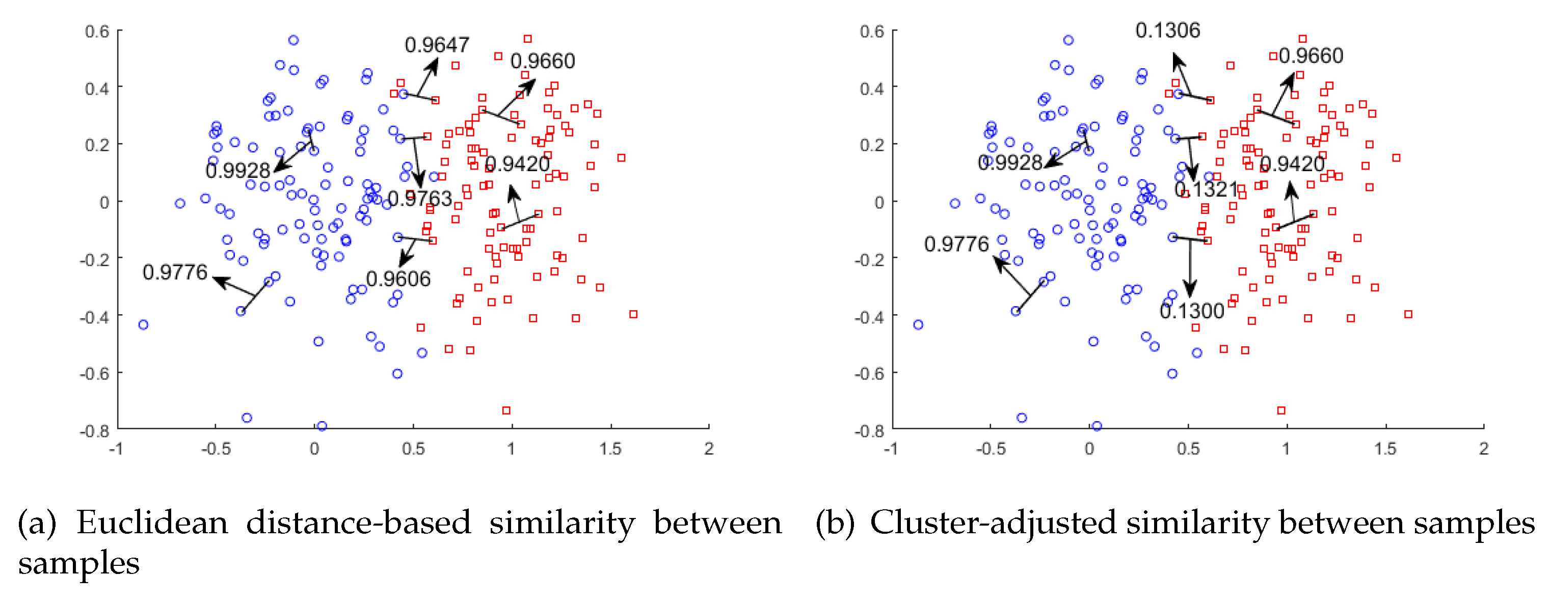
Although these approaches improve the performance of LE, they still have problems when embedding instances close to the decision boundary. For example, as shown in Figure 1a, instances from different clusters close to the decision boundary may be much closer than instances from the same cluster. As a result, they will be placed nearby in the reduced low-dimensional space, which misleads the data distribution and compromises the learning performance.
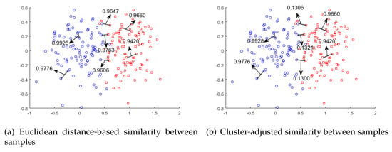
Figure 1.
Comparisons between two types of similarities between samples, shown as (a) and (b). The clustering-adjusted similarity clearly tunes down the Euclidean-based similarity between two instances from different clusters.
To remedy the issue illustrated in Figure 1, we proposed Laplacian Eigenmaps dimensionality reduction based on Clustering-Adjusted Similarity (LE-CAS). LE-CAS applies clustering technique on the original instances to explore the underlying data distribution and global structure of instances. At this stage, we initially intended to use k-means clustering [22] as the method to obtain the decision boundaries. However, as our feature space has large scale and complex structure, the clusters produced by k-means clustering depends largely on the distribution of samples and may not be related to the structure of the boundaries. To solve this kind of problem, we decided to employ an optimization method of k-means clustering called kernel k-means [30]. Kernel k-means maps the data to a higher-dimensional feature space through a nonlinear mapping and performs cluster analysis in the feature space. This method of mapping data to high-dimensional space can highlight the feature differences between sample classes and obtain more accurate clustering results. After that, LE-CAS uses the cluster structure to adjust the similarity between instances based on Gaussian heat kernel. In particular, if pairwise instances belong to different clusters, the similarity between them will be reduced based on the original, otherwise the similarity is unchanged. As shown in Figure 1b, the similarities between pairwise samples from different clusters are reduced, while the similarities between samples from the same cluster remain high. In this way, the global structure information revealed by clustering is embedded into the adjusted similarity, which can better capture the structure between samples. Finally, LE-CAS executes Laplacian Eigenmaps dimensionality reduction based on this clustering-adjusted similarity. Extensive experimental results on UCI datasets from different domains show that LE-CAS significantly outperforms other approaches, which aim to improve LE by different techniques.
The structure of this paper is organized as follows. In Section 2, we give the details of how to adjust similarity between samples and list the procedures of LE-CAS. The preparatory works of the experiment are introduced in Section 3, experimental results and analysis on UCI datasets are presented in Section 4, followed with conclusions and future work in Section 5.
2. Methodology
Suppose be n instances in the d-dimensional space. LE-CAS targets to project into a low-dimensional subspace with new representation with . At the beginning of this section, we would like to introduce the basic idea inside our method called Clustering-Adjusted Similarity (CAS) [31]. In addition, then we will briefly illustrate the proceeding of our LE-CAS.
2.1. Clustering-Adjusted Similarity
The GEDR methods often resort to a typical similarity metric to capture the similarity between samples and structure among them. In this paper, we start with the widely used Gaussian heat kernel as follows:
where is Gaussian hear kernel width. represents the similarity between and , and . can be viewed as a weighted adjacency matrix of a graph, which stores the pairwise similarity between n samples. This way of graph construction is proved to be a simple and effective solution by previous studies [13].
However, for pairs of instances located close to the decision boundary but from different classes, they have a high similarity (see two instances in different clusters but with high similarity 0.9674 in Figure 1a), which mislead them being close in the projected subspace. To mitigate the problem, we aim at reducing the similarity between instances close to decision boundary, which are from different clusters, while remaining the high similarity between samples of the same cluster. To reach that target, we apply CAS as described below.
CAS is based on the idea that samples in the same cluster are similar and those in different clusters should be dissimilar as much as much possible. To explore the clusters of the origin instances, we perform kernel k-means clustering on all instances. Suppose the set of the final clusters is , m is the number of clusters and represents the h-th cluster. , and . The cluster centroids () of the h-th cluster is:
is the number of instances placed into the h-th cluster. Then the similarity between two cluster centroids is similarly defined based on the Gaussian heat kernel as follows:
is the Gaussian heat kernel similarity between and . Obviously, the similarity between two cluster centroids is small when the distance in Euclidian measurement is large.
To facilitate the clustering-based adjustment, we define as follows:
is the label indicator matrix, each row corresponds to an instance and each column for a distinct label. d represents the number of clusters of the whole instances. If instance belong to the h th cluster, , otherwise, .
Finally, the original Gaussian heat kernel similarity data matrix is adjusted into as follows:
From the definition of and , we can find that for two samples (i and j) placed into the same cluster , since , . On the other hand, for two samples from different clusters, shrinks to , since and .
2.2. Laplacian Eigenmap-Based Clustering-Adjusted Similarity
Based on the clustering-adjusted similarity, we present the procedure of LE-CAS as follows, and the influence of our improved method is also shown in Figure 1.
- Carry out kernel k-means clustering on the original dataset , the original data is clustered into classes. During the clustering, we first use an nonlinear mapping function to map the instances from the original space to a higher-dimensional space F, and then clustering in this space.The instances of the original space becomesOn this basis, kernel clustering is to minimize the following criterion function, is the class-mean of i-th cluster.After clustering, we get the following groups:
- Construct a graph with the edge weight between and specified as Equation (1) (, are instances in ). Set up edges between each point and its nearest points via kNN method, is a preset value. This graph will continue to be used in the following steps.
- To determine the weight between points, which is different from typical LE method, the adjusted weight matrix calculated according to Equation (11) before is selected as the final weight matrix of the previous graph. is Gaussian heat kernel width, , represents the cluster centroids of the cluster which and belongs to. , are indicative vectors.
- Construct graph Laplace matrix , is a diagonal matrix with its (i, i)-element equal to the sum of the i th row of
- The objective function of Laplace feature mapping optimization is as follows:and are the representation of instance i, j in the target c-dimensional subspace . The objective function after transform is as follows:Where the constraint function guarantees the optimization problem has solutions.
- Do feature mapping, and calculate the eigenvectors and eigenvalues of . The column vectors of Y that minimize the formula are the eigenvectors corresponding to c minimum non-zero eigenvalues (including multiple roots) of the generalized eigenvalue problem. The smallest c eigenvectors which are correspond to the non-zero eigenvalues are used as the output after dimensionality reduction.
3. Experiment Setup
3.1. Datasets
We employ experiments on ten publicly available UCI datasets to quantitatively evaluate the performance of LE-CAS. The statistics of these datasets are listed in Table 1. These datasets are with different numbers of features and of samples: Msplice represents dataset on molecular biology splice online learning, which is used for multiclass clustering. W1a data set records information from a TV series called W1A. Soccer-sub1 stores the information on players registered in FIFA. Madelon is an artificial dataset, which was part of the NIPS 2003 feature selection challenge. This is a two-class classification problem with continuous input variables. FG-NET is a dataset used for face recognition. ORL contains 400 images of 40 different people, was created by the Olivetti research laboratory in Cambridge, England, between April 1992 and April 1994. Musk describes a set of 102 molecules of which 39 are judged by human experts to be musks and the remaining 63 molecules are judged to be non-musks. CNAE-9 is a data set containing 1080 documents of free text business descriptions of Brazilian companies categorized into a subset of 9 categories cataloged in a table called National Classification of Economic Activities. SECOM is about data from a semi-conductor manufacturing process. DrivFace contains images sequences of subjects while driving in real scenarios. All data sets are available from the UCI Machine Learning Repository (http://archive.ics.uci.edu/ml/index.php).

Table 1.
Statistics of datasets used for experiments.
3.2. Comparing Methods
We compare LE-CAS against four different GDR methods: the original LE [21], GGLE [27], S-LE [28] and SCPLE [29]. The latter three comparing methods try to improve LE from different aspects and have close connection with our work. These comparing methods were introduced in Section 1. We first apply these dimensionality reduction methods to project the high-dimensional samples into a low-dimensional subspace. After that, the widely adopted k-means [22] clustering is applied to cluster the samples projected in the subspace by the respective comparing method.
In the experiments, we specify (or optimize) the input parameters of these comparing methods as the authors suggested in the original papers. As to LE-CAS, is determined by calculating the contour coefficient to obtain a better result of initial clustering. =10 is used to construct kNN graph. The sensitivity of for these kNN graph-based methods (LE [21], GGLE [27], and LE-CAS) and for Gaussian heat kernel function-based methods (GGLE [27], LE-CAS) will be studied later.
3.3. Evaluation Metrics
To evaluate the performance of different dimensionality reduction methods, we adopt four frequently used clustering-effect evaluation index: Fowlkes and Mallows Index (FMI) [32], F-measure [33] and Purity (PU) [34].
For dataset , it is assumed that the cluster obtained through clustering is divided into , and the cluster given by the reference model is divided into . Accordingly, let and respectively represent the cluster marker vectors corresponding to and . We consider the sample pairwise, as defined below: , , , .
set contains sample pairs which belong to the same cluster in are still belong to the same cluster in , set contains sample pairs which belong to the same cluster in are not belong to the same cluster in . set contains sample pairs which not belong to the same cluster in are belong to the same cluster in , set contains sample pairs which not belong to the same cluster in are still not belong to the same cluster in . a, b, c, d represents the number of data pairs in set , , , . Thus,
F-measure is based on precision and recall of clustering results:
Purity represents the number of samples with correct clustering in the total number of samples. represents total number of samples, is the collection of cluster, represents h-th cluster, is the collection of sample, represents i-th sample. Computational formula is shown as below:
4. Results
4.1. Results on Different Datasets
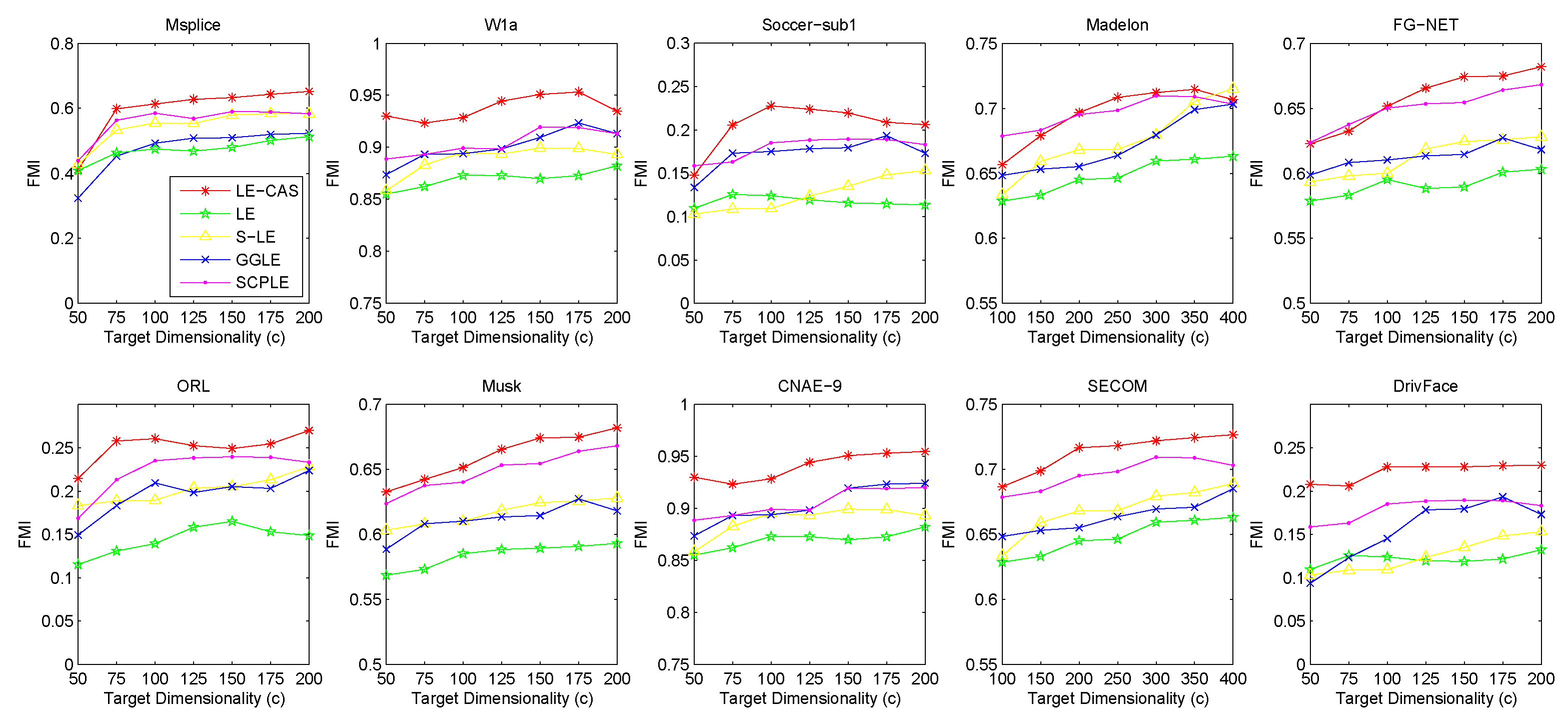
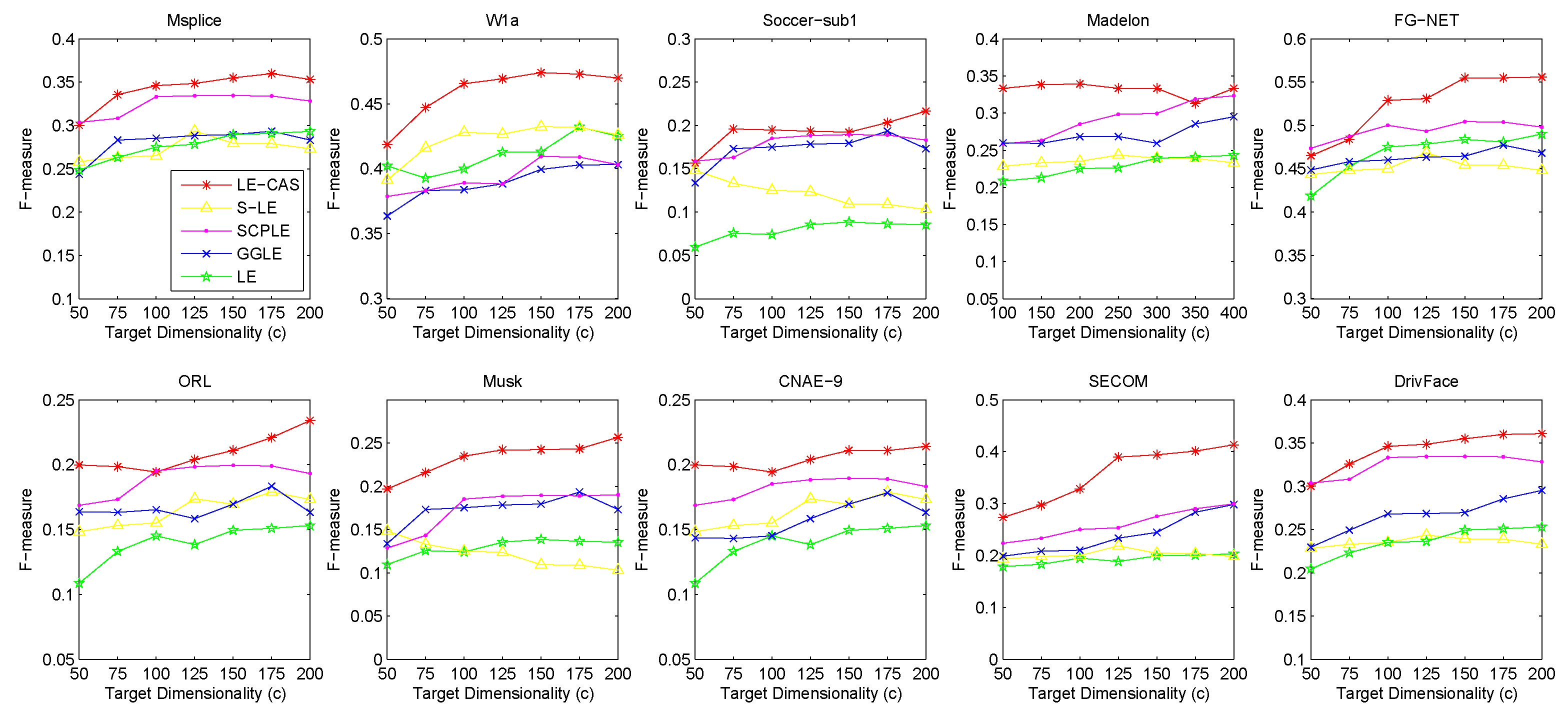
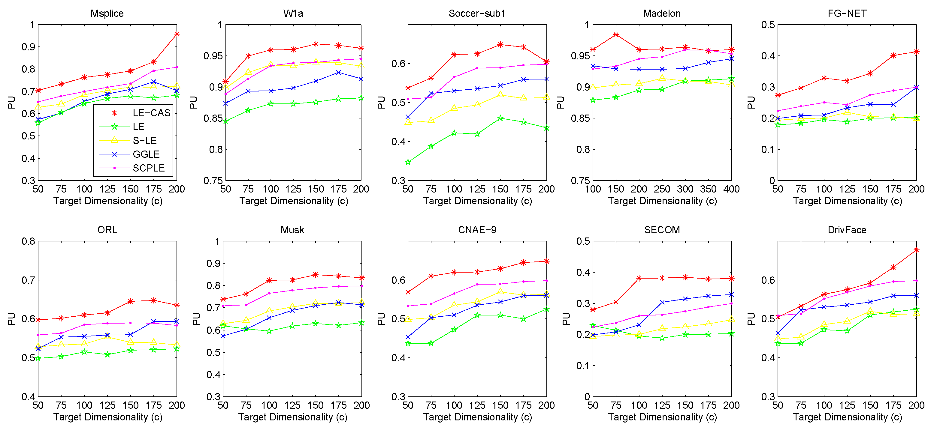
Figure 2 (for FMI’s performance), Figure 3 (for F-measure’s performance) and Figure 4 (for PU’s performance) show the results with respect to different fixed target dimensionality after applying different dimensionality reduction solutions and with the same k-means clustering. To avoid random effects, we repeated the experiment for 30 times and calculated the mean and variance of the results of LE-CAS and comparing methods with respect to four evaluation metrics on respective datasets, which is shown on Table 2.
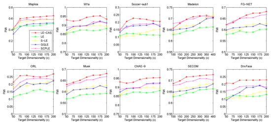
Figure 2.
Results of FMI on ten datasets (Msplice, W1a, Soccer-sub1, Medelon, FG-NET, ORL, Musk, CNAE-9, SECOM, DrivFace) under different target dimensionalities (c).
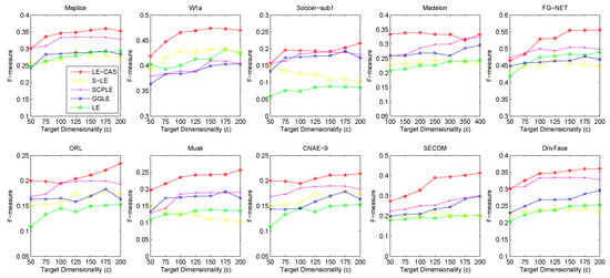
Figure 3.
Results of F-measure on ten datasets (Msplice, W1a, Soccer-sub1, Medelon, FG-NET, ORL, Musk, CNAE-9, SECOM, DrivFace) under different target dimensionalities (c).
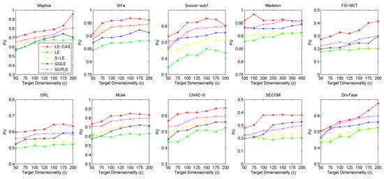
Figure 4.
Results of PU on ten datasets (Msplice, W1a, Soccer-sub1, Medelon, FG-NET, ORL, Musk, CNAE-9, SECOM, DrivFace) under different target dimensionalities (c).

Table 2.
Results (average ± std) of comparing methods on different datasets (Msplice, W1a, Soccer-sub1, Medelon, FG-NET, ORL, Musk, CNAE-9, SECOM, DrivFace). The target dimensionality c is set to 10. The best (or comparable to the best) results are in boldface.
According to the table and figures, we can observe that the performances of all methods increases with the target dimensionality rising and LE-CAS always outperforms other comparing methods across all the evaluation metrics and six datasets. LE-CAS and LE both uses Laplacian Eigenmaps, while LE-CAS achieves better performance on four evaluation indices than that of the LE. That is because LE-CAS changes the similarity calculation method of the instances on the decision boundary, and the adjacent instances are still close enough and the clusters they belong to remain the same after dimensionality reduction. The fact indicates the clustering similarity adjustment (CAS) can improve the performance of GEDR methods.
LE-CAS and GGLE both uses Gaussian kernel function (LE-CAS calculated the similarity between clusters and instances by Gaussian kernel function, GGLE measures similarity between instances via different generalized Gaussian kernel functions), while the performance of GGLE is much lower than that of LE-CAS. This fact shows that CAS used by LE-CAS can better reflect the real relationship between the instances than generalized Gaussian kernel functions used by GGLE.
The performance of LE-CAS is better than that of S-LE and SCPLE, which use the ratio of Euclidean distance to geodesic distance between two instances adjusts the number of nearest neighbors. That is because the clustering-adjusted similarity can more well explore the geometric structure of instances than adaptive adjustment of neighborhood parameters. SCPLE performs better than S-LE, which verifies that SCPLE is an improved method based on S-LE via concerning neighborhood parameter of instances from same or different clusters.
As for stability, LE-CAS performs well, the variance is basically stable and its effect of cluster can maintain good stability in different target dimensions, while the variance of other improved LE methods fluctuates and its effect of cluster has a complex turbulence into different target dimensions at the same time. That is because the similarity without CAS can be easily destroyed by noisy featured.
After detailed observations of the results on different datasets, we found that the FMI results on several datasets are much lower than others (Look at the FMI values on dataset soccer-sub1, ORL, DrivFace). Since FMI is an evaluation index which measures the consistency between the clustering results and the real labels as we mentioned before, there are good reasons to believe that clustering occur in these datasets are not so perfect, which means that the clusters identified by the clustering method we used in LE-CAS (kernel k-means) are not well suitable for the true decision boundaries. Fortunately, even though the clusters we obtained are not so satisfied, the performance of the LE-CAS is still better than the performance of GGLE, S-LE, SCPLE and LE, we can still get relatively good results.
4.2. Parameter Sensitivity Analysis
Because we adopted kernel k-means just as data preprocessing in our approach, so for the determination of value, we make the from 2 to 10, repeat several times kernel k-means on each value (to avoid local optimal solution), and calculate the current average contour coefficient. Finally, the corresponding to the maximum contour coefficient is selected as the final number of clusters.
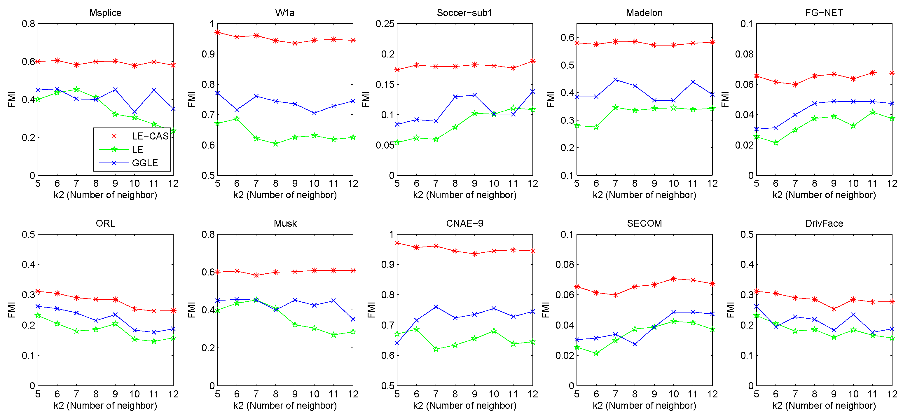
LE-CAS, LE, and GGLE make use of a kNN graph to set up the adjacency matrix and the weights between samples, and hence for graph-based dimensionality reduction. To study the sensitivity of these methods to the input value of , we increase from 5 to 12, and report the FMI values of these algorithms under each input value of (number of neighbors) in Figure 5.
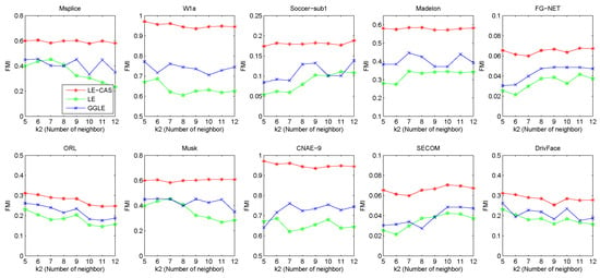
Figure 5.
Results (FMI) vs. on ten datasets (Msplice, W1a, Soccer-sub1, Medelon, FG-NET, ORL, Musk, CNAE-9, SECOM, DrivFace).
From this figure, we can observe that no matter how the value changes, the results of LE-CAS on these datasets are better than those of another two comparing algorithms. Fluctuations mainly happen in LE and GGLE, while LE-CAS gets a relatively smooth curve. GGLE adopts the kNN graph constructed in the original high-dimensional space to explore the local geometric structure of samples. It uses the nearest neighbors of a sample to seek the linear relationships between nearest neighbors. Therefore, it still focuses on the local manifold, and is sensitive to . As increase, the linear relationship between them becomes increasingly complicated, which causes the increase of error rate. LE and LE-CAS also adopt the kNN graph, LE-CAS additionally uses the global cluster structure of samples to adjust the similarity between neighborhood samples. The performance margin between LE-CAS and LE, and the better stability of LE-CAS proves the effectiveness of clustering-adjusted similarity. From these results, we can conclude LE-CAS is robust to noise and can work well under a wide range of input values of .
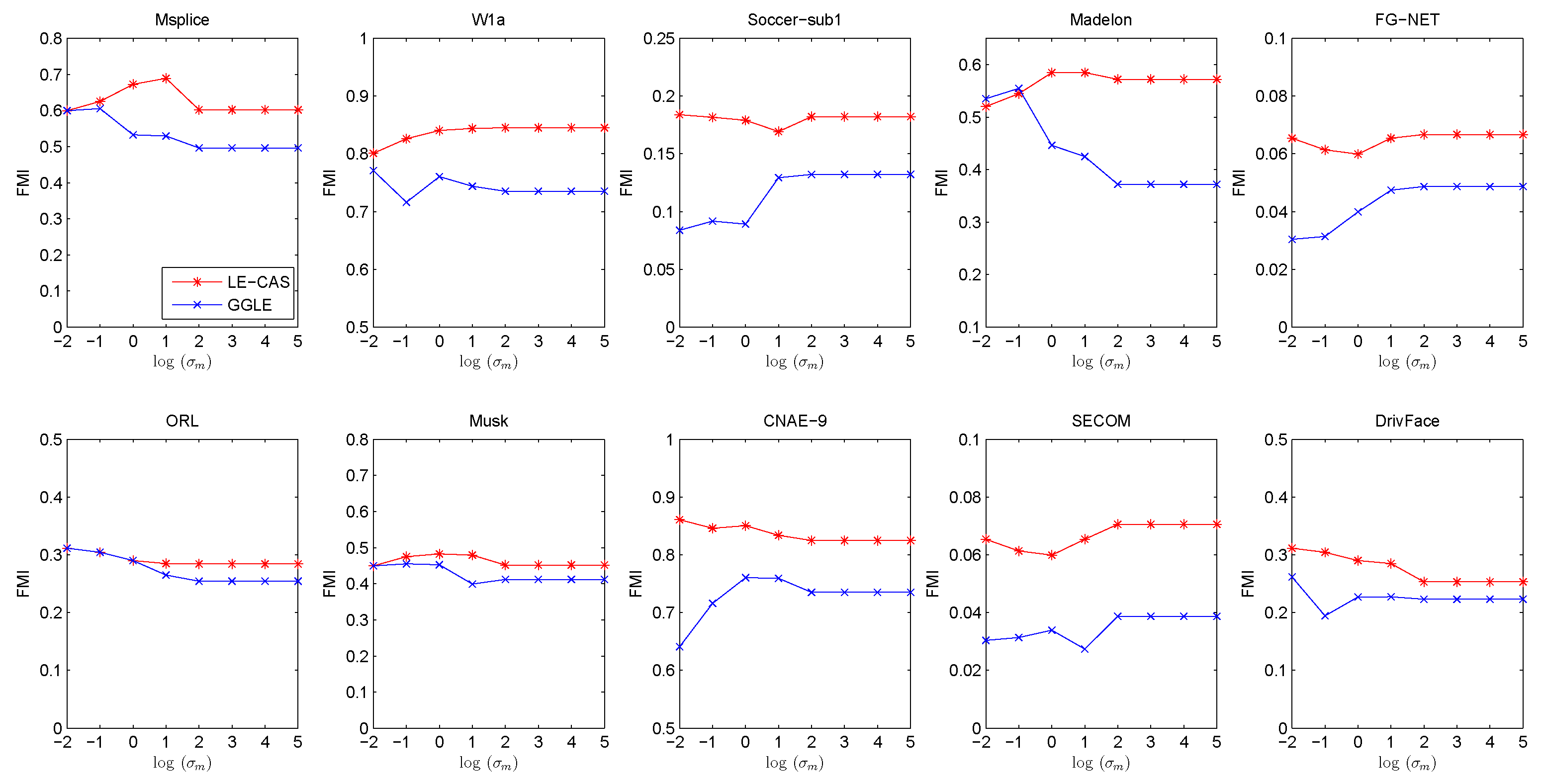
Both LE-CAS and GGLE specify edge weight by Gaussian heat kernel function. From Equation (11), we can see that they both rely on a suitable Gaussian heat kernel width . should not be too small or too large. If is too small, the similarity in Equation (11) will be close to 0, On the other hand, should not be too big. If is too big, the similarity in Equation (11) will be close to 1. In our previous experiments, we set as the mean of square Euclidean distance between all training instances for both LE-CAS and GGLE. To investigate the sensitivity of on LE-CAS and GGLE, we conduct experiments to investigate the influence of . In the following experiments, we increase from to for LE-CAS and GGLE. Other parameter settings are kept the same with previous experiments. Similarly, we run 30 independent experiments for each fixed and report the FMI under each in Figure 6.
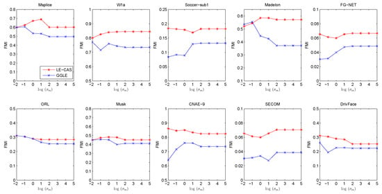
Figure 6.
Results (FMI) vs. on ten datasets (Msplice, W1a, Soccer-sub1, Medelon, FG-NET, ORL, Musk, CNAE-9, SECOM, DrivFace).
From Figure 6, we can find that LE-CAS outperforms LGC in a wide range of . Both GGLE and LE-CAS depend on a suitable . The performance of two methods reaches relatively stable with the increase in . The FMI of LE-CAS is similar to GGLE when is too small. This is because if is too small, the clustering-adjusted similarity is similar to the original Gaussian heat kernel similarity. The performance of both LE-CAS and GGLE becomes relatively stable when ≥ 100 in our experiments, and LE-CAS performs significantly better than GGLE. The reason is that the clustering-adjusted similarity has its effect. From the above results, we can conclude that LE-CAS effectively improves the performance of GEDR methods and makes stable performance in a wide range of .
4.3. Robustness Analysis
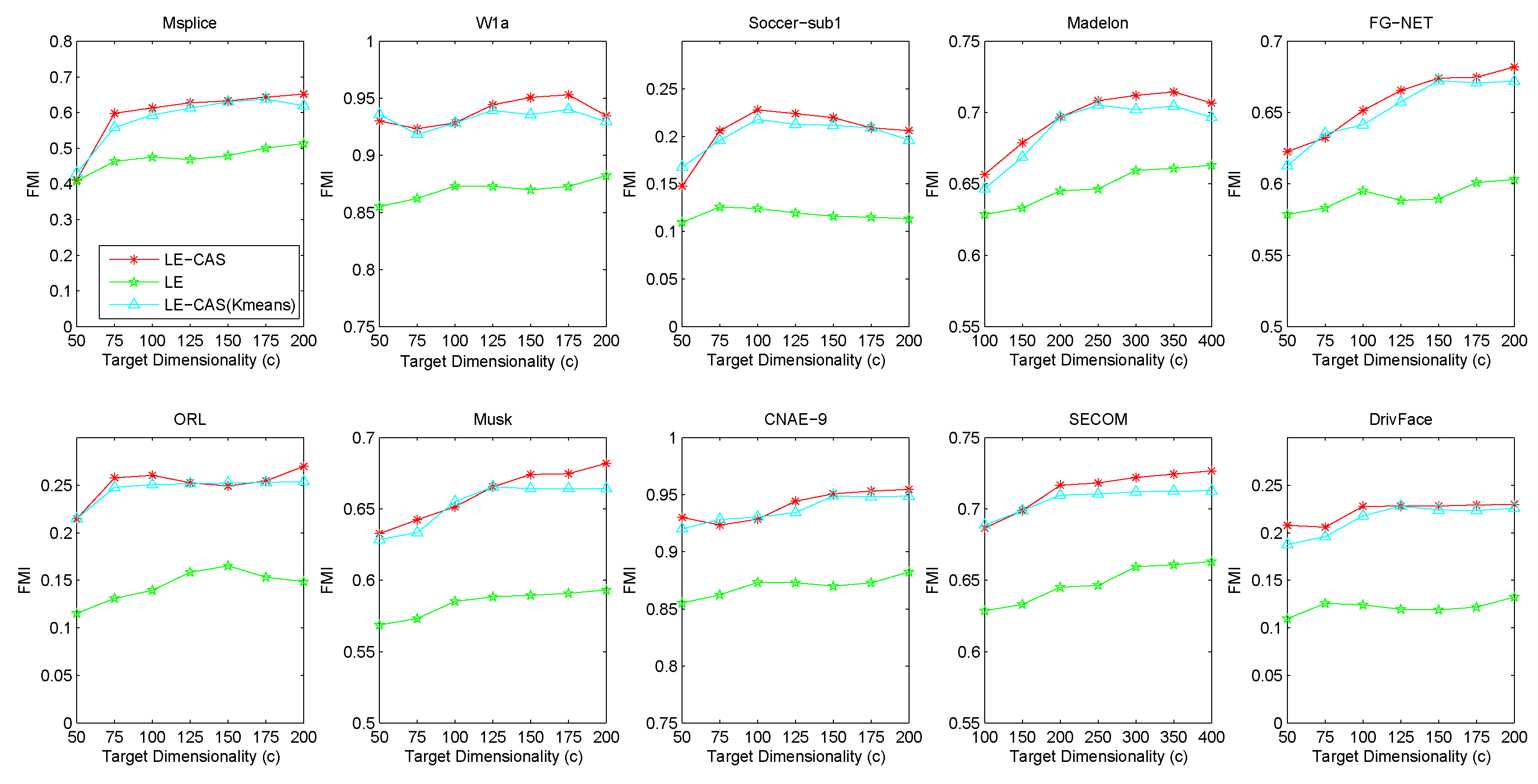
Since our method combines clustering with dimensionality reduction, the performance of LE-CAS seems heavily depends on whether the clustering method used in previous steps. To clarify the robustness of our method, we employed two different clustering methods, k-means and kernel k-means, as the initial clustering method in the course of LE-CAS. The performance of these methods are shown as Figure 7.
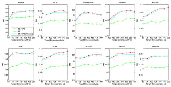
Figure 7.
Results of FMI on ten datasets (Msplice, W1a, Soccer-sub1, Medelon, FG-NET, ORL, Musk, CNAE-9, SECOM, DrivFace) under different target dimensionalities (c).
From Figure 7, we can illustrate that the performances of two clustering methods are merely close to each other on ten datasets and each method performs better than LE method, which indicates that the performance of our LE-CAS cannot be influenced much by the clustering method used in initial steps.
5. Conclusions
In this paper, we introduced the Laplacian Eigenmaps dimensionality reduction based on Clustering-Adjusted Similarity(LE-CAS), which leverages local manifold structure and global cluster structures to adjust the similarity between neighborhood samples. In particular, the adjusted similarity can reduce the similarity between pairwise samples from different clusters while maintain the similarity between samples of the same cluster. Experimental results on public benchmark datasets show that that the clustering-adjusted similarity improve the performance of classical LE and outperforms other related competitive solutions.
In our future work, we want to explore other principle ways to refine the similarity between instances and further improve the performance of GEDR methods. In addition, we will pay more attention to weakly supervised graph-based dimensionality reduction. Otherwise, for problems happened near the decision boundary, fuzzy set theory may also can help. We are willing to compare our method to fuzzy set theory in the future.
Author Contributions
Conceptualization, J.W.; Investigation, H.Z.; Methodology, H.Z. and J.W.; Supervision, J.W.; Validation, H.Z.; Writing—original draft, H.Z.; Writing—review & editing, J.W.
Funding
This research received no external funding.
Acknowledgments
This work is supported by Natural Science Foundation of China (61873214), Fundamental Research Funds for the Central Universities (XDJK2019B024).
Conflicts of Interest
The authors declare no conflict of interest. The founding sponsors had no role in the design of the study; in the collection, analyses, or interpretation of data; in the writing of the manuscript, and in the decision to publish the results.
References
- Song, M.; Yang, H.; Siadat, S.H.; Pechenizkiy, M. A comparative study of dimensionality reduction techniques to enhance trace clustering performances. Expert Syst. Appl. 2013, 40, 3722–3737. [Google Scholar] [CrossRef]
- Fan, M.; Gu, N.; Hong, Q.; Bo, Z. Dimensionality reduction: An interpretation from manifold regularization perspective. Inf. Sci. 2014, 277, 694–714. [Google Scholar] [CrossRef]
- Vlachos, M.; Domeniconi, C.; Gunopulos, D.; Kollios, G.; Koudas, N. Non-linear dimensionality reduction techniques for classification and visualization. In Proceedings of the eighth ACM SIGKDD International Conference on Knowledge Discovery & Data Mining, Edmonton, AB, Canada, 23–26 July 2002; pp. 645–651. [Google Scholar]
- Tao, M.; Yuan, X. Recovering Low-Rank and Sparse Components of Matrices from Incomplete and Noisy Observations. SIAM J. Optim. 2011, 21, 57–81. [Google Scholar] [CrossRef]
- Shi, L.; He, P.; Liu, E. An incremental nonlinear dimensionality reduction algorithm based on ISOMAP. In Proceedings of the Australian Joint Conference on Advances in Artificial Intelligence, Sydney, Australia, 5–9 December 2005; pp. 892–895. [Google Scholar]
- Massini, G.; Terzi, S. A new method of Multi Dimensional Scaling. Fuzzy Information Processing Society; IEEE: Toronto, ON, Canada, 2010; ISBN 978-1-4244-7859-0. [Google Scholar]
- Vel, O.D.; Li, S.; Coomans, D. Non-Linear Dimensionality Reduction: A Comparative Performance Analysis. In Learning from Data; Springer: Berlin, Germany, 1996; pp. 323–331. [Google Scholar]
- Leinonen, T. Principal Component Analysis and Factor Analysis, 2nd ed.; Springer: New York, NY, USA, 2004; ISBN 978-0-387-95442-4. [Google Scholar]
- Roweis, S.T.; Saul, L.K. Nonlinear Dimensionality Reduction by Locally Linear Embedding. Science 2000, 290, 2323–2326. [Google Scholar] [CrossRef]
- Belkin, M.; Niyogi, P. Laplacian eigenmaps and spectral techniques for embedding and clustering. Adv. Neural Inf. Process. Syst. 2001, 14, 585–591. [Google Scholar]
- Dornaika, F.; Assoum, A. Enhanced and parameterless Locality Preserving Projections for face recognition. Neurocomputing 2013, 99, 448–457. [Google Scholar] [CrossRef]
- Qiang, Y.; Rong, W.; Bing, N.L.; Yang, X.; Yao, M. Robust Locality Preserving Projections With Cosine-Based Dissimilarity for Linear Dimensionality Reduction. IEEE Access 2017, 5, 2676–2684. [Google Scholar]
- He, X. Locality Preserving Projections. Ph.D. Thesis, University of Chicago, Chicago, IL, USA, 2005. [Google Scholar]
- Yu, G.; Hong, P.; Jia, W.; Ma, Q. Enhanced locality preserving projections using robust path based similarity. Neurocomputing 2011, 74, 598–605. [Google Scholar] [CrossRef]
- Deng, C.; He, X.; Han, J. Semi-supervised Discriminant Analysis. In Proceedings of the IEEE 11th International Conference on Computer Vision, Rio de Janeiro, Brazil, 14–21 October 2007; pp. 1–8. [Google Scholar]
- Bunte, K.; Schneider, P.; Hammer, B.; Schleif, F.M.; Villmann, T.; Biehl, M. Limited Rank Matrix Learning, discriminative dimension reduction and visualization. Neural Netw. 2012, 26, 159–173. [Google Scholar] [CrossRef]
- Song, Y.; Nie, F.; Zhang, C.; Xiang, S. A unified framework for semi-supervised dimensionality reduction. Pattern Recognit. 2008, 41, 2789–2799. [Google Scholar] [CrossRef]
- Yu, G.X.; Peng, H.; Wei, J.; Ma, Q.L. Mixture graph based semi-supervised dimensionality reduction. Pattern Recognit. Image Anal. 2010, 20, 536–541. [Google Scholar] [CrossRef]
- Yan, S.; Xu, D.; Zhang, B.; Zhang, H.J.; Yang, Q.; Lin, S. Graph embedding and extensions: A general framework for dimensionality reduction. IEEE Trans. Pattern Anal. Mach. Intell. 2007, 29, 40–51. [Google Scholar] [CrossRef] [PubMed]
- Effrosyni, K.; Yousef, S. Orthogonal neighborhood preserving projections: A projection-based dimensionality reduction technique. IEEE Trans. Pattern Anal. Mach. Intell. 2007, 29, 2143–2156. [Google Scholar]
- Belkin, M.; Niyogi, P. Laplacian Eigenmaps for Dimensionality Reduction and Data Representation. Neural Comput. 2003, 15, 1373–1396. [Google Scholar] [CrossRef]
- Trad, M.R.; Joly, A.; Boujemaa, N. Large Scale KNN-Graph Approximation. In Proceedings of the 2012 IEEE 12th International Conference on Data Mining Workshops, Brussels, Belgium, 10 December 2012; pp. 439–448. [Google Scholar]
- Tenenbaum, J.B.; De Silva, V.; Langford, J.C. A global geometric framework for nonlinear dimensionality reduction. Science 2000, 290, 2319–2323. [Google Scholar] [CrossRef]
- Weinberger, K.Q.; Saul, L.K. An introduction to nonlinear dimensionality reduction by maximum variance unfolding. AAAI 2006, 6, 1683–1686. [Google Scholar]
- Weinberger, K.Q.; Saul, L.K. Unsupervised learning of image manifolds by semidefinite programming. Int. J. Comput. Vis. 2006, 70, 77–90. [Google Scholar] [CrossRef]
- Parsons, L.; Haque, E.; Liu, H. Subspace clustering for high dimensional data: A review. ACM Sigkdd Explor. Newsl. 2004, 6, 90–105. [Google Scholar] [CrossRef]
- Zeng, X.; Luo, S.; Wang, J.; Zhao, J. Geodesic distance-based generalized Gaussian Laplacian Eigenmap. J. Softw. 2009, 20, 815–824. [Google Scholar]
- Raducanu, B.; Dornaika, F. A supervised non-linear dimensionality reduction approach for manifold learning. Pattern Recognit. 2012, 45, 2432–2444. [Google Scholar] [CrossRef]
- Ning, W.; Liu, J.; Deng, T. A supervised class-preserving Laplacian eigenmaps for dimensionality reduction. In Proceedings of the International Conference on Natural Computation, Fuzzy Systems and Knowledge Discovery, Changsha, China, 13–15 August 2016; pp. 383–389. [Google Scholar]
- Dhillon, I.S.; Guan, Y.; Kulis, B. Kernel k-means, Spectral Clustering and Normalized Cuts. In Proceedings of the Tenth ACM SIGKDD International Conference on Knowledge Discovery and Data Mining, Seattle, WA, USA, 22–25 August 2004; pp. 551–556. [Google Scholar]
- Chen, X.; Lu, C.; Tan, Q.; Yu, G. Semi-supervised classification based on clustering adjusted similarity. Int. J. Comput. Appl. 2017, 39, 210–219. [Google Scholar] [CrossRef]
- Nemec, A.F.L.; Brinkhurst, R.O.B. The Fowlkes Mallows statistic and the comparison of two independently determined dendrograms. Can. J. Fish. Aquat. Sci. 1988, 45, 971–975. [Google Scholar] [CrossRef]
- Liu, Z.; Tan, M.; Jiang, F. Regularized F-measure maximization for feature selection and classification. BioMed Res. Int. 2009, 2009, 617946. [Google Scholar] [CrossRef] [PubMed]
- Aliguliyev, R.M. Performance evaluation of density-based clustering methods. Inf. Sci. 2009, 179, 3583–3602. [Google Scholar] [CrossRef]
© 2019 by the authors. Licensee MDPI, Basel, Switzerland. This article is an open access article distributed under the terms and conditions of the Creative Commons Attribution (CC BY) license (http://creativecommons.org/licenses/by/4.0/).

