A Distributed Execution Pipeline for Clustering Trajectories Based on a Fuzzy Similarity Relation

Abstract

The proliferation of indoor and outdoor tracking devices has led to a vast amount of spatial data. Each object can be described by several trajectories that, once analysed, can yield to significant knowledge. In particular, pattern analysis by clustering generic trajectories can give insight into objects sharing the same patterns. Still, sequential clustering approaches fail to handle large volumes of data. Hence, the necessity of distributed systems to be able to infer knowledge in a trivial time interval. In this paper, we detail an efficient, scalable and distributed execution pipeline for clustering raw trajectories. The clustering is achieved via a fuzzy similarity relation obtained by the transitive closure of a proximity relation. Moreover, the pipeline is integrated in Spark, implemented in Scala and leverages the Core and Graphx libraries making use of Resilient Distributed Datasets (RDD) and graph processing. Furthermore, a new simple, but very efficient, partitioning logic has been deployed in Spark and integrated into the execution process. The objective behind this logic is to equally distribute the load among all executors by considering the complexity of the data. In particular, resolving the load balancing issue has reduced the conventional execution time in an important manner. Evaluation and performance of the whole distributed process has been analysed by handling the Geolife project’s GPS trajectory dataset.

1. Introduction

In our time, billions of events are generated by location-aware devices in a matter of seconds. The extracted events’ knowledge can be leveraged to increase economic gain, reinforce security and support decision making. In particular, the pattern analysis of the moving object trajectories can make it possible to understand or predict behaviour. Hence, cluster analysis has been quite indispensable. Still, the real-time, fuzzy, heavy nature of events has been a burden for conventional clustering approaches. Consequently, researchers have taken interest in fields like big data, online clustering and fuzzy logic.

Big data technologies often refer to notions like concurrency, distribution, parallelism and stream processing. Mainly, deployed in a cluster environment where the memory and storage can be shared by the cluster’s nodes. The nodes can be located in the same location or distributed among regions with a possible peer-to-peer or master–slave connection strategy. High Availability, mass storage, mass computing and fault tolerance are primarily featured by big data ecosystems. In this study, we take interest in leveraging the functionalities of Spark (https://spark.apache.org/) into clustering trajectories. The choice is supported by the fast computing nature of spark explained by its use of the Random Access Memory (RAM). In particular, we analyse the Geolife project’s GPS trajectory dataset [1,2,3]. The dataset is stored in HDFS and an entire pipeline for reading, manipulating and defining clusters is being detailed in this paper. Clustering is done by computing the max–min transitive closure of a fuzzy proximity relation. Several trajectory similarity indices exist on the literature [4] and reasoning about which one is more accurate than the others is out of the scope of this paper. Consequently, for simplicity we consider the Longest Common Subsequence’s (LCSS) length [5]. In the process, we have included the max–min, max–delta and max–product transitivity. An option of both the smart [6] and semi-naive [7] algorithms is deployed for computing the transitive closure. The system is implemented in Scala; hence, futures, traits, objects and higher-order functions are integrated to enrich the system’s model. The pipeline’s activity diagrams, system’s class diagrams and different algorithms are detailed. Furthermore, we have encountered an issue related to unbalanced workloads; thus, we propose a new partitioning logic that considers the complexity of data and equally partitions it across the executors. By resolving the load balancing issue, the computation time was significantly reduced. After defining the clusters, we persist the results in a MongoDB (https://www.mongodb.com/) collection by leveraging the reactive mongodb driver (http://reactivemongo.org/) known for its asynchronous nature. This final step can be extended to infer knowledge and analysed for understanding Spark’s behaviour in the asynchronous boundaries. To the best of our knowledge, this is the first research giving a detailed implementation of the raw trajectories clustering process in Spark by leveraging a fuzzy similarity relation, analysing the performance of repartitioning tasks and providing a new partitioning strategy for handling trajectory data skewness and empirical proof of its efficiency.

The rest of this paper involves three sections: Section 2 discusses the existing literature; Section 3 yields a background over fuzzy logic, fuzzy relations, LCSS problem and the trasitive closure; Section 4 provides the different algorithms, class and activity diagrams; Section 5 provides the evaluation of the different partitioning stages; Section 6 concludes our paper and highlights future work.

2. Literature

Since Zadeh initiated fuzzy logic [8], researchers have taken interest in defining fuzzy clusters, which reflect more the fuzzy nature of features, instead of crisp ones. Consequently, fuzzy clustering approaches have emerged. Research on fuzzy clustering can be categorised into approaches leveraging an objective function (fuzzy c-means) and approaches manipulating a proximity relation. The last ones can be further classified into approaches handling directly the proximity relation and approaches proposing techniques to convert the proximity relation into a similarity relation then apply a specific clustering technique to get the different partition trees [9].

Research on directed approaches include [10]. The authors proposed a new approach based on the entropy measure, which lies in $\left[0,1\right]$. The main idea is that this measure between two nodes equals 0 if they are respectively very close or very far from each other and 1 if they get close to the average distance between all nodes. The entropies are measured from a proximity relation and cluster centres defined by the lowest entropies. Boulmakoul et al. [11] defined a quadratic time complexity algorithm for defining clusters from a proximity relation. The authors define a cluster as a maximum weighted clique of nodes. The weights refer to the different similarities. The obtained clusters are both compact and well separated. Both the supra works define a cluster node as a node similar to all the other nodes in the same cluster. In contrast, Kondruk [12] defined an approach based on cluster centres. Each cluster node is similar to the centre and the centres are updated at each iteration. Different algorithms exist in the literature to identify the transitive closure. The most known ones are the smart [6] and semi-naive [7] algorithm. They are leveraged to extract a similarity relation leading to extended clusters. Tamura et al. [13] introduced the max–min transitivity that yields a similarity relation having equivalence relations as a resolution form. Each equivalence relation leads to non-overlapping partition trees. Yang et al. [14] defined max–prod and max–Δ as an extension of the previous work. However, the resulting relation can lead to overlapping partitions. Hence, the necessity for specific algorithms to extract non-overlapping clusters based on a specific cluster definition. Also, the directed approaches can handle these max–t transitive relations to extract non-overlapping clusters. Liang et al. [15] identified clusters by considering a metric of trapezoidal numbers and leveraging the max–min transitivity.

In the scope of the latter approaches, relatively few works have been conducted into evaluating the performance of computing the transitive closure in a distributed environment. In particular, studies [16,17] have proposed new fragmentation techniques for computing the transitive closure in a parallel manner. Gribkoff [18] evaluated the smart and semi-naive algorithm in Hadoop map/reduce environment. Although Spark outperforms Hadoop in processing, none of the previous works have evaluated the transitive closure in its environment. An integration in Spark was only given in [19,20]. Initially, we extended the approach of [11] by leveraging Spark into clustering spatial trajectories. Still, our proposition could not fully distribute the clustering process. Moreover, we have not considered the transitive closure and we did not give a detailed implementation of the distributed proximity relation construction process. In the latter, we applied the max–min transitivity over a proximity relation referring to the similarities between cyber-criminals in Twitter. Unfortunately, we did not evaluate the performance nor have we considered spatial data. Decidedly, the literature includes several works related to trajectory clustering [21] and its applications on resolving real world problems [22]. Still, to the best of our knowledge, this is the first work discussing the exploit of the transitive closure on a fuzzy similarity relation to extract clusters of raw trajectories by using Spark.

3. Background

Definition 1.

Let A be a lexical attribute (warm). The fuzzy set characterising this attribute is denoted $A=\{\langle x,{\mu }_A\left(x\right)\rangle \mid x\in X,{\mu }_A\in [0,1]\}$. The ${\mu }_A$ defines the degree of membership of a lexical variable to the set A. Thus, each element of the universe of discourse $X=\{x_1,x_2\dots ,x_n\}$ can be attributed to several sets with a varying membership degree [23].

Definition 2.

A couple of crisp sets’ elements can be related to each other via a relation. The relation is binary and can be formulated as $R=\{\langle (x,y),{\mu }_R(x,y)\rangle \mid x\in X,y\in Y\}$. In case the relation is crisp the strength of the relationship ${\mu }_R:(X,Y)$ equals 0 or 1. In contrast, a binary fuzzy relation has its membership degrees in $\left[0,1\right]$. In our study, we consider the latter relation.

R has the resolution form $R=\bigcup _{\alpha }\alpha R_{\alpha }$ with $\alpha \in \left[0,1\right]$. $R_{\alpha }$ is a crisp relation with

$${\mu }_{R_{\alpha }}(x,y)=\{\begin{array}{c}1,if{\mu }_R(x,y)\ge \alpha \hfill \\ 0,otherwise\hfill \end{array}$$

R can be denoted a proximity relation if it is both reflexive and symmetric. In particular:

• (Reflexivity): $\forall x\mid X,{\mu }_R(x,x)=1$;
• (Symmetry): $\forall x,y\mid X\times Y,{\mu }_R(x,y)={\mu }_R(y,x)$;

Additionally, if R respects transitivity, it can be refered to as a fuzzy similarity relation. Transitivity is defined as ${\mu }_R(x,z)\ge max\left(T({\mu }_R(x,y),{\mu }_R(y,z))\right)$. T is a t-norm defining the nature of the transitivity; several norms of this kind exist including:

• (max–min transitivity): $T({\mu }_1,{\mu }_2)=min({\mu }_1,{\mu }_2)$;
• (max–Δ transitivity): $T({\mu }_1,{\mu }_2)=max(0,{\mu }_1+{\mu }_2-1)$;
• (max–prod transitivity): $T({\mu }_1,{\mu }_2)={\mu }_1•{\mu }_2$.

Moreover, ${\mathcal{R}}_{\wedge }\subseteq {\mathcal{R}}_{•}\subseteq {\mathcal{R}}_{△}$ with ${\mathcal{R}}_{\wedge },{\mathcal{R}}_{•},{\mathcal{R}}_{△}$ respectively form the set of max–min, max–prod and max–△ transitive relations [24]. In particular, the max–min transitivity yields a fuzzy similarity relation that characterizes each crisp relation in the resolution form as an equivalence relation. Different partition trees can be obtained for each α-level from these equivalence relations [14].

Definition 3.

The fuzzy similarity relation R can be extracted by achieving a series of compositions. A composition has the form $R\circ R=\underset{y}{\max }(\underset{x,z}{T}(R(x,y),R(y,z))$. In our paper, we deploy both the semi-naive and smart algorithm for computing the transitive closure (please see the Section 4.1 for a precise implementation).

Definition 4.

Trajectories can be mainly considered as a temporally ordered sequence and not forcibly related to space in this case they are considered metaphorical. Metaphorical trajectories describe the variations of an attribute over time. Decidedly in the case of an attribute a, $T{r}_a=\{(a_0,t_0),\dots ,(a_n,t_n)\}$ with $t_i$ as a timestamp. Another representation considers the variations of an attribute over abstract spatial regions instead of spatial coordinates, e.g., cities and countries. This representation is referred to as naïve and $T{r}_a=\{(a_0,t_0,C_0),\dots ,(a_n,t_n,C_n)\}$ with $C_i$ the country or region code. In contrast, raw trajectories consider spatial coordinates and describe the spatio-temporal profile of a moving object. Each trajectory has the form $T{r}_{(objec{t}_{id},trajector{y}_{id})}=\{(lon{g}_0,la{t}_0,t_0)\dots (lon{g}_n,la{t}_n,t_n)\}$ with $la{t}_i$ and $lon{g}_i$ respectively denoting the latitude and longitude degrees [25]. In our study, we handle the raw trajectories of the Geolife project’s GPS trajectory dataset [1,2,3].

Definition 5.

Let $T{r}_1$ and $T{r}_2$ be two trajectories, $T{r}_2$ is a subsequence of $T{r}_1$ if all the points in $T{r}_2$ match the points in $T{r}_1$ in an ordered manner with gaps support. The match can reflect respected properties constraints. The longest common subsequence (LCSS) problem can be leveraged to identify similar trajectories. Mainly the LCSS between two trajectories is defined as:

$$LCSS(T{r}_1,T{r}_2)=\{\begin{array}{c}0,if T{r}_1.size=T{r}_2.size\hfill \\ 1+LCSS(T{r}_1.tail, T{r}_2.tail), if the constraints are respected\hfill \\ max(LCSS(T{r}_1.tail, T{r}_2), LCSS(T{r}_1, T{r}_2.tail)), otherwise\hfill \end{array}$$

Different alignments between the two sequences are tested to get the length of the LCSS. [5] identified two points as similar if they respect both a time and distance threshold. Furthermore, they defined the similarity as $S(T{r}_1,T{r}_2)=\frac{LCSS(T{r}_1,T{r}_2)}{max(T{r}_1.size,T{r}_2.size)}$. Aiming to get high similarities, we weaken this constraint into considering either the time or distance. Note that the distance constraint is in meters and the points are defined by their degrees. Hence, we construct from this distance constraint two thresholds [26]:

$$\{\begin{array}{c}l\Delta lat\_th=(distance\_th/earth\_radius)inradians\hfill \\ \Delta long\_th=\mid distance\_th/(r\ast cos(\Delta lat\_th\left)\right)\mid .\hfill \end{array}$$

The points coordinates are converted into radians and their latitude and longitude differences are compared with the supra thresholds.

The recursive nature of the LCSS problem is exponential. An alternative based on memorization has been proposed to resolve the problem in quadratic time and space. Other heuristics have been proposed to give an approximated solution in less time. Still, we stick to the exact approach of [27] which resolves the problem in quadratic time and linear space. The algorithm is described in Algorithm 1. Note that the algorithms in this paper are written in a pseudocode related to the Scala language because the formal way will not be sufficient to express all the functional features.

Algorithm 1: LCSS linear space algorithm.

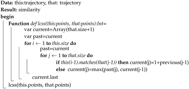4. Materials and Methods

The project is implemented in Scala, aiming to extract clusters from massive trajectory logs stored in HDFS and persist them in MongoDB. Spark is leveraged to conduct the work in a distributed manner. RDD distributed across the memory and disk are being created and the work’s stages are being achieved in parallel by distributing tasks across worker nodes. In particular, the system must provide the possibility to employ either the smart or semi-naive algorithm for computing the transitive closure; the choice of applying either the max–min, max–delta and max–product t-norms for transitivity. Moreover, the max–delta and max–product t-norms need a specific kind of handler.

Theorem 1.

Let $x\in [\alpha ,1]$ and $y\in [\alpha ,1]$ with $\alpha \in [0,1]$. The product $x•y$ is only in $[{\alpha }^2,1]$ but not forcibly in $[\alpha ,1]$.

Proof of Theorem 1.

Let us put $\alpha =1/2$ then $1/4\le x•y\le 1$. For $x•y$ to be in $[\alpha ,1]$, ${\alpha }^2\ge \alpha$ must be true. But, in our case $1/2\ge 1/4$. Hence, by contradiction $x•y\notin [\alpha ,1]$ only in $[{\alpha }^2,1]$. □

Theorem 2.

By considering the same supposition as the Theorem 1. The preposition $x+y-1\ge \alpha$ is not necessarily true, and it holds only if $\alpha =1$.

Proof of Theorem 2.

Let us suppose that $x=y=\alpha$. This is equivalent to $x+y-1=2\alpha -1$. Hence, if $x+y-1\ge \alpha$, then $2\alpha -1\ge \alpha$. The last statement is equivalent to $\alpha \ge 1$, and this holds only if $\alpha =1$ because by our supposition $\alpha \le 1$. Consequently for $\alpha \in [0,1]$, $x+y-1\ge \alpha$ is not always true. □

These two theorems proof that at each step of computing the t-norms, we must filter the norms inferior to the chosen $\alpha$-level. To provide all these possibilities, we present the Figure 1 and Figure 2 explained in the next subsection.

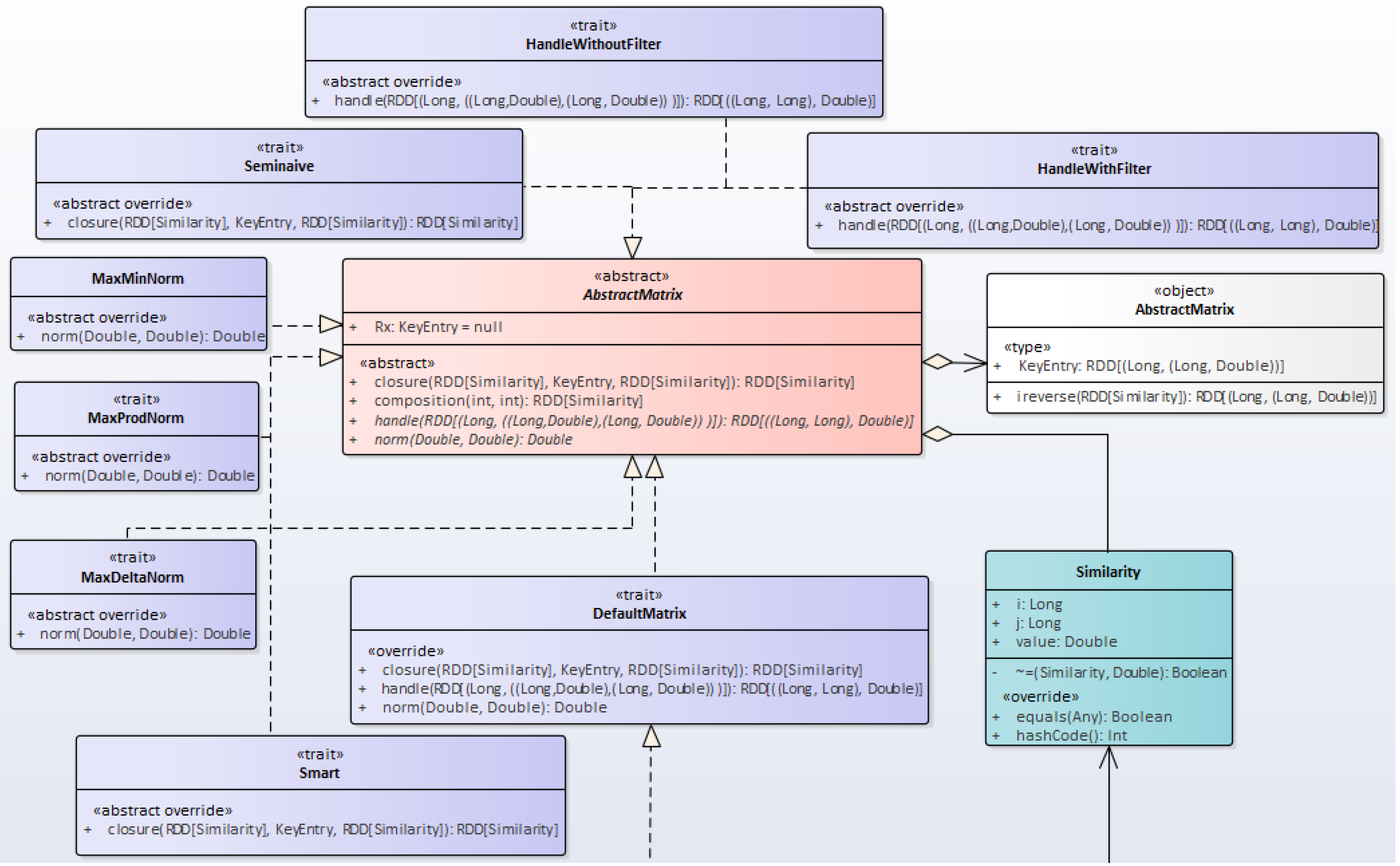
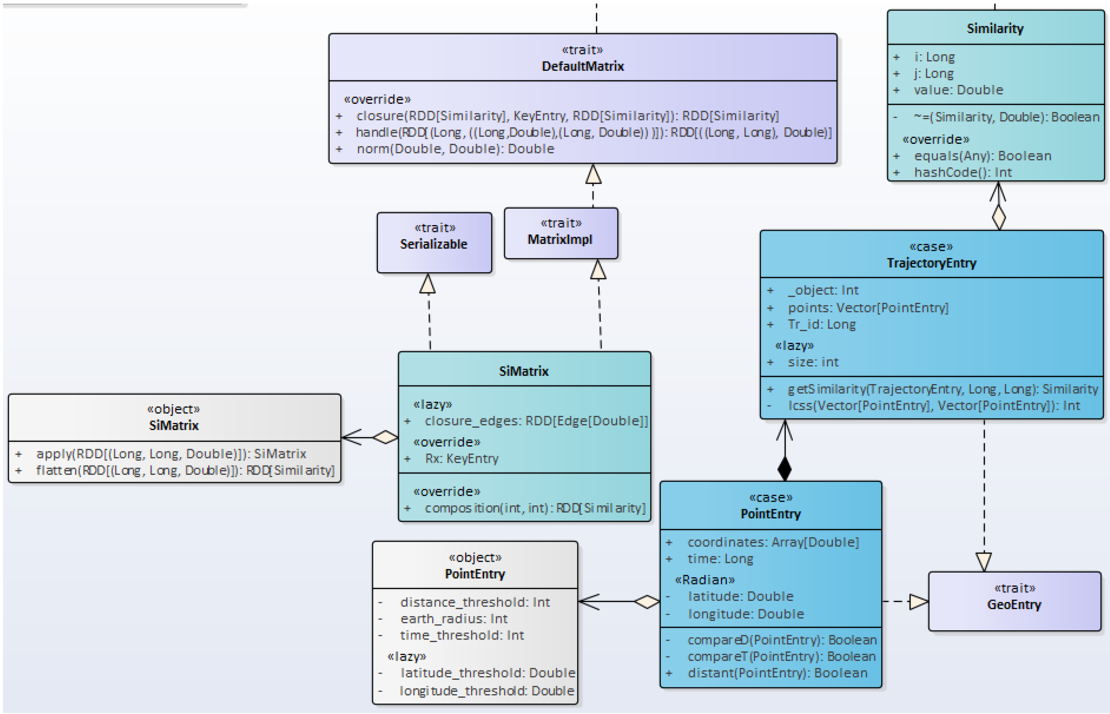
4.1. The Project’s Class Diagrams

The project integrates the Scala Stackable Trait Pattern. In detail, we provide an abstraction called AbstractMatrix. It is an abstract class holding the abstract definition of all the operations needed to achieve the transitive closure. Then, different traits override specific abstract definitions to customize the behavior. Traits extend java interfaces to provide much richer functionalities. In our case, traits extend the AbstractMatrix with specific behavior; they are denoted mixins, e.g., the MaxMinNorm overrides the norm function into computing the minimum of the inputs and the Seminaive mix overrides the closure algorithm definition. They can only be extended by classes already extending the AbstractMatrix. Also, the AbstracMatrix has a companion object defining a specific KeyEntry Type and a static ireverse operation which reverses the Similarity class entries for the closure’s composition join. The Similarity class resembles Spark’s MatrixEntry case class in the Spark MLlib library. However, it is not a case class and it overrides both the equals and hashCode operations to provide specific comparison behavior. The rationale behind this class is that we observed an anomaly when computing the transitive closure. More specifically, the transitive closure computing time was very large. After observing the computing process, we found out that when subtracting the results of the past and present, iterations in the closure’s similarities were not considered equal because of their weights. Although, the weights differed from each other in a precision of ${10}^{-9}$. This fact led us to provide our own comparison strategy with a custom precision of ${10}^{-3}$ integrated in the Similarity class.

The abstraction is extended by another trait DefaultMatrix. Like the name suggests, the trait provides default behavior for the abstract definition. This has made it possible to leverage the abstract operations without defining a default behavior for each class. As the Figure 2 shows, the class SiMatrix can leverage the AbstractMatrix operation without having to override them. This is our approach extension of the stackable trait. Furthermore, Scala traits support self types. Meaning that a trait can only be extended by a subclass of the specified type. Which is why we implemented a MatrixImpl, a self type of the DefaultMatrix, adding a restriction to the inheritance strategy. The concrete class SiMatrix extends both the DefaultMatrix and the Serializable traits to respectively be able to leverage all the AbstractMatrix traits and to execute spark stages. Note that in the other traits, we did not override the composition operation because we provided a concrete definition in the lowest level SiMatrix class. To create the SiMatrix objects, we needed a factory pattern. Fortunately, the factory pattern is simplified in Scala by companion objects (A companion object of a specific class in Scala has the same name as the class and it can access the private variables and operations of the class). The SiMatrix is a companion object providing the factory method for instantiating its relative class. An extract of the apply method is described in Algorithm 2. The function is a higher order function based on currying. The first function takes as input the distributed similarities and outputs a function that takes the alpha threshold used for the partitioning, the chosen t-norm and transitive closure algorithm. Then, depending on the t-norm and closure algorithm it instantiates the SiMatrix class while specifying the traits to be mixed in. Note that the order of the trait is important. Scala is based on linearization principle, the last trait is the first to be extended. Hence, the name stackable trait pattern. It is like a stack of patterns where the first one to be extended is actually the last.

Algorithm 2: The SiMatrix companion object apply method.

The apply method of the SiMatrix object leverages the flatten function to create a reverse duplicate of the entries and return an iterator of the couple which will be flattened by Spark’s flatMap operation. Now, for computing the closure, we specified two traits Seminaive and Smart related respectively to the semi-naive and smart algorithm. The difference between the two is that at each iteration the first considers the initial relation when computing the composition, while the second considers the same relation related to the current iteration. This led us to define a curried function for each trait with default parameters. In the Seminaive trait Algorithm 3, we specify that Rx equals the predefined Rx in the AbstractMatrix, which gets overridden in the SiMatrix class. The last function in the closure curried form computes the composition of the past specified parameters Ri and Rx. This reflects the high potential of Scala’s higher order function into simplifying highly complex computations. At the heart of the closure function, we check if the current Rj equals the past iteration Ri. If the preposition holds, we return Ri; otherwise, we call the closure again in a recursive manner with Ri as Rj and the other parameters as default ones. As for the Smart trait Algorithm 4; we change Rx into a KeyEntry value returned by calling the ireverse function on the first parameter Ri. Note that to compute the transitive closure, we consider the type KeyEntry which reflects the RDD[(Long,(Long, double))] type. The first relation gets its columns extracted and joined with the rows of the second relation which are extracted by the ireverse function. The composition is overridden in the SiMatrix class (please see the Algorithm 5). In particular, the composition calls the handle function which in the same manner calls the norm function. Hence, the order of the mixins is very important.

Algorithm 3: The SemiNaive trait.

Algorithm 4: The Smart trait.

Algorithm 5: The overridden composition method in the SiMatrix class.

To compute the similarities of the trajectories, we defined a trait GeoEntry that gets extended by the PointEntry and TrajectoryEntry case classes. Case classes in scala are serialized by default, their constructor parameters become accessible variables and functions like equals and hashCode are overridden. They are related to the Value Object Pattern. The TrajectoryEntry class is composed by objects of the PointEntry class. The similarities of the points gets computed by the getSimilarity function which call the recursive function lcss both defined in the TrajectoryEntry class. The points gets compared respectively by their time and distance by the functions defined in the PointEntry class. The order of the comparison is important to reduce additional time overhead. At last, the closure can be accessed via the closure_edges immutable lazy variable. In particular, the laziness reflects the Lazy initialization Pattern where the variable gets instantiated on access. The overall pipeline of the process is described in the next subsection with activity diagrams.

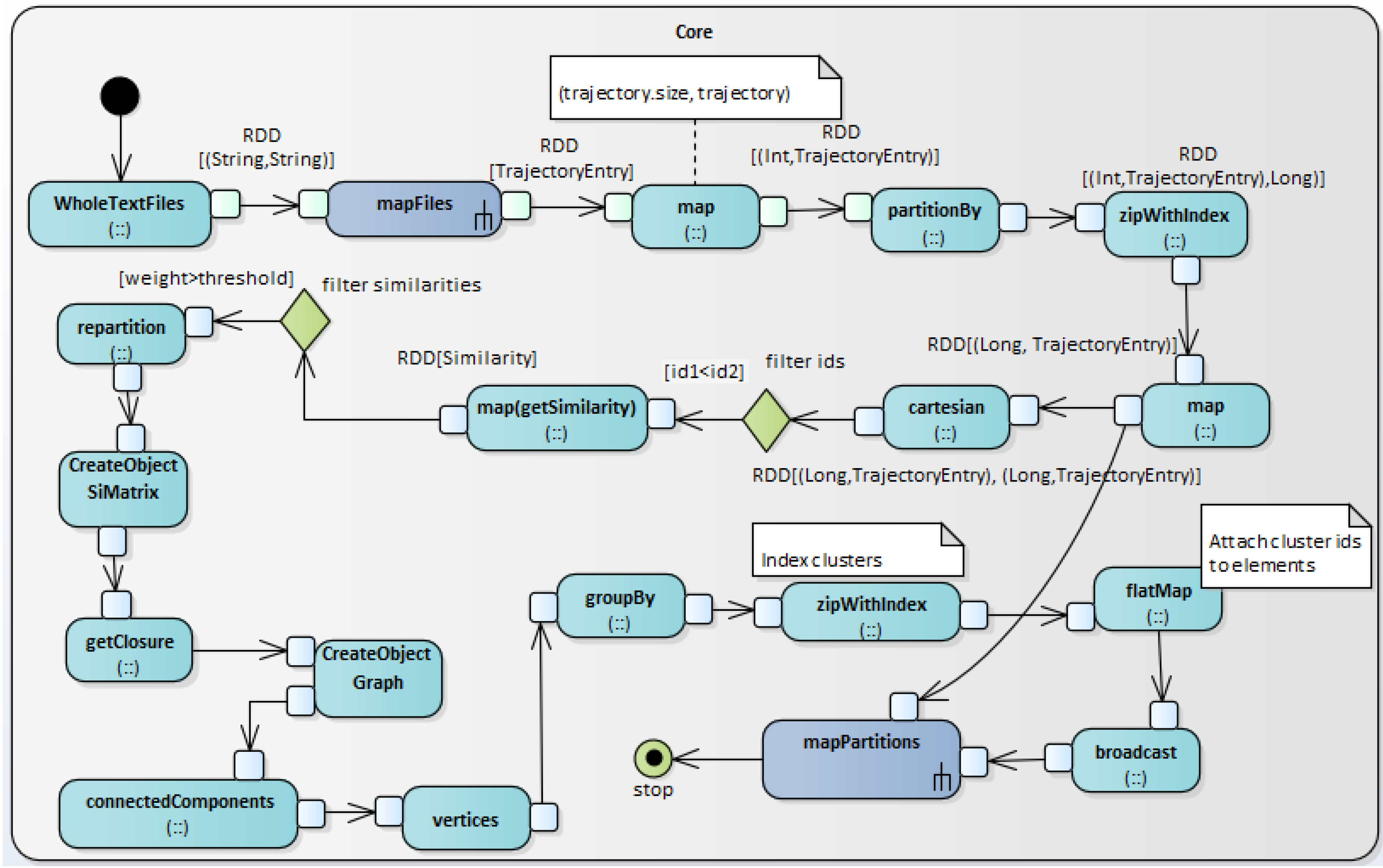
4.2. The Overall Execution Pipeline

The activity in Figure 3 reflects the overall process. All the actions in the diagram are distributed. First, we leverage Spark’s wholeTextFiles operation to read the different directories. Also, we specify the number of partitions. While experimenting, we observed that if we specify n partitions we get 2*n ones. After reading the files, we use the Spark’s map operation to retrieve the trajectory from each file. Spark’s map function is a higher order function taking as a parameter another function which gets specified by us. Figure 4 illustrates the trajectories’ creation process. Each file is handled in a distributed manner; however, each line of the files is handled sequentially to create instances of the PointEntry class.

Afterward, we evaluated the system and we observed a relatively large time overhead. This led us to specify our own custom partitioning strategy based on the trajectories’ sizes. The strategy is implemented in the LoadPartitioner class which extends Spark’s Partitioner abstract class. The partitioner has to override the functions numPartitions and getPartition which return the id of the chosen partition. Details are in Algorithm 6, the main idea behind the partitioning strategy is to return the partition with the lowest size. The size of the partitions is not defined by the number of the trajectories, but the size of the points in the trajectories. The efficiency of the logic is provided in Section 5.

Algorithm 6: The LoadPartitioner class.

Now that the partitions got repartitioned successfully, we zip each trajectory with a unique identifier. Then, we suppress the trajectories’s sizes and conduct the cartesian product to assemble the similarities’ elements. After the cartesian product, we conduct a special filter. This filter enables us to reduce the load to more than the half of the overall couples. Instead of computing the similarities of $n^2$ elements, we compute only $A_n^1+A_{n-1}^1+\dots +A_1^1-n$. This is achieved by considering only the couples where the first trajectory’s id is inferior than the second. Because the relation is a fuzzy proximity relation, we do only have to compute $R(x,y)$ not also $R(y,x)$. Also, we do not have to consider $R(x,x)$ because it equals 1. Next, we compute the similarities and conduct a filter to suppress the similarities with a weight inferior than the chosen $\alpha$-level. The importance of repartitioning the similarities after the filter is proven in the Section 5. After repartitioning, we construct the SiMatrix object and compute the closure. For the clustering, we consider the max–min transitivity and extract the clusters by defining the connected elements of the created Graph object belonging to the Spark’s GraphX library. All the extracted clusters form maximum cliques. Now that the clusters are identified, we index each element by its relative cluster, collect and broadcast the identifiers in a Map type form. The rationale behind this broadcast is to reduce the time overhead for the join. Because Spark’s joins require shuffle of the data and this can cost a lot of time. However, the broadcast enables us to cache the identifiers in each worker. The join and persistence of the objects are explained in the Figure 5.

Instead of handling each element, we handle each partition to reduce the number of database connections. For persisting the results, we leverage the Reactive MongoDB Driver. First, a driver object, a database and a collection object get created. Their creation is conducted in an asynchronous manner. This means that we do not actually get the real objects. Instead, we get Scala’s Futures. After the completion of the futures, we iterate over the trajectories. For each trajectory, we get its cluster id by looking up its id in the broadcasted map. Then, we create a bson object and call the insert operation of the collection. The operation is conducted asynchronously in a non-blocking manner. Consequently, other bson objects are being created and inserted in the same time. This is achieved by configuring the spark.task.cpus parameter to the desired number of threads per task. Then, we assemble the futures in a sequence and await its completion. In the end, we destroy the driver and return the final write result to declare the end of the task.

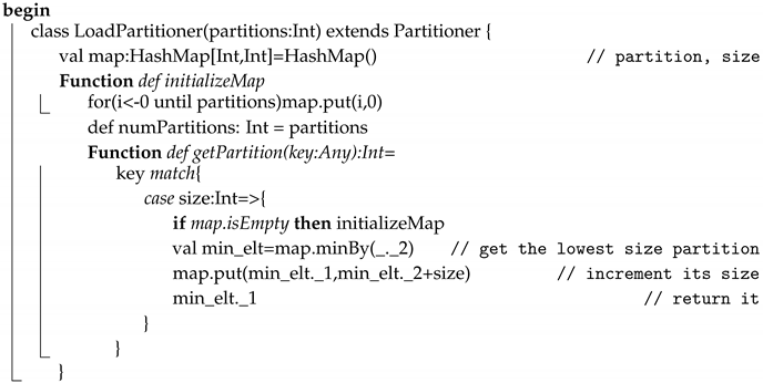5. Results and Discussions

In the experiments, we deployed a cluster of 6 workers. The master and a worker have 8 cores and respectively 8 and 6 GB in the RAM, while the others have 4 cores and 4 GB memory. In the configuration, we specified the spark.driver.memory and spark.executor.memory to respectively equal 4000 MB and 2000 MB. First, in the experience we observed a large set of StackOverFlowError exceptions. This is explained by the recursive call of the lcss in the executors. To resolve this issue, we increased the maximum stack size in the executors by setting an extra java option in the executors’ configurations with spark.executor.extraJavaOptions set to -Xss40M. This increases the default maximum stack size into 40 MB.

While evaluating the performance of the conventional pipeline, we observed a large time overhead. When we checked the metrics in the SparkUI, we observed a large disturbance in the tasks visible in Figure 6. This fact is explained by the uneven complexity of the trajectories. To resolve this issue, we proposed our own partitioning strategy already explained in Section 4. After integrating the LoadPartitioner strategy, we observed the balanced workload illustrated in Figure 7. Moreover, we evaluated the performance of the system and plotted the results in Figure 8. The results provide the empirical evidence of the high efficiency of our partitioning strategy in reducing the computation time by equally balancing the workloads.

After conducting the filter of the similarities, we additionally observed a time overhead. The SparkUI reflected the Figure 9. In the figure, we observed a large number of tasks which are executed in a very short time, a matter of milliseconds. Hence, each partition contains a very limited number of elements compared to the past load before the filter. To resolve this additional time load, we conducted a repartitioning just after the filter and observed the difference in Figure 10. The execution time of the two possibilities is plotted in Figure 11. We acknowledge that both the partitionBy and repartitioning stages may cause an additional overhead because of the shuffle behavior. But over unbalanced loads and after a large filter operation, they are indispensable to reduce the execution time. In particular, the repartitioning strategy after the filter as can be seen in Figure 10 reduces and reassembles the partitions into a single executor. This fact highly reduces additional NetworkIO overhead.

6. Conclusions

We provide a pipeline for clustering trajectories by resolving the LCSS problem. The clustering is achieved via the max–min transitive closure of the fuzzy proximity relation. Clusters are yielded based on a predefined $\alpha$-level. Spark is exploited to distribute the execution of the pipelines’ tasks. Details about the implementation of the different stages are yielded. To reduce the execution time, we studied the repartitioning effect over the conventional pipeline. Then, we proposed a new partitioning logic, which resolves the load balancing issue and integrated the repartitioning after the filtering of the similarities. Our results prove the efficiency of our partitioning strategy and the repartitioning in reducing the computation time. Moreover, we integrated the asynchronous Reactive MongoDB Driver as a first step into studying the behavior of spark in the asynchronous boundaries. We acknowledge that this integration needs further evaluation. In addition, we are currently working on two projects. The first aims to integrate a fully distributed algorithm for defining the clusters in the max–product and max–delta fuzzy similarity relations. The second is to employ a new iterative algorithm that exploits Spark’s GraphX integration of Pregel. This last will be able to highly reduce the time overhead for computing the transitive closure of a fuzzy subjective similarity relation.

Computer Code

The project’s Scala code can be retrieved from our github repository: https://github.com/strangex/spark-transitive-closure.

References

- Zheng, Y.; Zhang, L.; Xie, X.; Ma, W.Y. Mining Interesting Locations and Travel Sequences From GPS Trajectories. In Proceedings of the International conference on World Wide Web 2009, Madrid, Spain, 20–24 April 2009. [Google Scholar]
- Zheng, Y.; Li, Q.; Chen, Y.; Xie, X.; Ma, W.Y. Understanding Mobility Based on GPS Data. In Proceedings of the Ubicomp 2008, Seoul, Korea, 21–24 September 2008. [Google Scholar]
- Zheng, Y.; Xie, X.; Ma, W.Y. Geolife: A collaborative social networking service among user, location and trajectory. IEEE Data Eng. Bull. 2010, 33, 32–39. [Google Scholar]
- Magdy, N.; Sakr, M.A.; Mostafa, T.; El-Bahnasy, K. Review on trajectory similarity measures. In Proceedings of the 2015 IEEE Seventh International Conference on Intelligent Computing and Information Systems (ICICIS), Cairo, Egypt, 12–14 December 2015; pp. 613–619. [Google Scholar]
- Zheng, V.W.; Cao, B.; Zheng, Y.; Xie, X.; Yang, Q. Collaborative Filtering Meets Mobile Recommendation: A User-Centered Approach. In Proceedings of the AAAI, Atlanta, GA, USA, 11–15 July 2010; Volume 10, pp. 236–241. [Google Scholar]
- Ioannidis, Y.E. On the computation of the transitive closure of relational operators. In Proceedings of the VLDB, Berkeley, CA, USA, 25–28 August 1986; Volume 86, pp. 403–411. [Google Scholar]
- Brodie, M.L.; Mylopoulos, J. On Knowledge Base Management Systems: Integrating Artificial Intelligence and Database Technologies; Springer Science & Business Media: New York, NY, USA, 2012. [Google Scholar]
- Zadeh, L.A. Fuzzy Logic and Its Applications; Springer: New York, NY, USA, 1965. [Google Scholar]
- Yang, M.S. A survey of fuzzy clustering. Math. Comput. Model. 1993, 18, 1–16. [Google Scholar] [CrossRef]
- Yao, J.; Dash, M.; Tan, S.; Liu, H. Entropy-based fuzzy clustering and fuzzy modeling. Fuzzy Sets Syst. 2000, 113, 381–388. [Google Scholar] [CrossRef]
- Boulmakoul, A.; Zeitouni, K.; Chelghoum, N.; Marghoubi, R. Fuzzy structural primitives for spatial data mining. Complex Syst. 2002, 5, 14. [Google Scholar]
- Kondruk, N. Clustering method based on fuzzy binary relation. East.-Eur. J. Enterp. Technol. 2017, 2. [Google Scholar] [CrossRef]
- Tamura, S.; Higuchi, S.; Tanaka, K. Pattern classification based on fuzzy relations. IEEE Trans. Syst. Man Cybern. 1971, SMC-1, 61–66. [Google Scholar] [CrossRef]
- Yang, M.S.; Shih, H.M. Cluster analysis based on fuzzy relations. Fuzzy Sets Syst. 2001, 120, 197–212. [Google Scholar] [CrossRef]
- Liang, G.S.; Chou, T.Y.; Han, T.C. Cluster analysis based on fuzzy equivalence relation. Eur. J. Oper. Res. 2005, 166, 160–171. [Google Scholar] [CrossRef]
- Houtsma, M.A.; Apers, P.M.; Ceri, S. Distributed transitive closure computations: The disconnection set approach. In Proceedings of the VLDB, Brisbane, Queensland, Australia, 13–16 August 1990; Volume 90, pp. 335–346. [Google Scholar]
- Houtsma, M.A.; Apers, P.M.; Schipper, G.L. Data fragmentation for parallel transitive closure strategies. In Proceedings of the IEEE Ninth International Conference on Data Engineering, Vienna, Austria, 19–23 April 1993; pp. 447–456. [Google Scholar]
- Gribkoff, E. Distributed Algorithms for the Transitive Closure. 2013. Available online: https://pdfs.semanticscholar.org/57fd/5969b2a454c90b57b12c49e90847fee079a8.pdf (accessed on 19 January 2019).
- Boulmakoul, A.; Maguerra, S.; Karim, L.; Badir, H. A Scalable, Distributed and Directed Fuzzy Relational Algorithm for Clustering Semantic Trajectories. In Proceedings of the Sixth International Conference on Innovation and New Trends in Information Systems, Casablanca, Morocco, 24–25 November 2017. [Google Scholar]
- Maguerra, S.; Boulmakoul, A.; Karim, L.; Badir, H. Scalable Solution for Profiling Potential Cyber-criminals in Twitter. In Proceedings of the Big Data & Applications 12th Edition of the Conference on Advances of Decisional Systems, Marrakech, Morocco, 2–3 May 2018. [Google Scholar]
- Li, H.; Liu, J.; Wu, K.; Yang, Z.; Liu, R.W.; Xiong, N. Spatio-temporal vessel trajectory clustering based on data mapping and density. IEEE Access 2018, 6, 58939–58954. [Google Scholar] [CrossRef]
- Yi, D.; Su, J.; Liu, C.; Chen, W.H. Trajectory Clustering Aided Personalized Driver Intention Prediction for Intelligent Vehicles. IEEE Trans. Ind. Inform. 2018. [Google Scholar] [CrossRef]
- Zadeh, L.A. Fuzzy sets. Inf. Control 1965, 8, 338–353. [Google Scholar] [CrossRef]
- Bezdek, J.C.; Harris, J.D. Fuzzy partitions and relations; an axiomatic basis for clustering. Fuzzy Sets Syst. 1978, 1, 111–127. [Google Scholar] [CrossRef]
- Boulmakoul, A.; Karim, L.; Lbath, A. Moving object trajectories meta-model and spatio-temporal queries. arXiv, 2012; arXiv:1205.1796. [Google Scholar] [CrossRef]
- Cook, J.D. Converting Miles to Degrees Longitude or Latitude. 2009. Available online: https://www.johndcook.com/blog/2009/04/27/converting-miles-to-degrees-longitude-or-latitude/ (accessed on 30 November 2018).
- Hirschberg, D.S. A linear space algorithm for computing maximal common subsequences. Commun. ACM 1975, 18, 341–343. [Google Scholar] [CrossRef]
© 2019 by the authors. Licensee MDPI, Basel, Switzerland. This article is an open access article distributed under the terms and conditions of the Creative Commons Attribution (CC BY) license (http://creativecommons.org/licenses/by/4.0/).
Share and Cite
Maguerra, S.; Boulmakoul, A.; Karim, L.; Badir, H. A Distributed Execution Pipeline for Clustering Trajectories Based on a Fuzzy Similarity Relation. Algorithms 2019, 12, 29. https://doi.org/10.3390/a12020029
Maguerra S, Boulmakoul A, Karim L, Badir H. A Distributed Execution Pipeline for Clustering Trajectories Based on a Fuzzy Similarity Relation. Algorithms. 2019; 12(2):29. https://doi.org/10.3390/a12020029
Chicago/Turabian StyleMaguerra, Soufiane, Azedine Boulmakoul, Lamia Karim, and Hassan Badir. 2019. "A Distributed Execution Pipeline for Clustering Trajectories Based on a Fuzzy Similarity Relation" Algorithms 12, no. 2: 29. https://doi.org/10.3390/a12020029
APA StyleMaguerra, S., Boulmakoul, A., Karim, L., & Badir, H. (2019). A Distributed Execution Pipeline for Clustering Trajectories Based on a Fuzzy Similarity Relation. Algorithms, 12(2), 29. https://doi.org/10.3390/a12020029