Abstract
We propose a new iterative greedy algorithm to reconstruct sparse signals in Compressed Sensing. The algorithm, called Conjugate Gradient Hard Thresholding Pursuit (CGHTP), is a simple combination of Hard Thresholding Pursuit (HTP) and Conjugate Gradient Iterative Hard Thresholding (CGIHT). The conjugate gradient method with a fast asymptotic convergence rate is integrated into the HTP scheme that only uses simple line search, which accelerates the convergence of the iterative process. Moreover, an adaptive step size selection strategy, which constantly shrinks the step size until a convergence criterion is met, ensures that the algorithm has a stable and fast convergence rate without choosing step size. Finally, experiments on both Gaussian-signal and real-world images demonstrate the advantages of the proposed algorithm in convergence rate and reconstruction performance.
1. Introduction
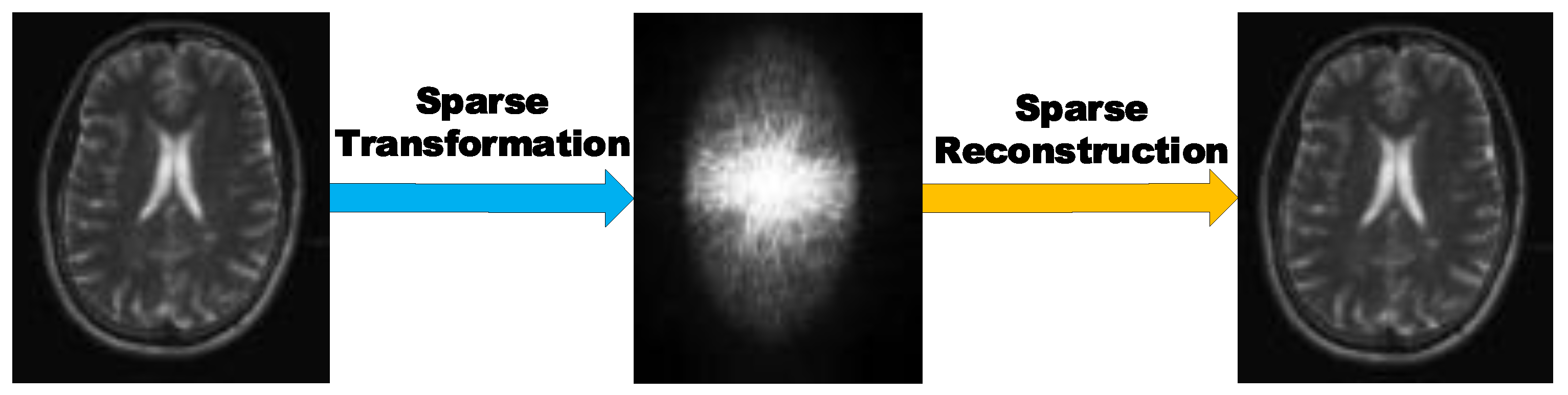
As a new sampling method, Compressed Sensing (CS) has received broad research interest in signal processing, image processing, biomedical engineering, electronic engineering and other fields [1,2,3,4,5,6]. In particular in magnetic resonance image (MRI) processing, CS technology greatly improves the efficiency of MRI processing (Figure 1). By exploiting the sparse characteristics of signals, CS can accurately reconstruct sparse signals from significantly fewer samples than required in the Shannon-Nyquist sampling theorem [7,8].
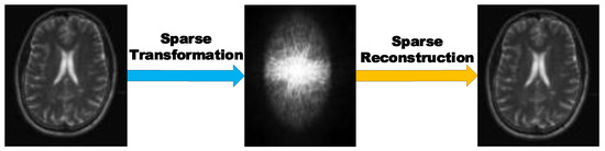
Figure 1.
Application of Compressed Sensing in Magnetic Resonance Images (MRI) [4].
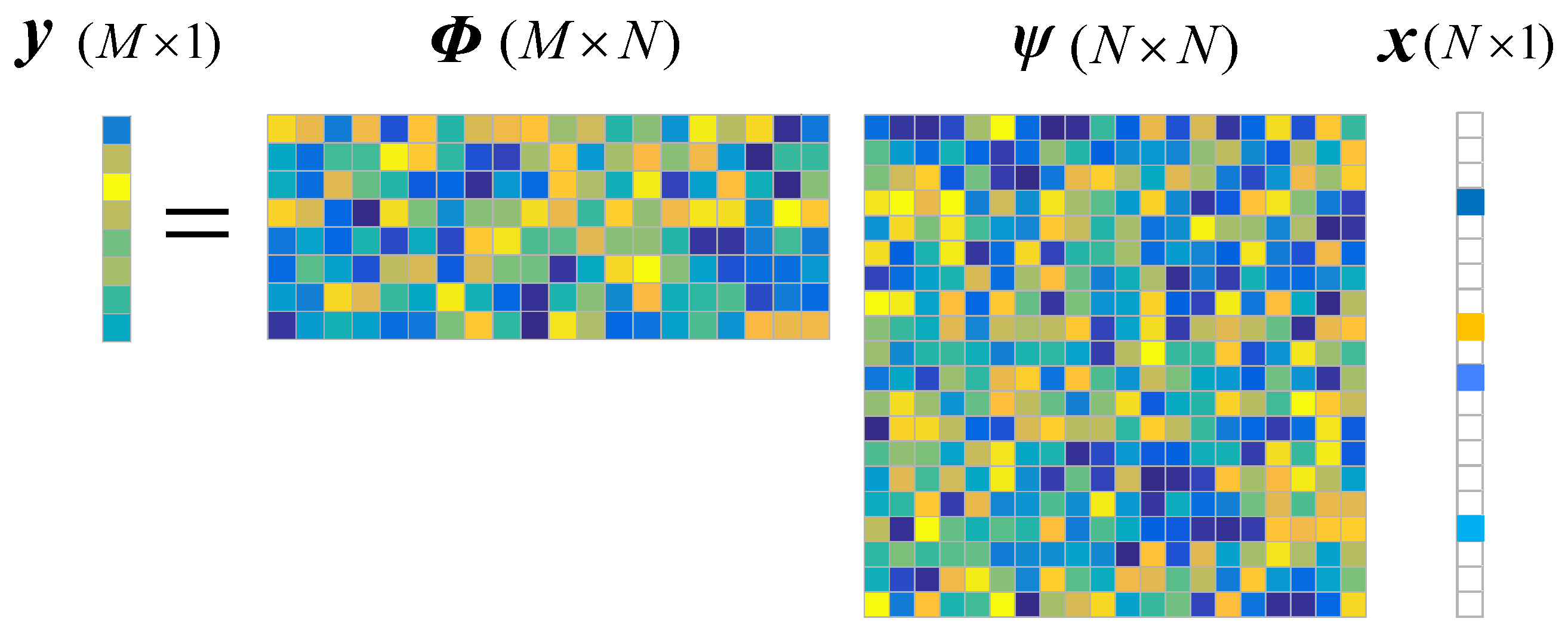
Assume that a signal is s-sparse in some domain . This means , and has at most nonzero entries. This system can be measured by a sampling matrix : , where is called measurement vector, is the so-called measurement matrix. The CS model is shown in Figure 2. If is incoherent with , the coefficient vector can be reconstructed exactly from a few measurements by solving the undetermined linear system with constraint , i.e., solving the following norm minimization problem:
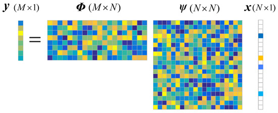
Figure 2.
Compressed Sensing model with .
As a combinatorial optimization problem, the above norm optimization is NP-hard [8]. One way to solve such problem is to transform it into a norm optimization problem:
Since norm-based problem is convex, some methods such as basis pursuit (BP) [7] and LASSO [9] are usually employed to solve the norm minimization in polynomial time. The solutions obtained by these algorithms can well approximate the exact solution of (1). However, their computational complexity is too highly impractical for many applications. As a relaxation of the norm optimization, the norm for CS reconstruction has attracted extensive research interest, and the problem can be formulated as the following optimization problem:
where denotes the norm of . There are many methods have been developed to solve such problem [10,11,12,13]. Many studies have shown that using norm for requires fewer measurements and has much better recovery performance than using norm [14,15]. However, norm leads to a non-convex optimization problem which is difficult to solve efficiently.
Sparse signals can be quickly recovered by these algorithms while the measurement matrix satisfying the so-called restricted isometry property (RIP) with a constant parameter. A measurement matrix is said to satisfy the s-order RIP if for any s-sparse signal
where . Commonly used sampling matrices include Gaussian matrices, random Bernoulli matrices, partial orthogonal matrices, etc. The measurement matrices consisting of these sampling matrices and orthogonal basis usually satisfy the RIP condition with a high probability [16].
The core ideas of this paper include: (1) by combining the steps of HTP and CGIHT in each iteration, a new algorithm called Conjugate Gradient Hard Thresholding Pursuit (CGHTP) is presented; (2) by alternatively selecting a search direction from the gradient direction and the conjugate direction to improve the convergence rate of the iterative procedure; (3) furthermore, an adaptive step size selection strategy similar to that in normalized iterative hard thresholding (NIHT) is adopted in CGHTP algorithm, which eliminates the effect of step size on the convergence of HTP algorithm.
The remainder of the paper is organized as follows. Section 2 reviews related work on iterative greedy algorithms for CS. Section 3 gives the key ideas and description of the proposed algorithm. The convergence analysis of the CGHTP algorithm is given in Section 4. Some simulation experiments to verify the empirical performance of the CGHTP algorithm is carried out in Section 5. Finally, the conclusion of this paper is presented in Section 6.
Notations: in this paper, ∅ represents an empty set. denotes the inner product of the vector and . denotes an operator that sets all but the largest s absolute value of . is denoted to take the index set of nonzero entries of . Let . Let denote a subvector consisting of elements extracted from that indexed by the elements in T. denotes a submatrix that consists of the columns of with indices . denotes the transpose of . stands for a unit matrix whose size depends on the context. In addition, let denote the sampling ratio.
2. Literature Review
In the past decade, a series of iterative greedy algorithms has been proposed to directly solve Equation (1). These algorithms have been attracting increased attention due to their low algorithm complexity and good reconstruction performance. According to the support set selection strategy used in the iteration process, we can roughly classify the family of iterative greedy algorithms into three categories.
(1) orthogonal matching pursuit (OMP) [17]-based OMP-like algorithms, such as compressive sampling matching pursuit (CoSaMP), subspace pursuit (SP) [18], regularized orthogonal matching pursuit (ROMP) [19], generalized orthogonal matching pursuit (GOMP) [20], sparsity adaptive matching pursuit (SAMP) [21], stabilized orthogonal matching pursuit (SOMP) [22], perturbed block orthogonal matching pursuit (PBOMP) [23] and forward backward pursuit (FBP) [24]. A common feature of these algorithms is that in each iteration, a support set is determined to approximate the correct support set according to the correlation value between the measurement vector and the columns of .
(2) iterative hard thresholding (IHT)-based IHT-like algorithms, such as NIHT, accelerated iterative hard thresholding (AIHT) [25], conjugate gradient iterative hard thresholding (CGIHT) [26,27]. Unlike the OMP-like algorithm, the approximate support set for the nth iteration of IHT-like algorithms is determined by the value of , which is closer to the correct support set than using the values of [28].
(3) algorithms composed of OMP-like and IHT-like algorithms, such as Hard Thresholding Pursuit (HTP) [28,29], generalized hard thresholding pursuit (GHTP) [30], regularized HTP [31], Partial hard thresholding (PHT) [32] and subspace thresholding pursuit (STP) [33]. OMP-like algorithms use least squares to update sparse coefficients in each iteration, which plays a role in debiasing and makes it approach the exact solution quickly. However, it is well known that the least squares are time-consuming, which leads to a high complexity of single iteration. The advantage of IHT-like algorithms are the simple iteration operation and good support set selection strategy, but it needs more iterations. By combining the OMP-like algorithm and the IHT-like algorithm, these algorithms absorb the advantages of the above two kinds of algorithms, and have strong theoretical guarantees and good empirical performance [29].
Among the above algorithms, CoSaMP and SP do not provide a better theoretical guarantee than the IHT algorithm, but their empirical performance is better than IHT. The simple combination of CoSaMP and IHT algorithm lead to the HTP algorithm whose convergence requires fewer number of iterations than IHT algorithm. However, the reconstruction performance of HTP is greatly affected by the step size and an optimal step size is difficult to determine in practical applications, which may cause the HTP to converge slowly when selecting an inappropriate step size. Furthermore, although the HTP algorithm only requires a small number of iterations to converge to the exact vector , it only uses a single gradient descent direction as the search direction in iterative progress, which may not be the best choice for general optimization problems. In [26], conjugate gradient method was used to accelerate the convergence of IHT algorithm due to its fast convergence rate. In this paper, inspired by the HTP algorithm and CGIHT algorithm, the operations of these two algorithms in each iteration is combined to take advantage of both.
In this paper, we first introduce the idea of the CGHTP algorithm, then analyze the convergence of the proposed algorithm, and finally validate the proposed algorithm with synthetic experiments and real-world image reconstruction experiments.
3. Conjugate Gradient Hard Thresholding Pursuit Algorithm
Firstly, we make a simple summary of the HTP algorithm and the CGIHT algorithm to facilitate an intuitive understanding of the proposed algorithm. The pseudo-codes of HTP and CGIHT are shown in Algorithms 1 and 2, respectively. In [20], the debiasing step in the OMP-like algorithms and the estimation step in the IHT-like algorithms are coupled in an algorithm to form the HTP algorithm. The HTP algorithm has excellent reconstruction performance as well as strong theoretical guarantee in terms of the RIP. Optimizing search direction in each iteration is the main innovation of HTP algorithm. It fully considers that in the iterative process, when the subspace determined by the support set is consistent, the conjugate gradient (CG) method [23] can be employed to accelerate the convergence rate. Two versions of CGIHT algorithms for CS are provided in [19], one of them, the algorithm called CGIHT restarted for CS is summarized in Algorithm 2. The iteration procedures of CGIHT and CGIHT restarted differ in their selection of search directions. CGIHT algorithm uses the conjugate gradient respect to as the search direction in all iteration, while CGIHT restarted determines the search direction according to whether the support set of the current iteration is equal to that of the previous iteration.
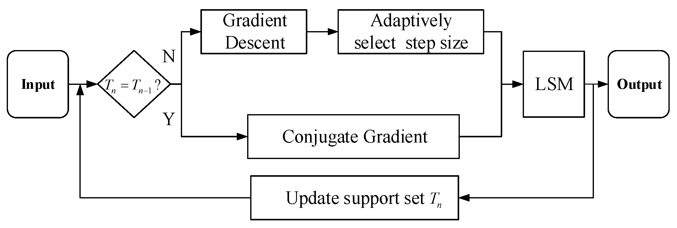
Inspired by the respective advantages of HTP and CGIHT algorithms, we present the CGHTP algorithm in this section. A simple block diagram of the CGHTP algorithm can be seen in Figure 3. The algorithm enters an iterative loop after inputting the initialized data. The loop process updates the and support set in two alternative ways, one of which is the combination of the gradient descent method and the adaptive step size selection method, and the other is the CG method. The selection criteria for these two ways is to determine whether the support sets of two adjacent iterations are equal. If the support set of the previous iteration is equal to that of the current iteration, then the gradient descent method is used. If not, the CG method is used [34]. All candidate solutions and candidate support sets obtained through these ways are finally updated by the least square method.
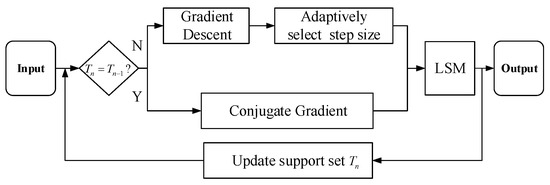
Figure 3.
Block diagram of CGHTP algorithm. is the support set of in the nth iteration, “LSM” denotes least square method.
The main characteristic of the proposed CGHTP algorithm is that the support set selection strategy of HTP is combined with the acceleration strategy of CGIHT restarted algorithm in one algorithm. The main steps of CGHTP are listed in Algorithm 3. Similar to CGIHT, CGHTP is initialized with , . The main body of CGHTP mainly includes the following steps. In Step 1), the gradient direction of the cost function [16] in the current iteration is solved to calculate the subsequent step size . In Step 2), if has a different support from the previous estimate, i.e., , similar to the convergence criterion used in NIHT algorithm, is used to check whether the step size is smaller than it, where c is a small fixed constant and . If this holds, continue to run the next steps. Otherwise the step size is continuously reduced by looping until the convergence criterion is met, here . In Step 3), if , the CG direction is used as the search direction. Finally, Step 4) updates by solving a least square problem.
Compared to the HTP algorithm, the CGHTP algorithm provides two search directions in the iterative process, including the gradient direction of the cost function and the CG direction . According to whether the support sets of the previous and current iterations are equal, one of the two directions is selected as the search direction. In addition, then the support set is updated by solving a least square problem. In addition, CGHTP provides a way to choose the best step size while ensuring convergence.
The HTP algorithm uses the gradient direction as the search direction, which has a linear asymptotic convergence rate related to , where is the condition number of the matrix . Owing to the superlinear asymptotic convergence speed with a rate given by [24], conjugate gradient method has been applied to accelerate the convergence rate in CGIHT algorithm. CGHTP draws on the advantages of the CGIHT algorithm. If , it means that the correct support set is identified and the submatrix is no longer changed, CG method is applied to solve the overdetermined system , and the convergence rate may be superlinear with a rate given by .
| Algorithm 1 [20] Hard Thresholding Pursuit |
| Input: , , s Initialization: , . for each iteration do 1) 2) 3) 4) update the residual until the stopping criteria is met end for |
| Algorithm 2 [19] Conjugate Gradient Iterative Hard Thresholding restarted for Compressed Sensing |
| Input: , , s Initialization: , , , . for each iteration do 1) (compute the gradient direction) 2) if then else (compute orthogonalization weight) end 3) (compute conjugate gradient direction) 4) (compute step size) 5) , until the stopping criteria is met end for |
| Algorithm 3 Conjugate Gradient Hard Thresholding Pursuit |
| Input: , , s, Initialization: , , , . for each iteration do 1) (compute gradient direction) 2) if then if then execute loop until (adaptively select step size) , end end 3) if then (compute conjugate gradient direction) (compute optimal step size) , end 4) end for Output: , |
4. Convergence Analysis of CGHTP
In this section, we analyze the convergence of the proposed algorithms. We give a simple proof that the CGHTP algorithm converges to the exact solution of (1) after a finite number of iterations when the measurement matrix satisfies some conditions.
In Algorithm 3, when and , the iterative process of the CGHTP algorithm is equivalent to the HTP algorithm. Similar to Lemma 3.1 in [20], we obtain the following lemma:
Lemma 1.
The sequences defined by CGHTP eventually periodic.
Theorem 1.
The sequencegenerated by CGHTP algorithm converges toin a finite number of iterations, wheredenotes the exact solution of (1)
The proof of Theorem 1 is partitioned here into two steps. The first step is that when the current support set is not equal to the previous support set, the orthogonal factor is equal to 0. At this time, the CGHTP algorithm reduces to the HTP algorithm, so their convergence is the same. The second step is that when the two support sets are equal, the step size is related to the orthogonal factor and the CG direction. Detailed proof is given below.
Proof of Theorem 1.
When , according to Algorithm 3, and , since , one has
It is clear that is a better approximation to than is, so . By expanding the squares, we can obtain , substituting this into (5), one has
substituting into inequality (6), one can show that
Since , the right side of (7) is less than 0. This implies that the cost function is nonincreasing when , hence it is convergent.
In the case of , for the overdetermined linear system , since is a positive definite matrix, CG method for solving such problem has the convergence rate as:
where . The submatrix satisfies the RIP condition: . It is easy to get that . Then (8) can be rewritten as
where . From Lemma 1, since the sequence is eventually periodic, it must be eventually constant, which implies that and for n large enough. In summary, the CGHTP algorithm is convergent. □
5. Numerical Experiments and Discussions
In this section, we verify the performance of the proposed algorithm by Gaussian-signal reconstruction experiments and real-world images reconstruction experiments. This section compares the reconstruction performance of HTP (with several different step sizes), CGIHT, and CGHTP with parameter . All experiments are tested in MATLAB R2014b, running on a Windows 10 machine with Intel I5-7500 CPU 3.4 GHz and 8GB RAM.
5.1. Gaussian-Signal Reconstruction
In this subsection, we construct an random Gaussian matrix as the measurement matrix with entries drawn independently from Gaussian distribution. In addition, we generate an s-sparse signal of length , and each nonzero element of this signal is chosen at random and drawn from standard Gaussian distribution. Here, we define the subsampling rate as . In each experiment, we let HTP execute with four different : , , and , where denotes the step size with which HTP has the optimal empirical performance. In all the tests in this section, each experiment is repeated 500 times independently. To evaluate the performance of the tested algorithms, we use the relative reconstruction error as a criteria to measure the reconstruction accuracy for sparse signals, where the relative reconstruction error is defined as . For all algorithms tested, we set a common stopping criterion: or the relative reconstruction error is less than .
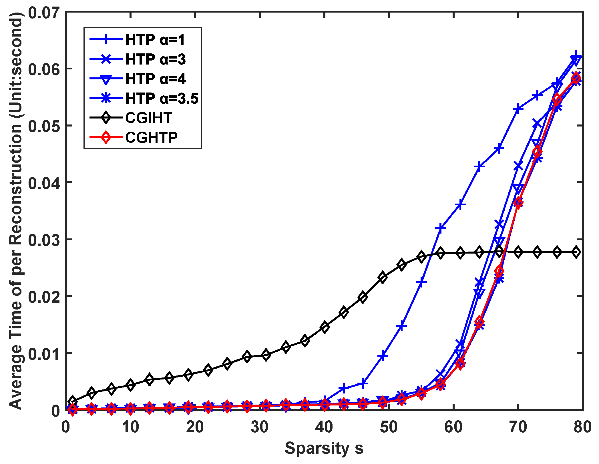
The first issue to be verified concerns the number of iterations required by the CGHTP algorithm in comparison with HTP algorithm and CGIHT algorithm. Here we choose the sampling rate . For each , we compute the average number of iterations of different algorithms and plot the curve in Figure 4, where we discriminated between successful reconstructions (mostly occurring for ) and unsuccessful reconstructions (mostly occurring for ). As can be seen from Figure 4, in the successful case, the CGHTP algorithm requires fewer iterations than the CGIHT algorithm and HTP algorithm with (in the case ). In the unsuccessful case, the number of iterations of CGHTP algorithm is comparable to that of HTP algorithm with . This is because for the same measurement matrix , when the sparsity level is small, the space formed by the columns of the is less correlated, so the condition number of is small, the advantage of using CG method is obvious; as the sparsity level increase, the condition number of becomes larger, which has a bad influence on the convergence rate of CGHTP. The average time consumed by different algorithms is shown in Figure 5. It can be seen that CGHTP algorithm requires the least average reconstruction time than other algorithms, because it requires fewer iterations than other algorithms.
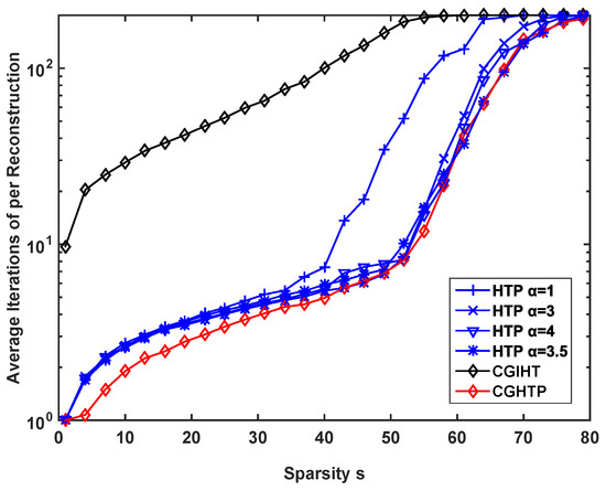
Figure 4.
Number of iterations for HTP with different step size, CGIHT, and CGHTP algorithms.

Figure 5.
Time consumed by HTP with different step size, CGIHT, and CGHTP algorithms.
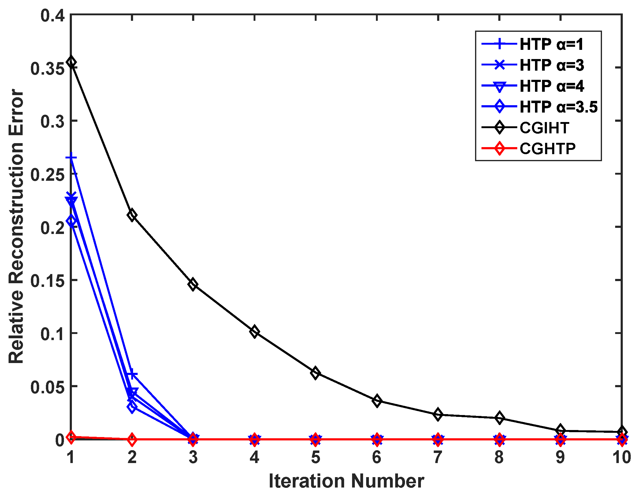
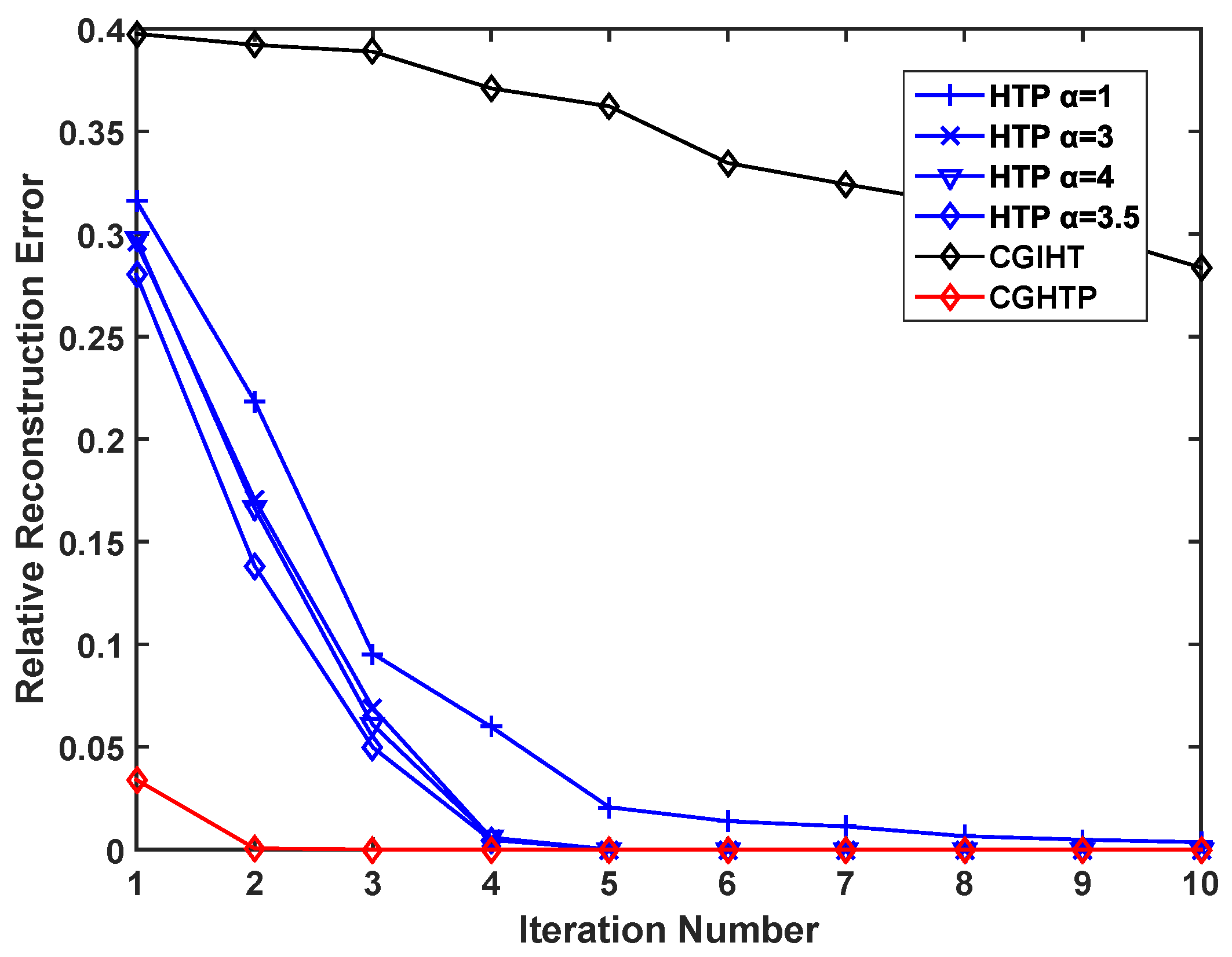
At the same time, to verify the advantages of the proposed algorithm in convergence speed, we select a fixed sparse signal and record the relative reconstruction errors of different algorithms under different number of iterations. As can be seen from Figure 6 and Figure 7, as the number of iterations increases, the relative reconstruction errors of the signals reconstructed by HTP and CGHTP decrease, and becomes stable at a certain error value where the convergence is reached. However, the relative reconstruction error of CGIHT algorithm decreases very slowly with the increase of iteration times. Figure 6 and Figure 7 show that the number of iterations for convergence of CGHTP algorithm is smaller than that of HTP algorithm with an optimal step size and CGIHT algorithm, which reflects that CGHTP algorithm converges faster than HTP algorithm and CGIHT algorithm. The acceleration strategy chosen by the gradient descent method and the conjugate gradient method results in a better performance of the CGHTP algorithm in convergence rate.
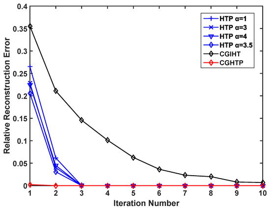
Figure 6.
Relative reconstruction error vs. iteration number, ().
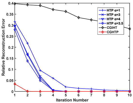
Figure 7.
Relative reconstruction error vs. iteration number, ().
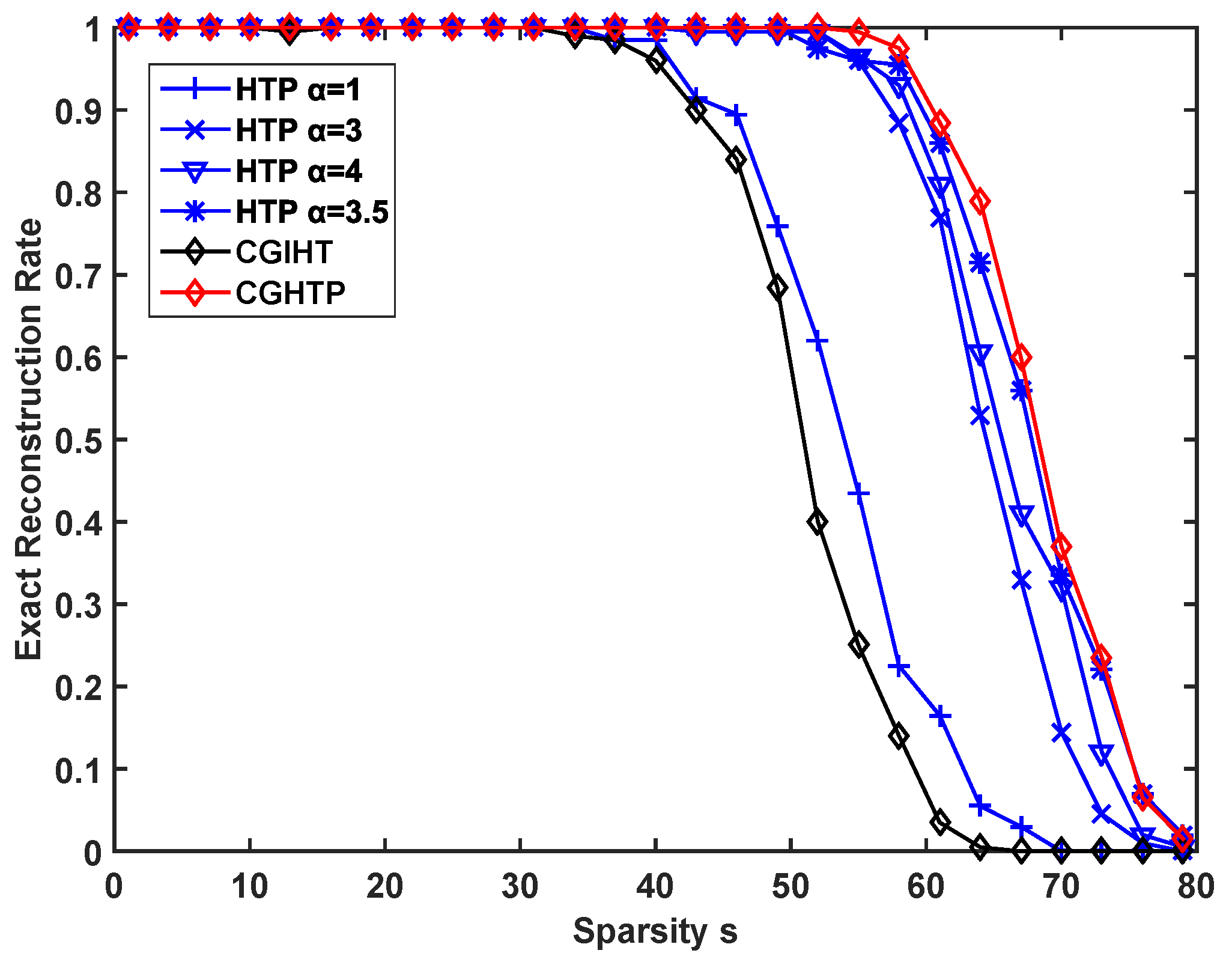
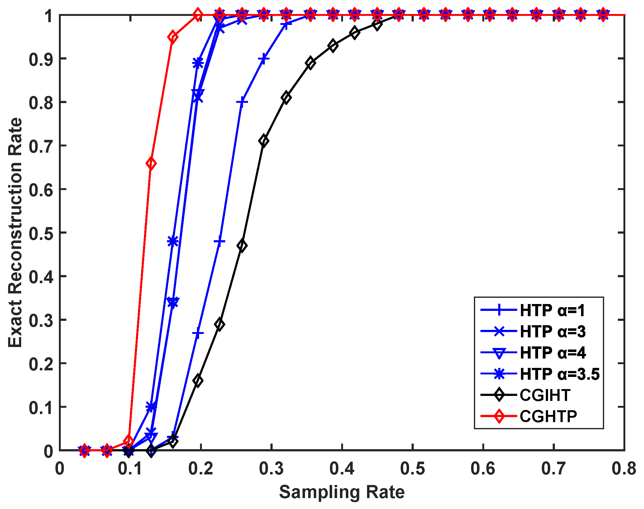
The recovery ability of the proposed algorithm is evaluated for different sparsity levels and different sampling rates. In each experiment, it is recorded as a successful reconstruction if . Figure 8 describes the exact reconstruction rate of different algorithms with different sparsity levels at a fixed sampling rate of while Figure 9 depicts the recovery performance of these algorithms at different sampling rates at a fixed sparsity level . Figure 8 and Figure 9 show that the CGHTP is outperforms other algorithms. In addition, for the same rate of exact reconstruction, CGHTP requires fewer samples than other algorithms.
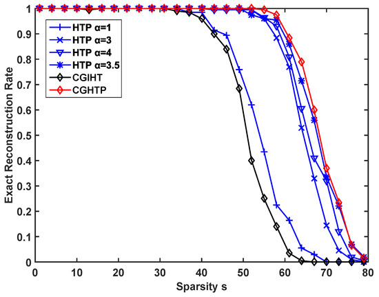
Figure 8.
Exact reconstruction rate vs. sparsity level for a Gaussian signal.
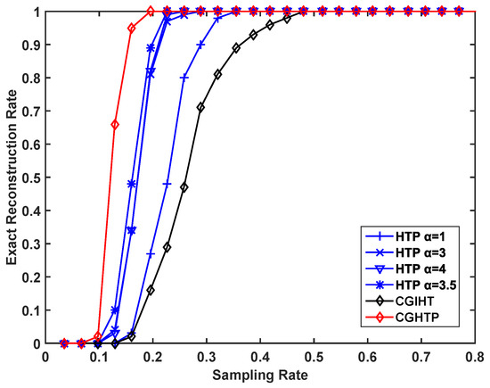
Figure 9.
Exact reconstruction rate vs. sampling rate for a Gaussian signal.
5.2. Real-World Image Reconstruction
In this subsection, we investigated the performance of CGHTP to reconstruct natural images. Test images used in experiments consist of four natural images of size 512 × 512, as shown in Figure 10a, Figure 11a, Figure 12a and Figure 13a respectively. We choose the discrete wavelet transform(DWT) matrix as the sparse transform basis and the Gaussian random matrix as the measurement matrix. The sparsity level is set to one sixth of the number of samples, i.e., . In all tests, each experiment is repeated 50 times independently and we set an algorithm-stopping criterion: or . The reconstruction performance of images is usually evaluated by the Peak Signal to Noise Ratio (PSNR), which is defined as:
where MSE denotes the mean square error, and it can be calculated by:
where the matrices and of size represent the original image and the reconstructed image. Meanwhile, we also consider using relative error (abbreviated as Rerr) to evaluate the quality of image reconstruction:
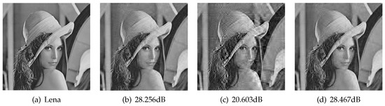
Figure 10.
The reconstruction results of the standard test image Lenna at . (a) original image; (b) reconstructed by HTP with , (PSNR: 28.256 dB); (c) reconstructed by CGIHT (PSNR: 20.603 dB); (d) reconstructed by CGHTP (PSNR: 28.467 dB).

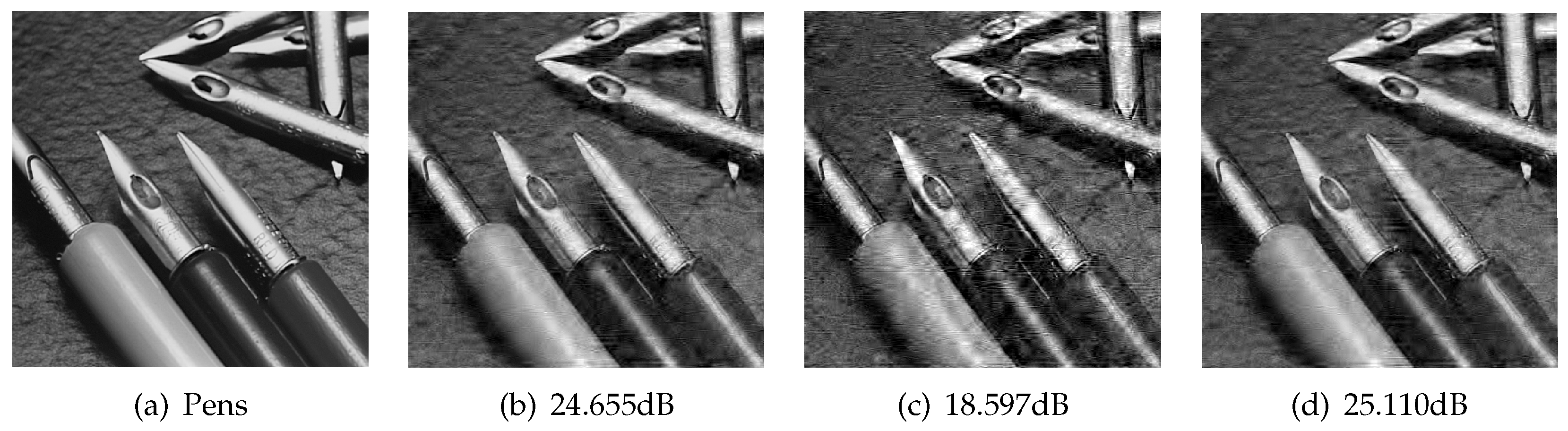
Figure 11.
The reconstruction results of the standard test image Pens at . (a) original image; (b) reconstructed by HTP with , (PSNR: 24.655 dB); (c) reconstructed by CGIHT (PSNR: 18.597 dB); (d) reconstructed by CGHTP (PSNR: 25.110 dB).
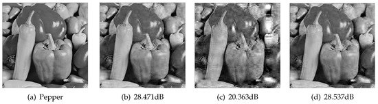
Figure 12.
The reconstruction results of the standard test image Pepper at . (a) original image; (b) reconstructed by HTP with , (PSNR: 28.471 dB); (c) reconstructed by CGIHT (PSNR: 20.363 dB); (d) reconstructed by CGHTP (PSNR: 28.537 dB).
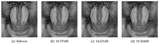
Figure 13.
The reconstruction results of the standard test image Baboon at . (a) original image; (b) reconstructed by HTP with , (PSNR: 18.333 dB); (c) reconstructed by CGIHT (PSNR: 14.621 dB); (d) reconstructed by CGHTP (PSNR: 18.364 dB).
Table 1 shows the average reconstruction PSNR, Rerr, and reconstruction time of four reconstructed images by different algorithms at different sampling rates. Figure 9, Figure 10, Figure 11 and Figure 12 visually reflects the contrast between the original image and the reconstructed image, where subfigure (b–d) represents the reconstructed images obtained by HTP (), CGIHT, and CGHTP, respectively.

Table 1.
Reconstruction results of Lenna, Pens, Pepper, and Baboon images at different sampling rates by HTP, CGIHT, and CGHTP. The optimal step size for reconstructing Lenna, Pens, Pepper and Baboon images by HTP algorithm are , , and , respectively. The abbreviations PSNR and Rerr in the table represent the Peak Signal to Noise Ratio and relative reconstruction error of the reconstructed image, respectively.
It can be seen from Table 1 that the reconstruction performance of different algorithms is different for four tested images. In terms of reconstruction PSNR value, the lower the sampling rate, the more obvious the advantage of CGHTP algorithm over HTP algorithm and CGIHT algorithm. Especially in the case of low sampling rate (T = 0.2), the reconstructed PSNR value of the four tested images obtained by CGHTP algorithm is about 2 dB higher than that obtained by HTP algorithm with the best step size. Similarly, the reconstruction relative error of CGHTP is slightly lower than that of other algorithms. In addition, the average reconstruction time of CGHTP is comparable to that of HTP algorithm with an optimal step size. Due to the calculation of the step size and the orthogonal factor , the CGHTP algorithm requires slightly more computation than the HTP algorithm by approximately . However, in each iteration, the conjugate direction may be used as the search direction in CGHTP to accelerate the convergence rate, so they need fewer iterations than the HTP algorithm. Overall, CGHTP has an empirical performance comparable to the HTP algorithm with an optimal step size in natural image reconstruction.
6. Conclusions
In this paper, we introduce a new greedy iterative algorithm, termed CGHTP. Using conjugate gradient method to accelerate the convergence of the original HTP algorithm is one of the strong features of the algorithm, which makes the CGHTP algorithm faster than the HTP algorithm. Reconstruction experiments with Gaussian sparse signals and natural images illustrate the advantages of the proposed algorithm in convergence rate and reconstruction performance, especially in the case of low sparsity, CGHTP requires fewer iterations than HTP with the best step size and CGIHT algorithm. Although the proposed algorithm has better reconstruction performance, its theoretical guarantee is not very strong, our future works may focus on the research about stronger theoretical guarantee of this algorithm. In addition, we will study how to apply this method to more practical applications.
Author Contributions
Conceptualization, Y.Z.; Data curation, Y.Z. and X.F.; Funding acquisition, Y.H.; Methodology, Y.Z.; Project administration, H.L.; Software, P.L. and X.F.; Validation, H.L., Y.H., P.L. and X.F.; Writing—original draft, Y.Z.; Writing—review & editing, Y.Z. and H.L.
Funding
This work was funded by National Natural Science Foundation of China under Grant Nos. 51775116, and 51374987, and 51405177, NSAF U1430124.
Conflicts of Interest
The authors declare no conflict of interest.
References
- Donoho, D.L. Compressed sensing. IEEE Trans. Inf. Theory 2006, 4, 1289–1306. [Google Scholar] [CrossRef]
- Eldar, Y.; Kutinyok, G. Compressed Sensing: Theory and Application; Cambridge University Press: Cambridge, UK, 2011; Volume 4, pp. 1289–1306. [Google Scholar] [CrossRef]
- Zhang, J.; Xiang, Q.; Yin, Y.; Chen, C.; Xin, L. Adaptive compressed sensing for wireless image sensor networks. Multimed. Tools Appl. 2017, 3, 4227–4242. [Google Scholar] [CrossRef]
- Chen, Z.; Fu, Y.; Xiang, Y.; Rong, R. A novel iterative shrinkage algorithm for CS-MRI via adaptive regularization. IEEE Signal Process. Lett. 2017, 10, 1443–1447. [Google Scholar] [CrossRef]
- Bu, H.; Tao, R.; Bai, X.; Zhao, J. A novel SAR imaging algorithm based on compressed sensing. IEEE Geosci. Remote Sens. Lett. 2015, 5, 1003–1007. [Google Scholar] [CrossRef]
- Craven, D.; McGinley, B.; Kilmartin, L.; Glavin, M.; Jones, E. Compressed sensing for bioelectric signals: A review. IEEE J. Biomed. Health Inform. 2015, 2, 529–540. [Google Scholar] [CrossRef] [PubMed]
- Candès, E.J.; Tao, T. Decoding by linear programming. IEEE Trans. Inf. Theory 2005, 12, 4203–4215. [Google Scholar] [CrossRef]
- Candès, E.J.; Romberg, J.; Tao, T. Robust uncertainty principles: Exact signal reconstruction from highly incomplete frequency information. IEEE Trans. Inf. Theory 2006, 2, 489–509. [Google Scholar] [CrossRef]
- Vujović, S.; Stanković, I.; Daković, M.; Stanković, L. Comparison of a gradient-based and LASSO (ISTA) algorithm for sparse signal reconstruction. In Proceedings of the 5th Mediterranean Conference on Embedded Computing, Bar, Montenegro, 12–16 June 2016; pp. 377–380. [Google Scholar] [CrossRef]
- Beck, A.; Teboulle, M. A fast iterative shrinkage-thresholding algorithm for linear inverse problems. SIAM J. Imaging Sci. 2009, 1, 183–202. [Google Scholar] [CrossRef]
- Xie, K.; He, Z.; Cichocki, A. Convergence analysis of the FOCUSS algorithm. IEEE Trans. Neural Netw. Learn. Syst 2015, 3, 601–613. [Google Scholar] [CrossRef]
- Zibetti, M.V.; Helou, E.S.; Pipa, D.R. Accelerating overrelaxed and monotone fast iterative shrinkage-thresholding algorithms with line search for sparse reconstructions. IEEE Trans. Image Process. 2017, 7, 3569–3578. [Google Scholar] [CrossRef]
- Cui, A.; Peng, J.; Li, H.; Wen, M.; Jia, J. Iterative thresholding algorithm based on non-convex method for modified ℓp-norm regularization minimization. J. Comput. Appl. Math. 2019, 347, 173–180. [Google Scholar] [CrossRef]
- Fei, W.; Liu, P.; Liu, Y.; Qiu, R.C.; Yu, W. Robust sparse recovery for compressive sensing in impulsive noise using p-norm model fitting. In Proceedings of the IEEE International Conference on Acoustics, Acoustics, Speech and Signal Processing (ICASSP), Shanghai, China, 20–25 March 2016. [Google Scholar] [CrossRef]
- Ghayem, F.; Sadeghi, M.; Babaie-Zadeh, M.; Chatterjee, S.; Skoglund, M.; Jutten, C. Sparse signal recovery using iterative proximal projection. IEEE Trans. Signal Process. 2018, 4, 879–894. [Google Scholar] [CrossRef]
- Dirksen, S.; Lecué, G.; Rauhut, H. On the gap between restricted isometry properties and sparse recovery conditions. IEEE Trans. Inf. Theory 2018, 8, 5478–5487. [Google Scholar] [CrossRef]
- Cohen, A.; Dahmen, W.; DeVore, R. Orthogonal matching pursuit under the restricted isometry property. Constr. Approx. 2017, 1, 113–127. [Google Scholar] [CrossRef]
- Satpathi, S.; Chakraborty, M. On the number of iterations for convergence of cosamp and subspace pursuit algorithms. Appl. Comput. Harmon. Anal. 2017, 3, 568–576. [Google Scholar] [CrossRef]
- Needell, D.; Vershynin, R. Signal recovery from incomplete and inaccurate measurements via regularized orthogonal matching pursuit. IEEE J. Sel. Top. Signal Process. 2010, 2, 310–316. [Google Scholar] [CrossRef]
- Wang, J.; Kwon, S.; Li, P.; Shim, B. Recovery of sparse signals via generalized orthogonal matching pursuit: A new analysis. IEEE Trans. Signal Process. 2016, 4, 1076–1089. [Google Scholar] [CrossRef]
- Yao, S.; Wang, T.; Chong, Y.; Pan, S. Sparsity estimation based adaptive matching pursuit algorithm. Multimed. Tools Appl. 2018, 4, 4095–4112. [Google Scholar] [CrossRef]
- Saadat, S.A.; Safari, A.; Needell, D. Sparse Reconstruction of Regional Gravity Signal Based on Stabilized Orthogonal Matching Pursuit (SOMP). Pure Appl. Geophys. 2016, 6, 2087–2099. [Google Scholar] [CrossRef]
- Cui, Y.; Xu, W.; Tian, Y.; Lin, J. Perturbed block orthogonal matching pursuit. Electron. Lett. 2018, 22, 1300–1302. [Google Scholar] [CrossRef]
- Shalaby, W.A.; Saad, W.; Shokair, M.; Dessouky, M.I. Forward-backward hard thresholding algorithm for compressed sensing. In Proceedings of the 2017 34th National Radio Science Conference (NRSC), Alexandria, Egypt, 13–16 March 2017; pp. 142–151. [Google Scholar] [CrossRef]
- Blumensath, T. Accelerated iterative hard thresholding. Signal Process. 2012, 3, 752–756. [Google Scholar] [CrossRef]
- Blanchard, J.D.; Tanner, J.; Wei, K. Conjugate gradient iterative hard thresholding: Observed noise stability for compressed sensing. IEEE Trans. Signal Process. 2015, 2, 528–537. [Google Scholar] [CrossRef]
- Blanchard, J.D.; Tanner, J.; Wei, K. CGIHT: Conjugate gradient iterative hard thresholding for compressed sensing and matrix completion. Inf. Inference J. IMA 2015, 4, 289–327. [Google Scholar] [CrossRef]
- Foucart, S. Hard thresholding pursuit: An algorithm for compressive sensing. SIAM J. Numer. Anal. 2011, 6, 2543–2563. [Google Scholar] [CrossRef]
- Bouchot, J.L.; Foucart, S.; Hitczenko, P. Hard thresholding pursuit algorithms: Number of iterations. Appl. Comput. Harmon. Anal. 2016, 2, 412–435. [Google Scholar] [CrossRef]
- Li, H.; Fu, Y.; Zhang, Q.; Rong, R. A generalized hard thresholding pursuit algorithm. Circuits Syst. Signal Process. 2014, 4, 1313–1323. [Google Scholar] [CrossRef]
- Sun, T.; Jiang, H.; Cheng, L. Hard thresholding pursuit with continuation for ℓ0 regularized minimizations. Math. Meth. Appl. Sci. 2018, 16, 6195–6209. [Google Scholar] [CrossRef]
- Jain, P.; Tewari, A.; Dhillon, I.S. Partial hard thresholding. IEEE Trans. Inf. Theory 2017, 5, 3029–3038. [Google Scholar] [CrossRef]
- Song, C.B.; Xia, S.T.; Liu, X.J. Subspace thresholding pursuit: A reconstruction algorithm for compressed sensing. In Proceedings of the 2015 IEEE International Symposium on Information Theory (ISIT), Hong Kong, China, 14–19 June 2015. [Google Scholar] [CrossRef]
- Powell, M.J.D. Some convergence properties of the conjugate gradient method. Math. Program. 1976, 1, 42–49. [Google Scholar] [CrossRef]


© 2019 by the authors. Licensee MDPI, Basel, Switzerland. This article is an open access article distributed under the terms and conditions of the Creative Commons Attribution (CC BY) license (http://creativecommons.org/licenses/by/4.0/).