The combined tide-forecasting model presented in this paper was checked against the observed tide level data at the Bay Waveland Yacht Club port in the USA, obtained from the website of the National Oceanic and Atmospheric Administration. The harmonic constants of four tidal constituents of the Bay Waveland Yacht Club tidal station are shown in
Table 1. The tidal coefficient of the port is 10.767, indicating a diurnal tide-only one high and low tide each day. The tidal level of this port was predicted by the proposed model. The astronomical part of the tidal height was calculated via harmonic analysis, obtaining 720 tidal calculations at 1 h intervals over 30 consecutive days in November 2018. Meanwhile, the non-astronomical part of the water level variation was determined by the ARIMA-SVR model, wherein the training set was compiled from 744 prediction residual data of the astronomical tidal levels from GMT0000 on 1 October 1 2018 to GMT2300 on 31 October 2018, and 720 prediction residual data from GMT0000 on 1 November 2018 to GMT 2300 on 30 November 2018, which were used as the test set for verifying the prediction results. Finally, both parts of the tidal calculation results were superimposed to obtain the predicted tidal levels throughout November 2018.
3.2.3. Analysis of Prediction Results of Non-Astronomical Tide Level
The model parameters of the non-astronomical part were determined by the single-step ARIMA model. To determine the difference term
, the stationarity of the sequence must be determined by visual processing. To this end, the 744 nonlinear data throughout October 2018 were processed by the augmented Dickey–Fuller (ADF) stationarity test. The parameters are shown in
Table 2. Here, the p-value is the probability of significance test in statistics, which is different from the order of the autoregressive model
mentioned in Formula (8). The
t-statistics were below the critical values at the 1%, 5%, and 10% significance levels, and the p-values were close to 0, confirming that the tidal level sequence was a stationary sequence with
= 0 [
22]. To determine the factors
in the autoregressive term and
in the moving average term, the sequence was evaluated by an autocorrelation function and a partial autocorrelation function [
23], respectively. The evaluation results are shown in
Figure 9 and
Figure 10, respectively. In the partial autocorrelation function plot (
Figure 9), the sequence is mainly located in the confidence interval after the third order; i.e., it begins to truncate after the third order, and the autoregressive term
is thus 3. After establishing
, the independent variables of the sample set in the SVR model are set to the tide levels at times
, and the dependent variable is the tide level at time
.
As is evident in the autocorrelation plot (
Figure 8), the tidal level time series is tailing, and the moving average term
is 0. In summary, the sequence establishes the ARIMA
model. The prediction process for the non-astronomical tidal part is shown in
Figure 11.
To reduce the influence of the order of magnitude of the sample on the prediction accuracy, the data in the training and test sets were normalized to the interval (0,1), and the RBF was selected as the kernel function. The parameters (penalty factor
and kernel function parameter
) were optimized by the PSO algorithm. The group termination algebra was set to 200; the population number was set to 20; and the learning factors
and
were set to 1.5 and 17, respectively. The optimization results are shown in
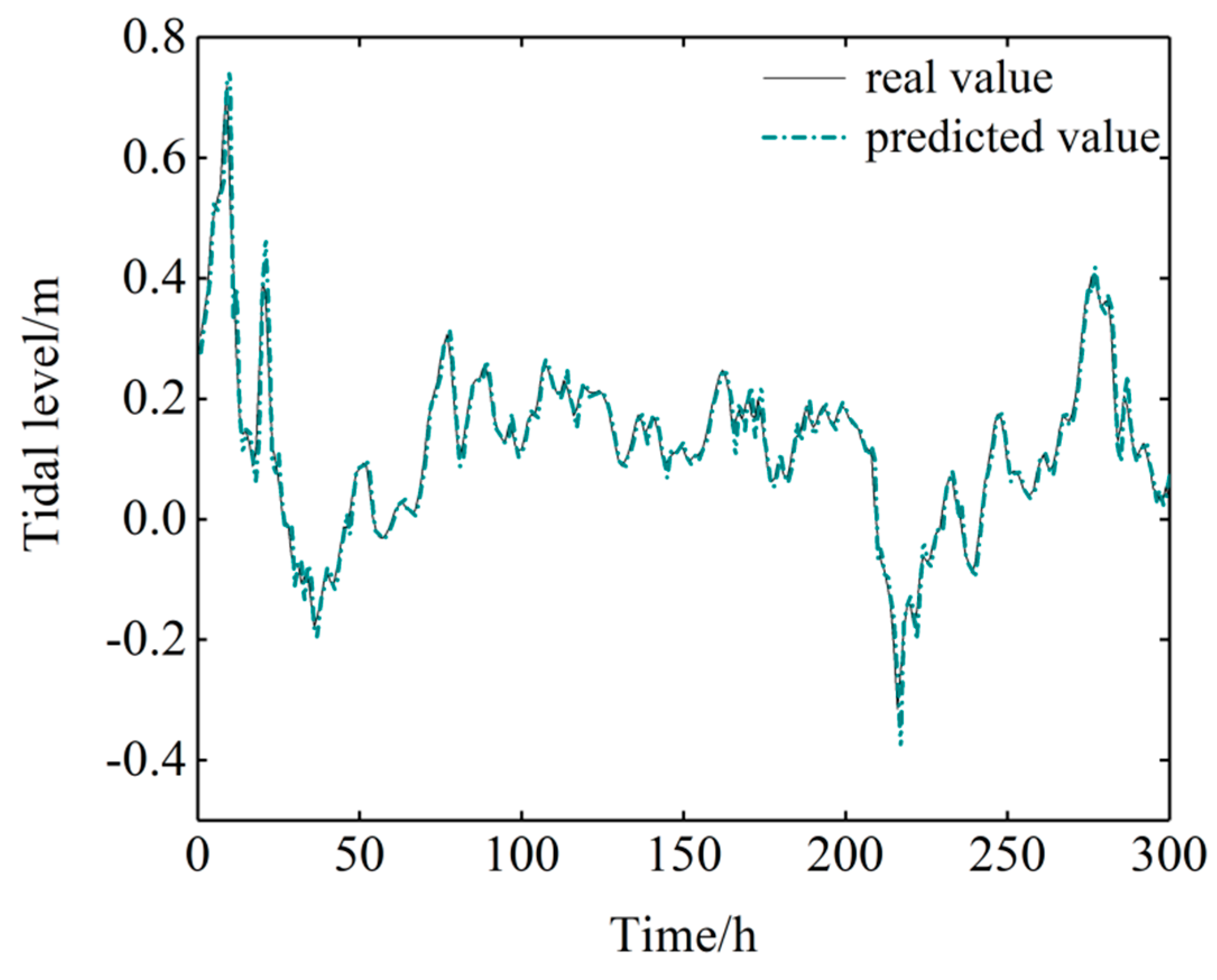
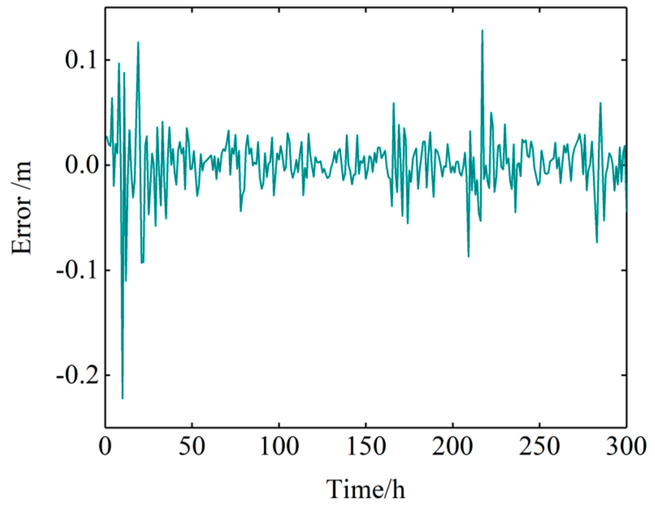
Table 3. The searched optimal parameters were input to the SVM model as the training data. After training, the test data were input to the model, and the predicted results were compared with the real results. The comparisons and their relative errors are displayed in
Figure 12 and
Figure 13, respectively.
3.2.4. Analysis of Prediction Results of the Combined Model
Next, the astronomical tidal level and the non-astronomical tidal level were linearly added to obtain the overall tidal prediction throughout November 2018.
Figure 14 compares the predicted tidal levels with the observed (not de-noised) data, and
Figure 15 plots the predicted errors. The combined model yielded much more accurate results than the pure harmonic analysis method. The
of the combined model was 0.022293 m, which is obviously smaller than that in the harmonic analysis method.
Figure 16 linearly regresses the predictions of the combined model against the observed (not de-noised) data. The combined model clearly predicted the observed tidal level with a high accuracy.
To verify the effect of de-noising, the tide level was predicted using the original data (without de-noising) and the predicted error was calculated by the above steps. The errors in the predictions are compared with those of the de-noised data in
Table 4. Clearly, the wavelet transform smoothed the data and improved the prediction accuracy. This result confirms the feasibility and effectiveness of de-noising the sample data prior to analysis.
To further verify the prediction accuracy of the combined model, the total tidal levels at the Bay Waveland Yacht Club station were predicted by single harmonic analysis, the combined model, the SVR model, and another common method called back propagation neural networks (the BP model) [
24]. The parameters of the SVR model were optimized by the PSO algorithm. For a fair comparison, the sample data and parameters were identical in all methods. The prediction performances of the four methods are compared in
Table 5. The proposed combined model required a longer training time, but yielded more accurate tidal predictions with lower errors than the other models.
The prediction accuracy of a model depends on the size of the training set. Accordingly, the prediction accuracies of the SVR and combined models were compared on training sets with different sample sizes (samples collected over 1, 3, 6, or 12 months). In this comparison, the test set remained fixed. ARIMA modeling is performed on the training sets of different sample sizes, and the lagged order of time series
is determined, and the input of the model is determined thereby. Again, the data were the tidal levels at the Bay Waveland Yacht Club tidal station. The prediction results of the SVR model and the combined model are shown in
Table 6 and
Table 7, respectively. As the sample size increased, the
of the tidal levels predicted by the SVR model (
Table 6) changed substantially around 0.049, whereas those of the combined model (
Table 7) fluctuated around 0.022 m. By contrast, the error indicators of tidal prediction were lower in the combined model than in the SVR model. The combined model thus exhibited a more accurate and stable prediction performance than the SVR model alone, within a significantly lower runtime than the SVR model. This result confirms the efficiency of the combined model.
As mentioned above, the Bay Waveland Yacht Club tidal station experiences a diurnal tide. To test the combined model on different tidal types and stations, the harmonic analysis, SVR, and combined models were trained on the tidal level data from four stations with different tidal types, and their predictive performances were evaluated in each case. Nawiliwili, The Battery, and Texas Point tidal stations were selected for tidal prediction comparison experiments, which have different tidal types. The ARIMA model was established for the tidal data of different tidal stations to determine the lagged rank of the time series
, so the input of the non-astronomical tidal part was determined. The error results are shown in
Table 8. At all four stations, the combined model outperformed the pure harmonic analysis and pure SVR models. In order to further measure the prediction accuracy, the relative magnitude of the astronomical tide and non-astronomical tide parts of the sample data of four tidal station was calculated, and the following
Table 8 was obtained. As shown in
Table 8 and
Table 9, it can be seen that the larger the relative magnitude of the astronomical tide, the higher the accuracy of the harmonic analysis. The harmonic analysis method is suitable for predicting tidal stations with a high relative magnitude of astronomical tides.
The input of the SVR also significantly affects the prediction accuracy of the combined models. To verify the robustness of the input of SVR in the combined model determined according to the lagged rank
of the residual sequence in the ARIMA model, the combined model was trained on the tide level data from the Bay Waveland Yacht Club tidal station, and its predictive performance was compared for different inputs. The prediction results are shown in
Table 10. Here, the first column lists “
”, which refers to the fact that when the prediction time step is 1, the residual values from
to
moment is used to predict the value at time
t. Increasing the
from 1 to 3 reduced the error in the combined model, but increasing the
further increased the error. The minimized error at
= 3 is consistent with the test results of the lagged rank
of the residual sequence in the ARIMA model. However, even at the largest
(
= 12 ), the error was lower in the combined model than in the harmonic analysis method. Therefore, the combined model is more accurate and more suitable for short-term tidal level prediction than the simple harmonic model.


