A New Method for Markovian Adaptation of the Non-Markovian Queueing System Using the Hidden Markov Model

Abstract

This manuscript starts with a detailed analysis of the current solution for the queueing system M/Er/1/∞. In the existing solution, Erlang’s service is caused by Poisson’s arrival process of groups, but not individual clients. The service of individual clients is still exponentially distributed, contrary to the declaration in Kendall’s notation. From the related theory of the Hidden Markov Model (HMM), for the advancement of queueing theory, the idea of “hidden Markov states” (HMS) was taken. In this paper, the basic principles of application of HMS have first been established. 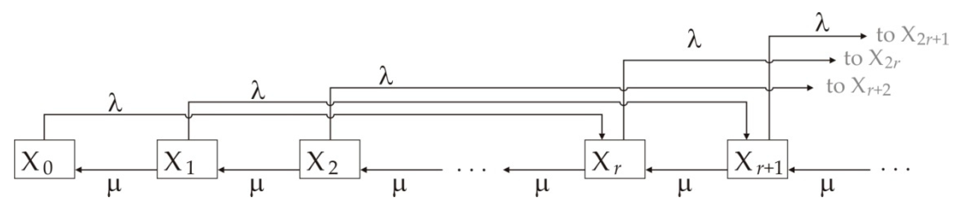The abstract HMS states have a catalytic role in the standard procedure of solving the non-Markovian queueing systems. The proposed solution based on HMS exceeds the problem of accessing identical client groups in the current solution of the M/Er/r queueing system. A detailed procedure for the new solution of the queueing system M/Er/1/∞ is implemented. Additionally, a new solution to the queueing system M/N/1/∞ with a normal service time N(μ, σ) based on HMS is also implemented.

1. Introduction

Queueing theory is a subfield of probability theory within mathematics. It was founded just over 100 years ago, by the publication of works and successful practical application of the Danish mathematician, statistician, and engineer Agner Krarup Erlang (1878–1929). In his honor, the system solved by M/M/1 and the unit of communication activity bears Erlang’s name. The effective practical application of the new queueing theory has given a strong impetus for it is further development. At the same time, the tasks posed by the practice require the solutions of non-Markovian and non-stationary queueing systems with a permanent imperative according to the standard set by Erlang—a transparent analytical solution.

The M/G/1 model was solved in 1930 by the Austrian-French engineer and mathematician, Félix Pollaczek (1892–1981) [1]. Our contemporary, Sir John Frank Charles Kingman, in 1961 [2], published an approximate formula for the mean waiting time in a G/G/1 queue. Although approximate, it is considered to be a very precise formula, especially for a system operating close to saturation. Of course, the most important contributions to the development of queueing theory must include contributions by David George Kendall (1918–2007) and another contemporary Jonh Dutton Conant Little (born 1928). The solutions of non-stationary queueing systems begin with the works by Andrey Nikolaevich Kolmogorov (1903–1987) [3], which emerged almost simultaneously with the first general solutions of the non-Markov queueing systems in 1930 [1].

Nevertheless, in spite of the great effort, intensive development of the world economy and the requirements of practice have far exceeded the achievements of queueing system researchers. The emergence and design of the development of computers in the 1980s and 1990s resulted in the prognosis that each queueing system could be solved by the use of simulations. This attitude has somewhat discouraged further efforts in the analytical approach of queueing theory and was consistently described by Koenigsberg in the set and reasoned antithesis [4]. His absolutely correct assessment of the necessity of an analytical approach and positive development prognosis was confirmed by Schwartz, Selinka, and Stoletz, especially for non-stationary time-dependent queueing systems [5]. The analytical approach to solving the queueing system remains an imperative. This imperative does not exist in itself, but is encouraged by the practical application of the queueing system.

The theory of the Hidden Markov Model (HMM) was founded by Baum and Petrie in the mid-1960s [6]. It is based on the simple idea that in the observed system, the Markov processes are a priori, and that the existence of hidden Markov states can be confirmed statistically, representing the criterion for optimizing the maximum probability. HMM is classified into methods of artificial intelligence. It is characterized by an intense development [7] and capacity for effectively solving a wide range of real tasks: character recognition [8], medicine [9], helping blind people [10], infrastructure management [11], driver fatigue detection [12], etc.

Basically, HMM is related to queueing theory. It also shares the same analytical problems in the principles of the functioning of a state in a non-Markovian domain [13]. The application of the idea of hidden states from HMM in queueing systems has an initially modest, but extremely important, realized methodological idea in the birth–death process [14].

The synthesis of HMM and queueing theory leads to the idea of abstract hidden states of Markov (HMS) in the first-order transition probability distribution among the hidden states with a possible catalytic function. This idea is not new, and HMS have already been developed for some higher-order Markov models [15]. For non-Markov queueing systems, the HMS function is contrary to convolution. It is based on the process of the decomposition of exponential random variables to the sum of exponential distributions. The exact case is Erlang’s distribution, which is a well-known relation presented in the following (1):

$$Er(k,\lambda )={\displaystyle \sum _{i=1}^{k}E(\lambda )}$$

(1)

The idea of the decomposition of Erlang’s distribution and reduction to the Markov queueing system was applied in the simplest case—the intensity of Erlang’s second-order distribution Er(2, μ), in the artificial intelligence hybrid known as Ant Colony Optimization [16].

In addition to Erlang’s distribution, we have at our disposal the relationship between an exponential distribution and normal distribution using the Central Limit Theorem [17].

2. Analysis of the Current Solution Queueing Systems M/E_r/1/∞ and E_k/E_r/1/∞

The recent solution of the M/E_k/r queueing system from 1968/69 [18,19] was based on the assumption that customers arrive at Poisson’s arrival process and are serviced by the Erlang distribution Er(k, µ). A well-known convolution was used to reduce the Markov queueing system (1). The analytical solution assumes the following flow diagram (Figure 1).

In this queueing system, the services of the Erlang distribution Er(k, μ) are realized through the “k” exponential E(μ) phases. The solution of the stationary state follows the set of equilibrium equations, which, along with the change p_n = xⁿ, requires the solution of the polynomial (2).

$$(\lambda +\mu )x^r=\lambda +\mu x^{r+1}$$

(2)

The roots of Equation (2) can be numerically determined very efficiently [20]. The solution of the queueing system E_k/E_r/1 had a similar problem which was also successfully mathematically solved in a similar way [21,22,23,24].

However, a comparative analysis of the mean number of customers in the simplest M/M/1/∞ and M/E_k/r/∞ systems leads us to a kind of paradox. Their relationship is as follows (3):

$$\underset{M/M/1/\infty }{\underbrace{\frac{\rho }{1-\rho }}}\le \underset{M/E_k/1/\infty }{\underbrace{\frac{{\rho }_k}{1-{\rho }_k}\cdot \frac{k+1}{2}}},(\mathrm{k}\ge 2)\in \mathrm{N};\frac{1}{\mu }=\frac{k}{{\mu }_k};\rho =\frac{\lambda }{\mu }={\rho }_k=\frac{k\lambda }{{\mu }_k}<1$$

(3)

Apparently, the current solution of M/E_k/r is “mechanically” configured to serve a group of “k” clients. If each client is served by the exponential distribution, a group of “k” clients will be served by the Erlang distribution. In practice, we have found this system in stochastic inventory management. At the same time intervals 1/λ, stocks are supplemented with the same quantity of “k” integer “customers” (Figure 2). The current solution of the M/E_k/r is not entirely adequate for the following reasons:

• Customers do not arrive at Poisson’s arrival process—a group of “k” customers arrive at Poisson’s arrival process. For this reason, the ratio of the number of clients in the queueing systems is (3);
• Customers are not served by Erlang’s distribution—customers are served by the exponential distribution. A group of “k” customers are served by Erlang’s distribution.

In recent solutions of the queueing system M/E_k/r, the state of the queue is redefined as the number of service stages remaining in the system [23]. Solutions of the first half of the century are still dominant [25], although these do not allow for successive transitions through the states of the system, as in the system M/M/1/∞. Simply, the queueing system M/E_k/r from Figure 1 does not have mutual transitions from neighboring states.

Paragraph (3) is not in agreement with the well-known Pollaczek–Khintchine formula. For the same mean service rate, the Erlang distribution has a lower value of variance than the exponential one. Therefore, the M/E_k/1/∞ system must have a smaller mean number of customers in the queue. The reason for this relationship is found in the projected flow diagram (Figure 1). Exponential phases of customer services through which the Erlang distribution is convoluted are partially realized, depending on the quantity λ and μ. For the interval 0 < ρ < 1, for small values, ρ → 0 solutions are satisfactory, but when ρ → 1, there are large deviations. When dynamically observed, the higher arrival rate λ, the earlier the convolution of the exponential customer services is interrupted, and we obtain a service of the Erlang order, which is an average of less than k. Therefore, a valid solution is only approximate for favorable relationships λ and μ.

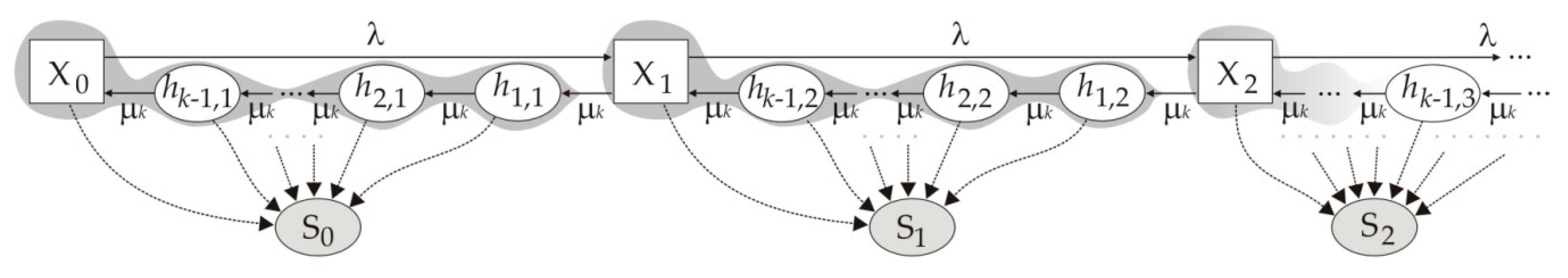
3. Analytical Solution of the Queueing System M(λ)/Ek(μ)/1/∞

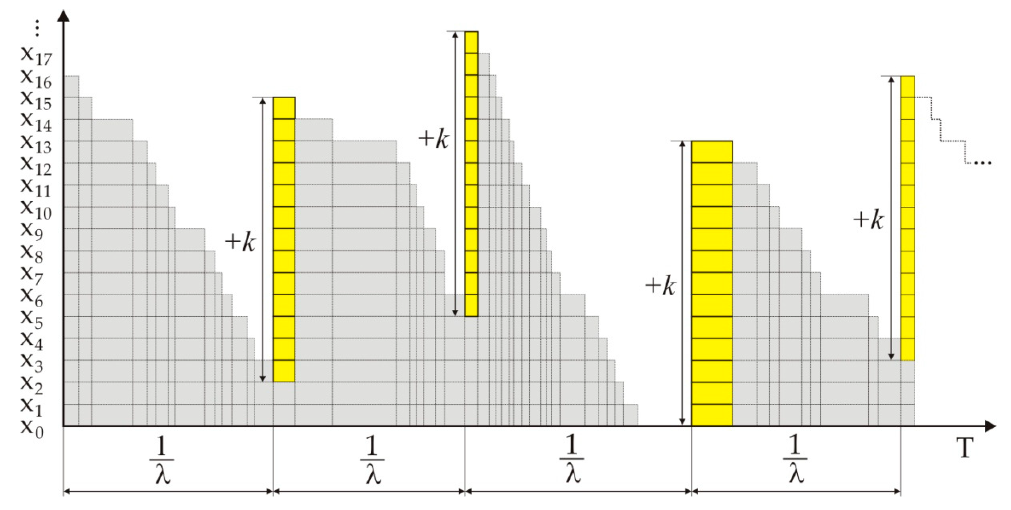
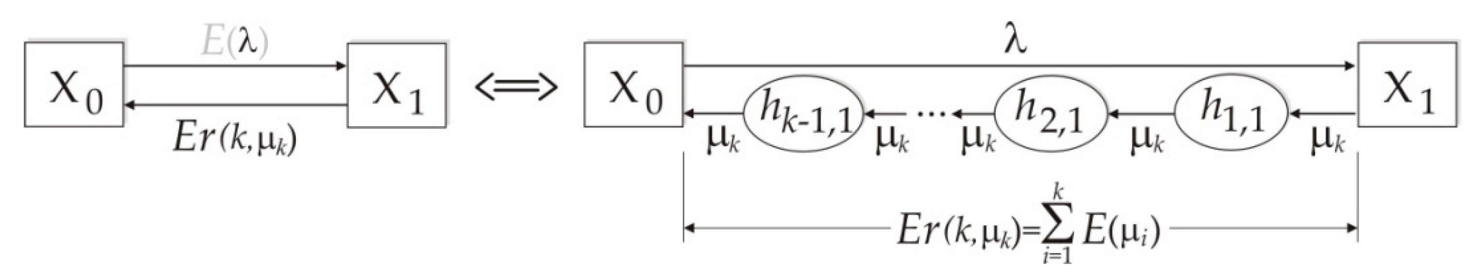
3.1. Elementary Case of Poison’s Birth and Erlang’s Death

The elementary case of the queueing system is based on the birth–death process. Therefore, consider the elementary system with two states X₀ and X₁. Let the time of birth be exponentially distributed E(λ) in this system, and the dying time be distributed according to Erlang’s distribution Er(k, μ_k).

Suppose that the birth–death process is ergodic and after a sufficiently long period, it achieves a stationary regime of operation with the following conditions: λ(t) = λ = const > 0, μ(t) = μ = const > 0, k ∈ N, k > 1.

This queueing system can be reduced to a Markov system by forming abstract hidden Markov states (HMS) based on the basic concept of HMM and the basic analytical description of the convolution of exponential distributions (1). The queueing system states h_k−1, h_k−2, …, h₂, h₁(k ∈ N) are abstract states and have a catalitic role. In order to achieve the convolution of “k” exponential distributions, the system needs to introduce “k − 1” abstract hidden Markov states in the process of customer services. The indexes of abstract states h_i are descendent. The symbolic equivalence of the birth–death process can be reduced to convincing by Markov with abstract, hidden states (Figure 3).

The solution of this system is based on the calculation of the probability values of all states: P(X₀) = p₀ and P(X₁) = p₁, as well as the probability of the state of abstract HMS h_k−1, h_k−2, …, h₂, h₁, respectively P(h_i) = p_h(i). We can calculate them with ease based on the existing analytical rules of the stationary regime of the birth–death process.

The key question is, how are the probabilities of abstract HMS p_h(i) classified? The existing system (Figure 2) has a “k + 1” state, and we only need two basic states: P₀ and P₁.

From the system of the birth–death process from two states, we know that in the first birth with intensity λ, the system goes into state X₁. Analogously, the intensity of dying μ_k from the beginning of the convolution translates the system into X₀ state, and the probability of abstract HMS is thus associated with the preceding state according to the following rule (4):

$$P_0=P(X_0)+P(h_{k-1})+\dots +P(h_1)=p_0+{\displaystyle \sum _{i=1}^{k-1}{p}_{h(1)}},P_1=P(X_1)=p_1$$

(4)

In the opposite case, when the birth time is distributed according to Erlang’s distribution Er (k, λ_k) and dying along the exponential E(μ), abstract HMS are formed for the purpose of convolution, but their probability will be added to the state P₁.

This describes the key catalytic principle of applying abstract HMS. The principle of grouping probabilities of basic and hidden states is given in Figure 4.

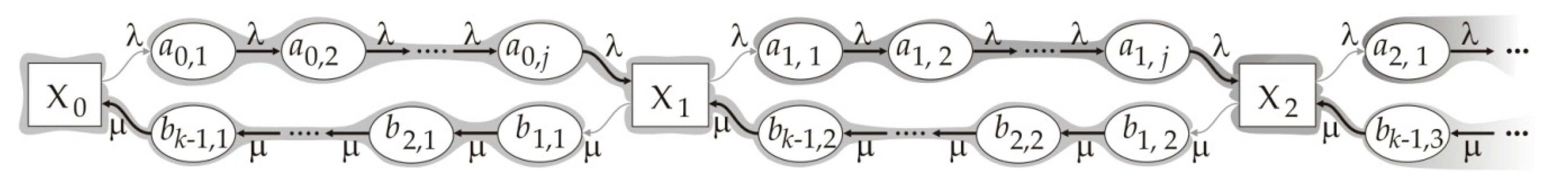
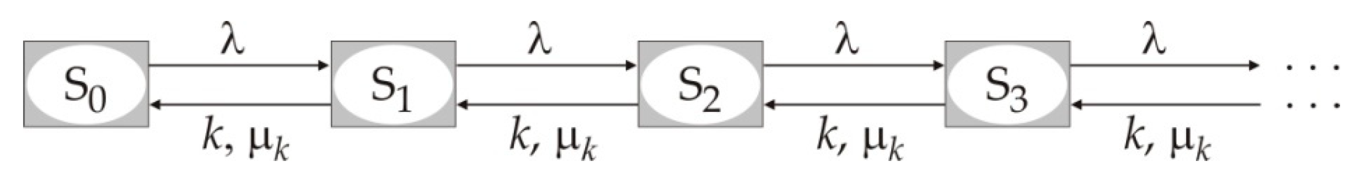
3.2. The Probability of State of the Queueing System M(λ)/E_k(μ)/∞

The establishment of the elementary case of a queueing system with a finite state number X₀, X₁, …, X_n, with the exponentially distributed inter-arrival-time E(λ) and the service time distributed according to Erlang’s distribution Er(k, μ_k), k ∈ N, is shown in Figure 5.

Assume that the queueing system is ergodic and that it is in a stationary operating mode. The probabilities of the state X₀, X₁, …, X_n, in the stationary mode of operation, are denoted by the large letter P_i(t) = P_i = const, i ∈ [1, n]. The probabilities of the abstract states h_i,j are denoted by the small letter p_i,j(t) = p_i,j = const, i ∈ [1, k−1], j ∈ [1, n]. For the X₀ state, the balance (differential) equation of the stady-state (stationary operating mode) is (5)

$$X_0:0=-\lambda P_0+{\mu }_k{p}_{k-1,1}\iff p_{k-1,1}=\frac{\lambda }{{\mu }_k}{P}_0$$

(5)

For the abstract HMS h_k−1,1, h_k−2,1, …, h_2,1, h_1,1 which are between the states X₀ and X₁, the system of balance equations of the stady-state is (6)

$$\{\begin{array}{l}{h}_{k-1,1}:0=-{\mu }_k{p}_{k-1,1}+{\mu }_k{p}_{k-2,1}\iff p_{k-1,1}=p_{k-2,1}\iff p_{k-2,1}=\frac{\lambda }{{\mu }_k}{P}_0\\ \dots \\ h_{2,1}:0=-{\mu }_k{p}_{2,1}+{\mu }_k{p}_{1,1}\iff p_{2,1}=p_{1,1}\iff p_{1,1}=\frac{\lambda }{{\mu }_k}{P}_0\\ h_{1,1}:0=-{\mu }_k{p}_{1,1}+{\mu }_k{P}_1\iff p_{1,1}=P_1\iff P_1=\frac{\lambda }{{\mu }_k}{P}_0\end{array}$$

(6)

For the state of X₁, the balance equation of the stady-state is (7)

$$X_1:0=\lambda P_0-\lambda P_1-{\mu }_k{P}_1+{\mu }_k{p}_{k-1,2}\iff p_{k-1,2}=\frac{-\lambda P_0+\lambda P_1+{\mu }_k{P}_1}{{\mu }_k}\iff p_{k-1,2}={\left(\frac{\lambda }{{\mu }_k}\right)}^2{P}_0$$

(7)

For the abstract HMS h_k−1,2, h_k−2,2, …, h_2,2, h_1,2 that are located between the states X₁ and X₂, the system of balance equations of the stady-state is (8)

$$\{\begin{array}{l}{h}_{k-1,2}:0=-{\mu }_k{p}_{k-1,2}+{\mu }_k{p}_{k-2,2}\iff p_{k-1,2}=p_{k-2,2}\iff p_{k-2,2}={\left(\frac{\lambda }{{\mu }_k}\right)}^2{P}_0\\ \dots \\ h_{2,2}:0=-{\mu }_k{p}_{2,2}+{\mu }_k{p}_{1,2}\iff p_{2,2}=p_{1,2}\iff p_{1,2}={\left(\frac{\lambda }{{\mu }_k}\right)}^2{P}_0\\ h_{1,2}:0=-{\mu }_k{p}_{1,2}+{\mu }_k{P}_2\iff p_{1,2}=P_2\iff P_2={\left(\frac{\lambda }{{\mu }_k}\right)}^2{P}_0\end{array}$$

(8)

For the state of X₂, the balance equation of the stady-state is (9)

$$X_2:0=\lambda P_1-\lambda P_2-{\mu }_k{P}_2+{\mu }_k{p}_{k-2,2}\iff p_{k-1,2}=\frac{-\lambda P_1+\lambda P_2+{\mu }_k{P}_2}{{\mu }_k}\iff p_{k-1,3}={\left(\frac{\lambda }{{\mu }_k}\right)}^3{P}_0$$

(9)

Prescriptively, in accordance with the standard solution procedure, we can obtain solutions for all remaining system states (10):

$$\begin{array}{l}\dots \dots \dots \dots \dots \dots \dots \\ X_{n-1}:0=\lambda P_{n-2}-\lambda P_{n-1}-{\mu }_k{P}_{n-1}+{\mu }_k{p}_{n,2}\iff p_{k-1,n}={\left(\frac{\lambda }{{\mu }_k}\right)}^n{P}_0\\ \{\begin{array}{l}{h}_{k-1,n}:0=-{\mu }_k{p}_{k-1,n}+{\mu }_k{p}_{k-2,n}\iff p_{k-1,n}=p_{k-2,n}\iff p_{k-2,n}={\left(\frac{\lambda }{{\mu }_k}\right)}^n{P}_0\\ \dots \\ h_{2,n}:0=-{\mu }_k{p}_{2,n}+{\mu }_k{p}_{1,n}\iff p_{2,n}=p_{1,n}\iff p_{1,n}={\left(\frac{\lambda }{{\mu }_k}\right)}^n{P}_0\\ h_{1,n}:0=-{\mu }_k{p}_{1,n}+{\mu }_k{P}_n\iff p_{1,n}=P_n\iff P_n={\left(\frac{\lambda }{{\mu }_k}\right)}^n{P}_0\end{array}\\ \dots \end{array}$$

(10)

The probability value P₀ can be obtained from the normative Equation (11):

$$\underset{s_0=P_0{\displaystyle \sum _{j=1}^{k-1}{\left(\frac{\lambda }{{\mu }_k}\right)}^1}}{\underbrace{P_0+P_0{\displaystyle \sum _{j=1}^{k-1}\frac{\lambda }{{\mu }_k}}}}+\underset{s_1=P_0{\displaystyle \sum _{j=1}^k{\left(\frac{\lambda }{{\mu }_k}\right)}^2}}{\underbrace{\underset{P_1}{\underbrace{P_0\frac{\lambda }{{\mu }_k}}}+P_0{\displaystyle \sum _{j=1}^{k-1}{\left(\frac{\lambda }{{\mu }_k}\right)}^2}}}+\dots +\underset{s_n=P_0{\displaystyle \sum _{j=1}^k{\left(\frac{\lambda }{{\mu }_k}\right)}^n}}{\underbrace{\underset{P_n}{\underbrace{P_0{\left(\frac{\lambda }{{\mu }_k}\right)}^2}}+P_0{\displaystyle \sum _{j=1}^{k-1}{\left(\frac{\lambda }{{\mu }_k}\right)}^n}}}+\dots =1$$

(11)

By solving the sum in (11), we can obtain (12)

$$\underset{s_0}{\underbrace{P_0+(k-1)P_0\frac{\lambda }{{\mu }_k}}}+\underset{s_1}{\underbrace{P_0\frac{\lambda }{{\mu }_k}+(k-1)P_0{\left(\frac{\lambda }{{\mu }_k}\right)}^2}}+\dots +\underset{s_n}{\underbrace{P_0{\left(\frac{\lambda }{{\mu }_k}\right)}^n+(k-1)P_0{\left(\frac{\lambda }{{\mu }_k}\right)}^{n+1}}}+\dots =1$$

(12)

The following geometric order is obtained (13):

$$P_0+k{P}_0\frac{\lambda }{{\mu }_k}+k{P}_0{\left(\frac{\lambda }{{\mu }_k}\right)}^2+k{P}_0{\left(\frac{\lambda }{{\mu }_k}\right)}^3\dots =1$$

(13)

where the condition λ < μ_k gives the equation for the P₀ (14) calculation.

We introduce the tag $\frac{\lambda }{{\mu }_k}={\rho }_k$:

$$P_0+k{P}_0{\displaystyle \sum _{j=1}^{\infty }{\left(\frac{\lambda }{{\mu }_k}\right)}^j=}{P}_0+k{P}_0\left(\frac{1}{1-{\rho }_k}-1\right)=P_0\left(\frac{1-{\rho }_k+k{\rho }_k}{1-{\rho }_k}\right)=1$$

(14)

The probability value of P₀ is equal (15) to

$$P_0-k{P}_0+P_0\frac{k}{1-{\rho }_k}=1\iff P_0=\frac{1-{\rho }_k}{1-{\rho }_k+k{\rho }_k}$$

(15)

The probabilities h_k−1,j, h_k−2,j, …, h_2,j, h_1,j (j ∈ N) are abstract probabilities. The analytical process takes them to the catalytic at each transition from the state X_j to the state X_j−1, for j ∈ [1, ∞). Therefore, the probabilities of p_i,j states h_i,j are abstractly transmitted only for the realization of the service by Erlang’s distribution. Now, the new code of the sum of probabilities of real and abstract states S_i (Figure 6) can be marked:

This is the demanded system with the exponentially distributed inter-arrival-time E(λ) and the service time distributed according to Erlang’s distribution Er(k, μ_k). We temporarily observe the label “k, μ” with the note that the service rate is distributed by Erlang’s “k” order with the intensity “μ_k” (Figure 7):

The probabilities of the state P(S_i) = s_i can be given by (16)

$$s_i=\frac{1-{\rho }_k}{1-{\rho }_k+k{\rho }_k}\left({\rho }_k^i+(k-1){\rho }_k^{i+1}\right)={\rho }_k^i\frac{1-{\rho }_k}{1-{\rho }_k+k{\rho }_k}\left(1+k{\rho }_k-{\rho }_k\right)={\rho }_k^i\left(1-{\rho }_k\right)$$

(16)

3.3. Comparison of the System M(λ)/M(μ_e)/1/∞ and M(λ)/E_k(μ_k)/1/∞

Now assume that the two queueing systems M(λ)/M(μ)/1/∞ and M(λ)/E_k(μ_k)/1 have an identical arrival rate and equal mean service time. Then, this relationship can be expanded with “λ” (17), as follows:

$$\frac{1}{\mu }=\frac{k}{{\mu }_k}\iff \frac{\lambda }{\mu }=\frac{\lambda k}{{\mu }_k}$$

(17)

By adopting the adopted columns for ρ and ρ_k, it follows that (18)

$$\rho =k{\rho }_k^{}\iff \frac{\rho }{k}={\rho }_k^{}$$

(18)

From the relationship (18), a new relationship of the variance for the same mean time of service in the queueing systems M(λ)/M(μ)/1/∞ and M(λ)/E_k(μ_k)/1/∞ (19) can be obtained:

$$\frac{1}{\mu }=\frac{k}{{\mu }_k}\iff \frac{1}{{\mu }^2}>\frac{k}{{\mu }_k^2}$$

(19)

In accordance with the Pollaczek–Khinchine formula, the queueing system with Erlang’s distribution of service times must have a lower mean number of customers in the system and queue. Contrary to paragraph (3) for the existing solution, we prove this statement for the new solution of the queueing system M(λ)/E_k(μ_k)/1/∞.

First, we recall the formula for calculating the probability state of the system M(λ)/M(μ)/1/∞, ρ = λ/μ (20):

$$p_i={\rho }^i(1-\rho )$$

(20)

We note that the probability calculus formulas (20) are analogous to (16). On the basis of this analogy, from the familiar formulas of the system M(λ)/M(μ_e)/1/∞ with smoothness, we proceed to the formula of the system M(λ)/E_k(μ_k)/1/∞. Now, the mean number of customers in the system M(λ)/E_k(μ_k)/1/∞ and in the queue equals (21)

$$L_s={\displaystyle \sum _{i=0}^{\infty }i\cdot {\rho }_k^i}(1-{\rho }_k^{})=\frac{{\rho }_k^{}}{1-{\rho }_k^{}},L_q=\frac{{\rho }_k^2}{1-{\rho }_k^{}},$$

(21)

By substituting (19) with (21), we obtain the basis for comparing the mean number of customers in the system and queue, i.e., for k > 1 and ρ < 1, the mean number of customers in the system M(λ)/E_k(μ_k)/1/∞ is always lower than the mean number of customers in the system M(λ)/M(μ_e)/1/∞. The same applies to the mean number of customers in the queue (22):

$$L_s=\underset{M(\lambda {)/E}_k({\mu }_k)/1/\infty }{\underbrace{\frac{\frac{\rho }{k}}{1-\frac{\rho }{k}}=\frac{\rho }{k-\rho }}}<\underset{M(\lambda )/M({\mu }_e)/1/\infty }{\underbrace{\frac{\rho }{1-\rho }}};L_q=\frac{{\left(\frac{\rho }{k}\right)}^2}{1-\frac{\rho }{k}}=\frac{{\rho }^2}{k(k-\rho )}<\frac{{\rho }^2}{1-\rho }$$

(22)

Unlike the relation in the previous queueing system solution M(λ)/E_k(μ_k)/1/∞ (3), the solution with the abstract HMS (21) completely meets the logic of the Pollaczek–Khinchine formula.

Using the Pollaczek–Khinchine formula for the queueing system M(λ)/E_k(μ_k)/1/∞, we can verify the validity of the patterns (21) and the relation (22). Mean service time and variance are distributed according to Erlang’s distribution with known parameters of mathematical expectation and standard deviation k/μ_k and k/μ_k², respectively. The ratio ρ is “k” times greater than ρ_k (18). If in the Pollaczek–Khinchine formula we reduce the intensity and the variance, we obtain (23), which is identical to the form (22) obtained:

$$L_s=\frac{\rho }{k}+\frac{{\left(\frac{\rho }{k}\right)}^2+{\lambda }^2\frac{Var(s)}{k}}{2\left(1-\frac{\rho }{k}\right)}=\frac{\rho }{k}+\frac{{\left(\frac{\rho }{k}\right)}^2+\frac{{\lambda }^2}{k(k{\mu }^2)}}{2\left(1-\frac{\rho }{k}\right)}=\frac{\rho }{k}+\frac{{\left(\frac{\rho }{k}\right)}^2+\frac{{\rho }^2}{k^2}}{2\left(1-\frac{\rho }{k}\right)}=\frac{\rho }{k-\rho }$$

(23)

By applying the Little formula, it follows that, for the same mean service time (18) and the relationships obtained (22), on average, customers spend more time on the M(λ)/M(μ_e)/1/∞ system. The amount of time $\phi$ is the same (24), as follows:

$$\phi =\frac{\frac{\lambda \rho }{k-\rho }}{\frac{\lambda \rho }{1-\rho }}=\frac{1-\rho }{k-\rho }<1$$

(24)

The same logic is applied for the mean wait in the queue. The explanation of this relationship is based on the relationship between the entropy of the exponential and Erlang’s distribution. Among all continuous probability distributions with support [0, ∞), the exponential distribution has the largest entropy. Therefore, the Markov queueing systems M/M/n/∞ have the greatest disadvantage in terms of access and service, and the greatest burden is thus on the service channel. In this case, in general, entropy is inversely proportional to the degree of system organization.

4. Queueing System M(λ)/N(ω, σ)/1/∞

4.1. An Approximate Solution

For Erlang’s distribution E_k(k, μ_k) and a normal distribution N(ω, σ) with a probability density function (25),

$$f_k(t)=\frac{{\mu }_k^k{t}^{k-1}{e}^{-{\mu }_k^{}t}}{(k-1)!},f(t)=\frac{1}{\sigma \sqrt{2\pi }}{e}^{-\frac{{(t-\omega )}^2}{2{\sigma }^2}}$$

(25)

With a sufficiently large value of the Erlang distribution line, based on the Central Limit Theorem (CLT) of Lindeberg–Levy, we can establish the following relations (26):

$$\omega =\frac{k}{{\mu }_k}\iff {\mu }_k=\frac{k}{\omega },\sigma =\frac{\sqrt{k}}{{\mu }_k}\iff {\mu }_k=\frac{\sqrt{k}}{\sigma }$$

(26)

For negative values of k, μ_k, ω, and σ, from the expression (26), we can obtain a quadratic equation. The solution of this square equation by “k ≥ 1” is equal to (27) the following:

$${\mu }_k^2=\frac{k^2}{{\omega }^2}=\frac{k}{{\sigma }^2}\iff \frac{k^2}{{\omega }^2}-\frac{k}{{\sigma }^2}=0,k_{1,2}=\frac{\frac{1}{{\sigma }^2}\pm \sqrt{\frac{1}{{\sigma }^4}}}{\frac{2}{{\omega }^2}},k_1=0\wedge k_2=\frac{{\omega }^2}{{\sigma }^2}$$

(27)

We can only find the solution k₂. In the case of distributing the service time by the normal distribution N(ω, σ), which in the application of the queueing system does not have negative values f(t) ≥ 0, t ∈ (0, ∞), due to the known rule (ω − 3σ) > 0 (with probability p = 0.9996), or the minimum value of the parameter “k”, we can expect 9. Thanks to the relation (26), the non-Markov queueing system M(λ)/N(ω, σ)/1/∞ can be reduced to the Markov queueing system with Erlang’s distribution of service times M(λ)/E(ω²/σ²,ω/σ²)/1/∞.

However, this form of expressing the normal distribution over Erlang’s is approximate, because the quantity (28) is a rational positive number (ω²/σ²) ∈ R⁺, i.e., a parameter of the Erlang distribution “k” will often not be the positive integer, k $\notin$ N. For practical use, the substitution (28) is approximative:

$$\frac{{\omega }^2}{{\sigma }^2}\notin N,Er(\underset{k}{\underbrace{\frac{{\omega }^2}{{\sigma }^2}}},\underset{{\mu }_n}{\underbrace{\frac{\omega }{{\sigma }^2}}})\approx N(\omega ,\sigma ),$$

(28)

4.2. Calibration of the Solution for a Normal Service Time

For each value of the non-negative rational number k ∈ R⁺ of the Erlang distribution curve obtained on the basis of (28), we can determine the value of Δ using the integer finite. We recall that in the case of the normal distribution of the service time N(ω, σ), the value of the parameter k ≥ 9 (29):

$$k=\frac{{\omega }^2}{{\sigma }^2}\ge 9,k-int(k)=\Delta ,0<\Delta <1$$

(29)

If we remember the definitions of the rational number, i.e., a number that can always be represented by a split of two integers, the rational value of the Erlang distribution parameters k ∈ R⁺ can be represented by a fraction formed by two selected natural numbers (a, b) ∈ N, which are greater than zero. Let k′ = int(k) and k″ = int(k) + 1. It follows that (30)

$$k=\frac{a{k}^{\prime }+b{k}^{″}}{a+b}$$

(30)

After determining the natural numbers (a, b), it is necessary to solve two systems:

• The first Erlang system of order k′, i.e., queueing system M(λ)/E(k′, ω²/σ²)/1/∞. Let us denote its probability as s_i′;
• The second Erlang system of order k″, i.e., queueing system M(λ)/E(k″, ω²/σ²)/1/∞. Let us identify its probabilities with s_i″.

If n_i denotes the probability of the state of the system M(λ)/N(ω, σ)/1/∞, after calculating the numbers (a, b) ∈ N, the probabilities of the state n_i (31) can be calculated as follows:

$$n_i=\frac{a{s}_i^{\prime }+b{s}_i^{″}}{a+b}$$

(31)

It is clear that in the calibration, the elementary-normative condition (32) is fulfilled:

$${\displaystyle \sum _{i=0}^{\infty }{n}_i}={\displaystyle \sum _{i=0}^{\infty }\frac{a{s}_i^{\prime }+b{s}_i^{″}}{a+b}}=\frac{{\displaystyle \sum _{i=0}^{\infty }(a{s}_i^{\prime }+b{s}_i^{″})}}{a+b}=\frac{a{\displaystyle \sum _{i=0}^{\infty }{s}_i^{\prime }+b}{\displaystyle \sum _{i=0}^{\infty }{s}_i^{″}}}{a+b}=\frac{a+b}{a+b}=1$$

(32)

This means that with a high precision, we can calculate the probabilities of the system M(λ)/N(ω,σ)/1/∞.

Calculations of the normal distribution can be substituted for sufficiently large k values. The formula for calculating the mean number of customers in the system and the queue (20) can also be applied k ∈ R⁺ for the purpose of the compulsory adjustment of μ_n = ω/σ according to formulas (26) and (27).

5. Conclusions

The application of abstract HMS with a catalytic function opens up many new possibilities in the analytical approach to the solution of the non-Markov queueing system. The process of reducing the non-Markov queueing system to Markov queueing systems is general. It is based on known convolutions and relations between exponential distributions and related distributions: Hyperexponential, Weibull, Rayleigh, Laplace, Gamma, etc. The concept of application is elastic, and it is applicable to heterogeneous queueing systems and various disciplines of services, etc.

The solutions of the queueing system M(λ)/E_k(μ_k)/1/∞ and M(λ)/N(ω, σ)/1/∞ were intended to demonstrate the effectiveness of the new proposed HMS-based method. The correctness of the new method is confirmed by the Pollaczek–Khinchine formula.

Based on the established principles of applying the HMS and the procedure, queueing system solutions with n channels of services and a finite number of positions in the queue are easy to obtain: M(λ)/E_k(μ_k)/n/m and M(λ)/N(ω, σ)/n/m. The extension of the HMS application principle provides solutions with queueing systems E_i/E_j/m/n (i ≠ j) i, j ∈ N, and by applying calibration, all queueing systems with a normally distributed time are analytically available.

The reasoned idea and principles of applying HMS can easily be applied to time-dependent queueing systems.

References

- Pollaczek, F. Uebereine Aufgabe der Wahrscheinlichkeits theory. Math. Z. 1930, 32, 64–100. [Google Scholar] [CrossRef]
- Kingman, J.F.C. The single server queue in heavy traffic. Math. Proc. Camb. Philos. Soc. 1961, 57, 902–904. [Google Scholar] [CrossRef]
- Kolmogorov, A. Sur le problèmed’attente. MatematicheskiiSbornik 1931, 38, 101–106. (In French) [Google Scholar]
- Koenigsberg, E. Is queueing theory dead? Omega 1991, 19, 69–78. [Google Scholar] [CrossRef]
- Schwarz, J.A.; Selinka, G.; Stolletz, R. Performance analysis of time-dependent queueing systems: Survey and classification. Omega 2016, 63, 170–189. [Google Scholar] [CrossRef] [Green Version]
- Baum, L.; Petrie, T. Statistical Inference for Probabilistic Functions of Finite State Markov Chains. Ann. Math. Stat. 1966, 37, 1554–1563. [Google Scholar] [CrossRef]
- Li, Y. Hidden Markov models with states depending on observations. Pattern Recognit. Lett. 2005, 26, 977–984. [Google Scholar] [CrossRef]
- Chen, M.Y.; Kundu, A.; Zhou, J. Off-line handwritten word recognition using a hidden Markov model type stochastic network. IEEE Trans. Pattern Recognit. Mach. Intell. 1994, 16, 481–496. [Google Scholar] [CrossRef]
- Uğuz, H.; Kodaz, H. Classification of internal carotid artery Doppler signals using fuzzy discrete hidden Markov model. Expert Syst. Appl. 2011, 38, 7407–7414. [Google Scholar] [CrossRef]
- Gu, F.; Zhang, H.; Zhu, D. Blind separation of non-stationary sources using continuous density hidden Markov models. Digit. Signal Process. 2013, 23, 1549–1564. [Google Scholar] [CrossRef]
- Kobayashi, K.; Kaito, K.; Lethanh, N. A statistical deterioration forecasting method using hidden Markov model for infrastructure management. Transp. Res. Part B Methodol. 2012, 46, 544–561. [Google Scholar] [CrossRef] [Green Version]
- Rongrong, F.; Hong, W.; Wenbo, Z. Dynamic driver fatigue detection using hidden Markov model in real driving condition. Expert Syst. Appl. 2016, 63, 397–411. [Google Scholar]
- Holzmann, H.; Schwaiger, F. Testing for the number of states in hidden Markov models. Comput. Stat. Data Anal. 2016, 100, 318–330. [Google Scholar] [CrossRef]
- Fadiloglu, M.M.; Yeralanm, S. Models of production lines as quasi-birth-death processes. Math. Comput. Model. 2002, 35, 913–930. [Google Scholar] [CrossRef] [Green Version]
- Ching, W.K.; Huang, X.; Ng, M.K.; Siu, T.K. Hidden Markov Chains. In Markov Chains. International Series in Operations Research & Management Science; Mamon, R.S., Elliott, R.J., Eds.; Springer: Boston, MA, USA, 2013; Volume 189, pp. 201–230. [Google Scholar]
- Tanackov, I.; Stojić, G.; Tepić, J.; Kostelac, M.; Sinani, F.; Sremac, S. Golden Ratio (Sectiona Aurea) in Markovian Ants AI Hybrid. Adaptive and Intelligent Systems, ICAIS 2011, Lecture Notes in Computer Science; Springer: Berlin, Germany, 2011; Volume 6943, pp. 356–367. [Google Scholar]
- Whitt, W. A broad view of queueing theory through one issue. Queueing Syst. 2018, 89, 3–14. [Google Scholar] [CrossRef]
- Heffer, J.C. Steady-state solution of the M/Ek/c (0, FIFO) queueing system. INFOR J. Can. Oper. Res. Soc. 1969, 17, 16–30. [Google Scholar]
- Mayhugh, J.O.; Mc Cormick, R.E. Steady state solution of the queue M/Ek/r. Manag. Sci. 1968, 14, 692–712. [Google Scholar] [CrossRef]
- Poyntz, C.D.; Jackson, R.R.P. The steady-state solution for the queueing process Ek/Em/r. Oper. Res. Q. 1973, 24, 615–625. [Google Scholar] [CrossRef]
- Adan, I.; Zhao, Y. Analyzing GI/Er/1 queues. Oper. Res. Lett. 1996, 19, 183–190. [Google Scholar] [CrossRef]
- Adan, I.J.B.F.; Van de Waarsenburg, W.A.; Wessels, J. Analyzing Ek/E/c queues. Eur. J. Oper. Res. 1996, 92, 112–124. [Google Scholar] [CrossRef]
- Martínez, J.M.V.; Vallejos, R.A.C.; Barría, M.M. On the limiting probabilities of the M/Er/1 queueing system. Stat. Probab. Lett. 2014, 88, 56–61. [Google Scholar] [CrossRef]
- Wang, K.H.; Kuo, M.Y. Profit analysis of the M/Er/1 machine repair problem with a non-reliable service station. Comput. Ind. Eng. 1997, 32, 587–594. [Google Scholar] [CrossRef]
- Adan, I.; Resing, J. Queueing Systems; Einhoven University of Technology: Eindhoven, The Netherlands, 2015. [Google Scholar]
© 2019 by the authors. Licensee MDPI, Basel, Switzerland. This article is an open access article distributed under the terms and conditions of the Creative Commons Attribution (CC BY) license (http://creativecommons.org/licenses/by/4.0/).
Share and Cite
Tanackov, I.; Prentkovskis, O.; Jevtić, Ž.; Stojić, G.; Ercegovac, P. A New Method for Markovian Adaptation of the Non-Markovian Queueing System Using the Hidden Markov Model. Algorithms 2019, 12, 133. https://doi.org/10.3390/a12070133
Tanackov I, Prentkovskis O, Jevtić Ž, Stojić G, Ercegovac P. A New Method for Markovian Adaptation of the Non-Markovian Queueing System Using the Hidden Markov Model. Algorithms. 2019; 12(7):133. https://doi.org/10.3390/a12070133
Chicago/Turabian StyleTanackov, Ilija, Olegas Prentkovskis, Žarko Jevtić, Gordan Stojić, and Pamela Ercegovac. 2019. "A New Method for Markovian Adaptation of the Non-Markovian Queueing System Using the Hidden Markov Model" Algorithms 12, no. 7: 133. https://doi.org/10.3390/a12070133
APA StyleTanackov, I., Prentkovskis, O., Jevtić, Ž., Stojić, G., & Ercegovac, P. (2019). A New Method for Markovian Adaptation of the Non-Markovian Queueing System Using the Hidden Markov Model. Algorithms, 12(7), 133. https://doi.org/10.3390/a12070133