A Fast Randomized Algorithm for the Heterogeneous Vehicle Routing Problem with Simultaneous Pickup and Delivery

Abstract

In the vehicle routing problem with simultaneous pickup and delivery (VRPSPD), customers demanding both delivery and pickup operations have to be visited once by a single vehicle. In this work, we propose a fast randomized algorithm using a nearest neighbor strategy to tackle an extension of the VRPSPD in which the fleet of vehicles is heterogeneous. This variant is an NP-hard problem, which in practice makes it impossible to be solved to proven optimality for large instances. To evaluate the proposal, we use benchmark instances from the literature and compare our results to those obtained by a state-of-the-art algorithm. Our approach presents very competitive results, not only improving several of the known solutions, but also running in a shorter time.

1. Introduction

The vehicle routing problem with simultaneous pickup and delivery (VRPSPD) [1,2,3,4,5,6,7,8,9], in which customers demanding both delivery and pickup operations have to be visited once by a single vehicle, is one of the main classes of the vehicle routing problem (VRP). This class has attracted research attention due to its applicability in numerous reverse logistic systems. For instance, in the bottled drinks industry, full bottles are delivered and empty ones are collected simultaneously from the customers. In fact, companies are increasingly faced with the task of managing the reverse flow of finished goods or raw materials [6]. In this context, one should consider together the logistics of distribution and the management of the reverse flow to minimize pickup and delivery operational efforts. Originally, the VRPSPD assumes a homogeneous fleet of vehicles. However, in many practical situations, companies employ a heterogeneous fleet of vehicles to satisfy customer demands. In this paper, we focus our attention on this variant of the VRPSPD. In fact, the heterogeneous vehicle routing problem with simultaneous pickup and delivery (HVRPSPD) has received research interest only in very recent years [10,11,12,13].

The HVRPSPD can be formally stated as follows: Let $G=(\mathcal{N},\mathcal{A})$ be a complete directed graph with a set of nodes $\mathcal{N}=\{0,1,\dots ,n\}$, where the node 0 represents the central depot and the remaining nodes denote the customers. Each customer $i\in \mathcal{N}-\left\{0\right\}$ has non-negative delivery $d_i$ and pickup $p_i$ demands. Each arc $ij\in \mathcal{A}$ is associated with a distance $c_{ij}$ from node i to node j. The fleet of vehicles involves T different vehicle types, and there is no restriction on the number of vehicles of each type. Every vehicle type $t=1,2,\dots ,T$ is associated with a fixed cost $f_t$, a variable cost per distance unit $g_t$, and a capacity $q_t$. We aim to determine the fleet composition and the set of vehicle routes that minimize the total cost, such that each vehicle travels exactly one route; each route starts and ends at the depot; each customer is visited only once by one of the vehicles; the vehicle completely satisfies the pickup and delivery demands of the customers on its route; the load carried by a vehicle must not exceed its capacity.

This problem has mainly been tackled by means of metaheuristics. In [10], a hybrid heuristic based on simulated annealing and local search is proposed to solve medium and large-size instances of the HVRPSPD. In [11], the authors propose a multi-label-based ant colony system algorithm to address the HVRPSPD. An initial solution is obtained by a nearest neighbor strategy, and then the ant colony system algorithm is applied to minimize the total number of vehicles used to attend the customers and the total travel distance performed by the vehicles. To evaluate their algorithm, they use benchmark problem instances adapted from other classes of the VRP. In [12], the authors present a mathematical model for the problem and propose some valid inequalities. In addition, a hybrid matheuristic based on the mathematical formulation in conjunction with a local search is presented. The state-of-the-art approach to tackle the HVRPSPD, to the best of our knowledge, appears in [13]. The authors propose the integration of an adaptive threshold strategy into a tabu search algorithm to avoid getting trapped in local minima. Their approach is based on neighborhood search and defines four different neighborhood structures to explore the solution space. It employs a giant tour representation to encode solutions and a decoding mechanism to partition the giant tour into feasible vehicle routes. For each giant tour, a cost network representation is constructed and a Djikstra algorithm is used to provide an optimal partition of the customers. A set of randomly generated problem instances is used to testify to the potentialities of the approach, and the authors argue that it can produce effective solutions in reasonable computation times.

In this paper, we propose a fast randomized algorithm using a nearest neighbor strategy to tackle the HVRPSPD. We use the same instances from [13], and computational experiments show that our approach presents very competitive results especially for large instances, not only improving several of the best known solutions, but also running in a shorter time.

The remainder of this paper is organized as follows. In Section 2, we present a mixed integer linear programming (MILP) formulation to the HVRPSPD and propose our fast randomized algorithm for tackling this problem. In Section 3, we provide computational experiments on benchmark instances from the literature. In Section 4, we present a detailed discussion of the results. Finally, in Section 5, we close the paper with some conclusions and future perspectives.

2. Materials and Methods

In this section, we first reintroduce the MILP formulation for the HVRPSPD proposed in [13] and then propose our fast randomized algorithm for tackling the problem.

2.1. MILP Formulation

Let $N=\{1,2,\dots ,n\}$ be the set of all customers and $N_0=N\cup \left\{0\right\}$ be the set of all customers and the depot. For each customer $j\in N$, $d_j$ and $p_j$ denote, respectively, its delivery and the pickup amounts. The fleet of vehicles is denoted by $V=\{1,2,\dots ,m\}$. Note that for the sake of modeling simplicity, the number of vehicles available of each type is already given in this formulation. This assumption, however, limits the decision on the fleet composition, and commonly, a sufficiently high number of vehicles has to be assumed for each vehicle type such that optimality can be guaranteed. For each vehicle $k\in V$, $q^k$, $f^k$, and $g^k$ denote, respectively, its capacity, fixed cost, and variable cost. In addition, for each pair of nodes $i,j\in N_0$, $c_{ij}$ represents the distance between the nodes.

We aim to determine the fleet composition and vehicle routes that minimize the total routing cost. Let $x_{ij}^k$ be the binary decision variable indicating whether vehicle k traverses arc $ij$ or not. The continuous variable $y_{ij}^k$ denotes the total load picked up by vehicle k while traversing arc $ij$. Conversely, the continuous variable $z_{ij}^k$ denotes the total load to be delivered by vehicle k while traversing arc $ij$. The optimization problem can be formulated as follows.

$$\begin{array}{cc}\hfill min& \sum _{k\in V}\sum _{j\in N}{f}^k{x}_{0j}^k+\sum _{k\in V}\sum _{i\in N_0}\sum _{j\in N_0}{c}_{ij}{g}^k{x}_{ij}^k\hfill \end{array}$$

(1)

$$\begin{array}{ccc}\hfill \mathrm{s}.\mathrm{t}.& \sum _{k\in V}\sum _{i\in N_0}{x}_{ij}^k=1\hfill & \hfill \forall j\in N\end{array}$$

(2)

$$\begin{array}{cc}\sum _{i\in N_0}{x}_{iv}^k-\sum _{j\in N_0}{x}_{vj}^k=0\hfill & \hfill \forall v\in N_0,k\in V\end{array}$$

(3)

$$\begin{array}{cc}\sum _{j\in N}{x}_{0j}^k\le 1\hfill & \hfill \forall k\in V\end{array}$$

(4)

$$\begin{array}{cc}{y}_{0j}^k=0\hfill & \hfill \forall j\in N,k\in V\end{array}$$

(5)

$$\begin{array}{cc}{z}_{i0}^k=0\hfill & \hfill \forall i\in N,k\in V\end{array}$$

(6)

$$\begin{array}{cc}\sum _{j\in N_0}\sum _{k\in V}{y}_{vj}^k-\sum _{i\in N_0}\sum _{k\in V}{y}_{iv}^k=p_v\hfill & \hfill \forall v\in N\end{array}$$

(7)

$$\begin{array}{cc}\sum _{i\in N_0}\sum _{k\in V}{z}_{iv}^k-\sum _{j\in N_0}\sum _{k\in V}{z}_{vj}^k=d_v\hfill & \hfill \forall v\in N\end{array}$$

(8)

$$\begin{array}{cc}\sum _{i\in N}\sum _{k\in V}{y}_{i0}^k=\sum _{v\in N}{p}_v\hfill & \hfill \end{array}$$

(9)

$$\begin{array}{cc}\sum _{j\in N}\sum _{k\in V}{z}_{0j}^k=\sum _{v\in N}{d}_v\hfill & \hfill \end{array}$$

(10)

$$\begin{array}{cc}{y}_{ij}^k+z_{ij}^k\le q^k{x}_{ij}^k\hfill & \hfill \forall i\in N_0,j\in N_0,k\in V\end{array}$$

(11)

$$\begin{array}{cc}{x}_{ij}^k\in \{0,1\},y_{ij}^k\ge 0,z_{ij}^k\ge 0\hfill & \hfill \forall i\in N_0,j\in N_0,k\in V\end{array}$$

(12)

The objective function (1) minimizes the total fixed costs of vehicles and variable transportation costs. Constraints (2) guarantee that each customer is visited exactly once. Constraints (3) impose the condition that each customer is served by the same vehicle. Constraints (4) ensure that each vehicle can serve one route at most. Constraints (5) guarantee that there is no demand picked up in the beginning of routes. Conversely, constraints (6) impose the condition that there is no demand for delivery in the end of routes. Constraints (7) and (8) are flow equations for pickup and delivery loads, respectively. Constraints (9) and (10), respectively guarantee that the sum of the inflow to the origin is equal to the total pickup demand and that the sum of the outflow from the origin is equal to the total delivery demand. Constraints (11) ensure that the capacity of the vehicles is respected throughout the routes. Finally, constraints (12) specify the domain of variables. The MILP model (1)–(12) contains $O\left(m{n}^2\right)$ binary variables and $O\left(mn\right)$ constraints.

2.2. Nearest-Neighbor-Based Randomized Algorithm

The original nearest neighbor algorithm is perhaps the simplest heuristic for the traveling salesman problem (TSP) [14], which is a classical optimization problem closely related to the VRP. The key to this algorithm is to always visit the nearest unvisited city (customer). It is well known that the nearest neighbor algorithm, a popular choice for tour construction heuristics, works at an acceptable level for the Euclidean TSP, but it can produce very poor results for the general TSP [15,16].

We now introduce our nearest-neighbor-based randomized algorithm to tackle the HVRPSPD, as shown in Algorithm 1. In our approach, at each iteration of the main loop of the algorithm (line 2), a feasible solution to the HVRPSPD (i.e., a set of feasible routes, each of them associated with a vehicle type, to cover all customers) is constructed from scratch. We keep track of the best solution obtained during iterations, but it is not used to define a neighborhood structure or to guide the search for better solutions and, in this respect, it can be seen as a blind search. The construction of a feasible solution, however, is probabilistically guided by two alternative greedy criteria to select the next customer to be visited on the current route: the nearest neighbor or the first one from a given list of unvisited customers. In the sequel, we explain the construction of a feasible solution in more detail.

Algorithm 1: Nearest-Neighbor-Based Randomized Algorithm

parameters: Computation time limit $\tau$, probability  $\rho$ of using the nearest neighbour strategy. input: Set of $customers$ and $depot$, set of vehicle $types$. output: Set of vehicle routes ($bestRoutes$).

At each iteration, to obtain a feasible solution, we first generate a random permutation of all customers. We maintain a list of customers that were not served by a vehicle yet, named as $unvisitedCustomers$, which is initially set with the random permutation. The routes of a feasible solution are generated sequentially. For each route, we randomly choose a vehicle among all types. The route always starts from the depot to the first customer from $unvisitedCustomers$ whose delivery and pickup demands respect the capacity of the vehicle used to serve the route. Thereafter, the next customer under consideration to be appended to the route, named as $trial$, is chosen either by the ordering of $unvisitedCustomers$ or by the nearest neighbor strategy, according to a probability $\rho$. Every time $trial$ has been effectively added to the current route, it is removed from $unvisitedCustomers$. And every time $trial$ has been proven to be infeasible to be part of the route (because of a vehicle capacity violation), we set its property $infeasible=\mathsf{true}$, and then it is no more considered to be part of this route. The algorithm follows this process until there are no more customers that can be appended to the current route. In this case, the current route is closed, the feasibility of customers in $unvisitedCustomers$ is reestablished ($infeasible=\mathsf{false}$), and a new route is opened. Routes are created until all customers have been visited ($unvisitedCustomers$ is empty), when we obtain a feasible solution to the HVRPSPD.

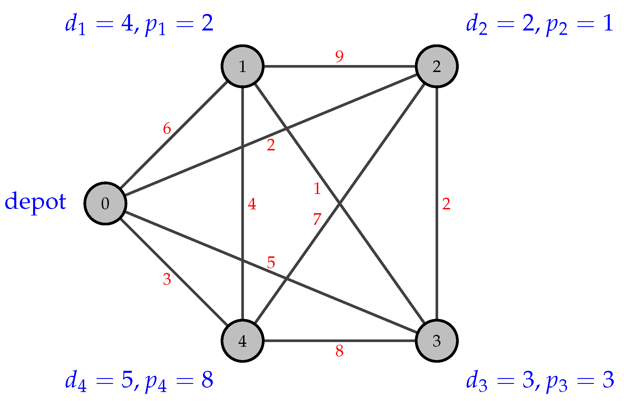
The algorithm continues to generate feasible solutions until a time limit is reached. The best set of routes found during this whole process is deemed to be the final solution. To illustrate the core of our algorithm, consider the running example presented in Figure 1 with 4 customers and the depot.

Assume that the random permutation is $unvisitedCustomers=3-4-1-2$ and that the capacity of the vehicle chosen to serve the route is $q=12$. Since $route$ is initially empty, the depot (i.e., node 0) is added to the route, and $trial$ is set to be the first customer from $unvisitedCustomers$ (i.e., customer 3). In this point, the route to be tested is $0-3-0$. We denote by $loa{d}_{ij}$ the cargo of the vehicle while traversing the arc $ij$. Note that the vehicle must leave the depot loaded with all deliveries of the customers on the route and, conversely, return to the depot with all pickup demands of these customers. In

Table 1. Vehicle load of the tentative route $0-3-0$.

	Depot	Customer 3
delivery	–	3
pickup	–	3
load	3	3

, we check the feasibility of the route:

• $loa{d}_{03}=d_3=3\le 12$;
• $loa{d}_{30}=loa{d}_{03}-d_3+p_3=3-3+3=3\le 12$.

Since the capacity constraint is satisfied throughout the route, customer 3 is effectively added to it and removed from $unvisitedCustomers=4-1-2$. At this point, we choose the next $trial$ customer either by the ordering of $unvisitedCustomers$ or by the nearest neighbor strategy, according to a probability $\rho$. Consider that the nearest neighbor strategy has been used to select the next customer this time, and thus customer 1 was chosen as $trial$. Therefore, the route to be tested is $0-3-1-0$, as presented in

Table 2. Vehicle load of the tentative route $0-3-1-0$.

	Depot	Customer 3	Customer 1
delivery	–	3	4
pickup	–	3	2
load	7	7	5

. We check its feasibility:

• $loa{d}_{03}=d_3+d_1=3+4=7\le 12$;
• $loa{d}_{31}=loa{d}_{03}-d_3+p_3=7-3+3=7\le 12$;
• $loa{d}_{10}=loa{d}_{31}-d_1+p_1=7-4+2=5\le 12$.

The capacity constraint remains satisfied all the way through the route, and therefore, customer 1 is added to it and removed from $unvisitedCustomers=4-2$. Again consider that $trial$ has been chosen by the nearest neighbor strategy, and thus customer 4 was selected as $trial$. Now the route to be tested is $0-3-1-4-0$, as shown in

Table 3. Vehicle load of the tentative route $0-3-1-4-0$.

	Depot	Customer 3	Customer 1	Customer 4
delivery	–	3	4	5
pickup	–	3	2	8
load	12	12	10	13

. We check its feasibility:

• $loa{d}_{03}=d_3+d_1+d_4=3+4+5=12\le 12$;
• $loa{d}_{31}=loa{d}_{03}-d_3+p_3=12-3+3=12\le 12$;
• $loa{d}_{14}=loa{d}_{31}-d_1+p_1=12-4+2=10\le 12$;
• $loa{d}_{40}=loa{d}_{14}-d_4+p_4=10-5+8=13\nleqq 12$.

However, in this attempt, the capacity constraint is violated. Customer 4 is not removed from $unvisitedCustomers=$ $\cancel{4}-2$ but is set to be infeasible (crossed out in the list). Assume now that $trial$ has been chosen by the ordering of $unvisitedCustomers$. In this case, the first customer not set as infeasible (customer 2) was selected as $trial$. Now the route to be tested is $0-3-1-2-0$, as presented in

Table 4. Vehicle load of the tentative route $0-3-1-2-0$.

	Depot	Customer 3	Customer 1	Customer 2
delivery	–	3	4	2
pickup	–	3	2	1
load	9	9	7	6

. We check its feasibility:

• $loa{d}_{03}=d_3+d_1+d_2=3+4+2=9\le 12$;
• $loa{d}_{31}=loa{d}_{03}-d_3+p_3=9-3+3=9\le 12$;
• $loa{d}_{12}=loa{d}_{31}-d_1+p_1=9-4+2=7\le 12$;
• $loa{d}_{20}=loa{d}_{12}-d_2+p_2=7-2+1=6\le 12$.

The capacity constraint is satisfied throughout the route, and therefore, customer 2 is added to it and removed from $unvisitedCustomers=\cancel{4}$. At this point, $unvisitedCustomers$ is not empty, and for that reason, we do not have a feasible solution yet. In addition, $unvisitedCustomers$ only contains customers that are set as infeasible, and thus the current route cannot be expanded. This route is then closed and incorporated to the current set of routes under construction. The feasibility of unvisited customers is reestablished ($unvisitedCustomers=4$), and a new route is opened. For the new route, assume that the capacity of the vehicle randomly chosen is $q=10$. The depot is added to the route, and $trial$ is set to be the first customer from $unvisitedCustomers$ (i.e., customer 4). The route to be tested is $0-4-0$, as shown in

Table 5. Vehicle load of the tentative route $0-4-0$.

	Depot	Customer 4
delivery	–	5
pickup	–	8
load	5	8

. We check its feasibility:

• $loa{d}_{04}=d_4=5\le 10$;
• $loa{d}_{40}=loa{d}_{04}-d_4+p_4=5-5+8=8\le 10$.

The capacity constraint is fulfilled, and therefore, customer 4 is added to the route and removed from $unvisitedCustomers=nil$. Since $unvisitedCustomers$ is empty, the route is closed and incorporated to the current set of routes. Finally, a feasible solution to the HVRPSPD is obtained.

Note that the computation time of the functions $nearestNeighbour$, $firstPossiblyFeasible$, and $checkRouteFeasibility$ is $O\left(n\right)$. Computing a feasible solution is $\mathsf{\Omega }\left(n^2\right)$ and $O\left(n^3\right)$ and, therefore, is quite efficient. The worst case scenario, however, is quite artificial, and the solution computation is indeed very fast.

3. Results

Our heuristic was implemented in Java 1.8.0. Experiments were performed on a PC Intel Core i7-7500 2.7 GHz 16 GB DDR3 RAM. Benchmark instances available in [13] were used in our computational study. These instances were grouped into 2 sets, each of them consisting of 14 instances. The first set contained problem instances with 10–100 customers, and the second set consisted of larger size problem instances with 150–550 customers.

3.1. Calibration of the Probability $\rho$

Since our heuristic is probabilistic, we randomly generated 4 new instances to calibrate the probability $\rho$ of choosing the nearest neighbor strategy. The instances were created in the same manner as described in [13]. For the first set, we generated 2 calibration instances with 50 and 100 customers and for the second set, another 2 calibration instances with 350 and 550 customers.

A range of values for the probability $\rho$ was set as $\{0.00,0.25,0.50,0.75,0.90,0.95,0.99,1.00\}$. Note that the bigger the $\rho$ value is, the more greedy the algorithm is with regard to the nearest neighbor strategy. Conversely, the smaller the $\rho$ value is, the more greedy the algorithm is with regard to the ordering of the customers. Nevertheless, the algorithm maintains its probabilistic fashion even for the extreme values of $\rho =0.00,1.00$ since permutations are generated at random. For each calibration instance and for each value of the probability $\rho$, we ran 10 executions of our algorithm using a time limit $\tau =60$ s. In Figure 2, we present best and average values obtained for the instance with 100 customers. The results show that our randomized algorithm performs significantly better as the probability $\rho$ increases. Very similar behavior was observed for the other 3 calibration instances.

3.2. Results for Benchmark Instances

In what follows, we present numerical results for the benchmark instances proposed in [13]. As suggested by the results of our calibration study, we used the 2 best values for the probability $\rho =0.99,1.00$ to perform our experiments. For each benchmark instance and for each value of the probability $\rho$, we ran 100 executions of our nearest-neighbor-based randomized algorithm (NNRA) with a time limit $\tau =60$ s. Detailed experimental results are provided as Supplementary Materials.

To compare our approach to other methods, we used IBM ILOG CPLEX 12.8 as the underlying solver of the formulation (1)–(12). A time limit of 3600 s of computation was set for the solver, and all other settings were preserved at their defaults. For each instance, the total number of vehicles found in the best solution of the NNRA, regardless of their types, was considered as the available quantity of each vehicle type in the formulation. In addition, we present the results obtained by the adaptive hybrid local search (HLS) of Avci and Topaloglu [13]. To the best of our knowledge, HLS presents the best results to date. It is important to point out that HLS uses a time limit of 7200 s (used together with a convergence criterion), whereas NNRA uses only 60 s. Note, however, that the authors performed their computational study on a PC Pentium 4 3.00 GHz, and according to the website https://cpu.userbenchmark.com, the Intel Core i7-7500 2.7 GHz is 244% faster considering the peak overclocked single core mixed speed.

In

Table 6. Comparative results for benchmark instances of Avci and Topaloglu [13]. HLS—adaptive hybrid local search; NNRA—nearest-neighbor-based randomized algorithm.

			CPLEX			HLS			NNRA ($\mathit{\rho }=0.99$)					NNRA ($\mathit{\rho }=1.00$)
inst.	$\mathit{n}$	$\mathit{t}$	sol.	bound	time (s)	best	avg.	time (s)	best	avg.	$\mathit{\sigma }$	$\Delta$(%)	time (s)	best	avg.	$\mathit{\sigma }$	$\Delta$(%)	time (s)
1-01	10	2	620.2	620.2	19.2	620.2	620.2	17.2	620.2	620.2	0.0	0.0%	0.3	665.0	665.0	0.0	7.2%	0.0
1-02	10	2	588.5	588.5	11.1	588.5	588.5	14.7	588.5	588.5	0.0	0.0%	0.1	589.2	589.2	0.0	0.1%	0.0
1-03	15	3	445.1	445.1	1969.7	445.1	445.1	22.7	445.1	445.1	0.0	0.0%	2.3	447.1	447.1	0.0	0.4%	0.0
1-04	15	4	460.4	408.4	3600.0	437.1	437.1	24.5	442.5	448.1	0.7	2.5%	25.5	453.9	453.9	0.0	3.8%	1.1
1-05	20	3	543.3	464.1	3600.0	494.0	498.9	27.1	500.8	502.7	1.2	0.8%	24.8	504.9	504.9	0.0	1.2%	0.3
1-06	20	4	640.8	512.9	3600.0	542.7	551.9	26.7	572.2	580.0	2.8	5.1%	24.5	583.1	583.1	0.0	5.7%	2.0
1-07	35	3	1814.4	987.6	3600.0	1108.2	1123.4	56.6	1155.9	1178.9	5.5	4.9%	29.0	1178.1	1180.6	4.1	5.1%	28.8
1-08	35	3	2263.9	1426.9	3600.0	1586.5	1601.2	54.7	1663.9	1681.2	6.8	5.0%	29.5	1663.9	1679.5	7.9	4.9%	29.4
1-09	50	3	2872.4	853.4	3600.0	964.4	990.2	91.4	980.3	993.4	4.9	0.3%	28.1	980.3	991.7	5.2	0.1%	31.2
1-10	50	2	–	1039.1	3600.0	1197.7	1228.6	95.8	1230.0	1267.6	8.9	3.2%	29.9	1240.2	1266.0	7.8	3.0%	29.3
1-11	75	3	–	1279.8	3600.0	1642.2	1673.9	143.8	1620.7	1667.0	14.4	−0.4%	28.2	1625.8	1659.2	14.2	−0.9%	27.9
1-12	75	2	–	800.6	3600.0	973.1	1002.5	164.9	1012.0	1045.1	10.7	4.2%	29.8	1010.9	1044.4	9.8	4.2%	28.1
1-13	100	2	–	1078.3	3600.0	1299.5	1353.5	288.5	1375.5	1417.0	10.6	4.7%	29.9	1372.2	1410.7	12.4	4.2%	30.2
1-14	100	2	–	1266.8	3600.0	1658.2	1678.2	310.3	1595.3	1635.3	10.8	−2.6%	32.1	1587.3	1628.5	12.7	−3.0%	30.8
2-01	150	3	–	1210.8	3600.0	1499.4	1624.5	592.5	1627.0	1654.4	17.2	1.8%	28.7	1627.0	1639.7	9.6	0.9%	30.4
2-02	150	3	–	1756.6	3600.0	2144.8	2152.5	548.9	2425.7	2479.1	20.3	15.2%	27.5	2369.7	2458.7	21.0	14.2%	31.9
2-03	200	3	–	–	–	3673.1	3688.8	831.6	3746.3	3830.9	31.8	3.9%	31.9	3669.8	3787.5	36.8	2.7%	31.7
2-04	200	2	–	1757.2	3600.0	2485.3	2682.5	919.4	2453.8	2528.8	22.0	−5.7%	32.9	2433.8	2506.0	21.0	−6.6%	31.3
2-05	250	3	–	–	–	2639.6	2810.0	1448.1	2683.8	2769.7	24.0	−1.4%	30.0	2682.6	2732.5	18.0	−2.8%	32.0
2-06	250	2	–	–	–	2549.8	2605.6	1521.3	2528.9	2634.8	28.6	1.1%	29.7	2516.4	2599.9	24.6	−0.2%	30.5
2-07	300	3	–	–	–	3205.0	3431.2	2440.4	2911.2	3000.9	29.0	−12.5%	31.4	2861.6	2959.4	26.1	−13.8%	31.1
2-08	300	2	–	–	–	3252.8	3364.6	2518.2	2867.7	2968.0	24.7	−11.8%	33.8	2861.8	2925.2	22.1	−13.1%	27.5
2-09	350	3	–	–	–	3457.9	3637.0	3770.1	3997.1	4136.4	41.5	13.7%	29.3	3937.2	4055.2	41.4	11.5%	29.8
2-10	350	2	–	–	–	3760.9	3897.5	3988.7	2622.7	2736.1	30.3	−29.8%	31.8	2613.8	2671.5	25.2	−31.5%	31.1
2-11	400	2	–	–	–	5809.5	6018.9	5662.4	3821.1	3941.9	37.9	−34.5%	30.5	3714.5	3855.6	36.1	−35.9%	30.2
2-12	400	2	–	–	–	4045.9	4447.0	5791.5	3441.5	3524.1	35.9	−20.8%	26.6	3397.1	3464.9	24.9	−22.1%	28.3
2-13	500	2	–	–	–	11,008.8	12,062.5	7200.0	8518.0	8794.8	87.3	−27.1%	30.5	8399.6	8660.7	89.7	−28.2%	30.9
2-14	550	2	–	–	–	12,762.0	13,046.3	7200.0	10,417.1	10,599.4	60.3	−18.8%	27.9	10,265.2	10,442.0	66.5	−20.0%	32.0

, along with the characterization of the instances (where n and t represent respectively the number of customers and the number of vehicle types), we present the results achieved by the alternative approaches. For CPLEX, we present the best feasible solution found (if any), the lower bound (if the solver was able to at least solve the root relaxation), and the solver computation time (if the solver was able to instantiate the model without an out-of-memory error). For HLS, we display the best and average solution values (over 10 executions) and the average computation time. For NNRA, we present the best and average solution values (over 100 executions), the standard deviation $\sigma$, and the percentage difference $\Delta$(%) between the results of the two heuristic algorithms, considering average solution values. A positive $\Delta$ value means that HLS obtained a better result, while a negative $\Delta$ value means that NNRA was able to find a better solution. We also present, for each instance, the average computation time to reach the best solution for each run (each execution, however, takes 60 s overall since we do not use any convergence criterion). The best known solutions are marked in bold font.

In Figure 3, we present the evolution of the computation time for each method as the size of the instances increases. Since the computational study for HLS was performed on a different machine, its computation time was rescaled by an appropriate factor of $2.{44}^{-1}$. And in Figure 4, we present a comparative study of the quality of the solutions obtained by each method.

4. Discussion

We begin the discussions of our experimental analysis stating that the exact approach is only able to cope well with the smaller instances. CPLEX finds the proven optimal solutions for the first 3 instances, but then its performance worsens dramatically. HLS and NNRA obtain the optimal solution for these 3 instances as well. None of the heuristic algorithms stands out from the other for all instances. Taking as reference the set of instances with 10–100 customers, HLS performs much better than NNRA, obtaining best solutions for 12 (out of 14) instances relatively quickly, while NNRA ($\rho =0.99$) obtains best solutions for 5 (out of 14). Note that, for the first 3 instances of set 1, the algorithms achieved the proven optimal solutions. NNRA ($\rho =1.00$), however, obtains best solutions only for 2 instances of set 1, suggesting that being too greedy with regard to the nearest neighbor strategy, in general, can lead to poor solutions. We would like to stress, however, that the solutions are not too bad if we consider the average percentage difference $\Delta$ between the solutions of HLS and NNRA for these instances (${\Delta }_{0.99}=1.98\%$ and ${\Delta }_{1.00}=2.59\%$ on average).

Concerning set 2 with larger size instances with 150–550 customers, NNRA outperforms HLS. In fact, NNRA ($\rho =0.99$) achieves best solutions for 9 (out of 14) instances, while NNRA ($\rho =1.00$) obtains best solutions for 10 (out of 14) instances. Moreover, the computation time used by HLS increases significantly, while NNRA uses the same time limit of 60 s without compromising the comparative quality of its solutions. In addition, the percentage difference $\Delta$ between the solutions for this set of larger instances is very expressive, now favoring NNRA (${\Delta }_{0.99}=-9.05\%$ and ${\Delta }_{1.00}=-10.33\%$ on average). The overall average percentage difference also favors our approach (${\Delta }_{0.99}=-3.53\%$ and ${\Delta }_{1.00}=-3.87\%$ on average).

As a final remark, although the comparative results have been expressive, we would like to point out that due to the simplicity of our algorithm and the relatively poor results it obtained for small instances, we believe that the optimality gap of the solutions may still be considerable for the larger-size instances. In fact, since our algorithm is very fast, it could be used to provide initial solutions to more sophisticated search methods. For instance, our solution could be used to boost the search method proposed by Avci and Topaloglu [13].

5. Conclusions

In this paper, we proposed a fast algorithm that constructs solutions to the HVRPSPD by probabilistic alternating between two greedy criteria to select the next customer to be visited: a given ordering of customers or the nearest neighbor strategy. Our results show that our approach performs better when the probability $\rho$ of using the nearest neighbor criteria is close to 1.

We used benchmark instances from the literature and compared our results to those obtained by a state-of-the-art algorithm. Our approach presented competitive results, particularly for the larger instances, improving several of the known solutions and running in a very short time.

As future work, we intend to adapt and apply our algorithm to tackle other classes of VRPs. In fact, the application to the VRPSPD (with a homogeneous fleet) is straightforward and, therefore, a natural research direction considering that the myriad of competitive approaches is broader. In addition, we envisage incorporating other criteria of exploring the solution space to find better solutions without compromising the simplicity of our algorithm. Another research direction is to use our algorithm to quickly obtain satisfactory feasible solutions and then apply local search methods to efficiently explore the neighborhood of these solutions.