Abstract
Visual object tracking is an important research topic in the field of computer vision. Tracking–learning–detection (TLD) decomposes the tracking problem into three modules—tracking, learning, and detection—which provides effective ideas for solving the tracking problem. In order to improve the tracking performance of the TLD tracker, three improvements are proposed in this paper. The built-in tracking module is replaced with a kernelized correlation filter (KCF) algorithm based on the histogram of oriented gradient (HOG) descriptor in the tracking module. Failure detection is added for the response of KCF to identify whether KCF loses the target. A more specific detection area of the detection module is obtained through the estimated location provided by the tracking module. With the above operations, the scanning area of object detection is reduced, and a full frame search is required in the detection module if objects fails to be tracked in the tracking module. Comparative experiments were conducted on the object tracking benchmark (OTB) and the results showed that the tracking speed and accuracy was improved. Further, the TLD tracker performed better in different challenging scenarios with the proposed method, such as motion blur, occlusion, and environmental changes. Moreover, the improved TLD achieved outstanding tracking performance compared with common tracking algorithms.
1. Introduction
Visual object tracking, as an important research field of computer vision, is a fundamental part of many computer vision systems, such as military navigation, human–computer interaction, unmanned aerial vehicle video analysis, dynamic behavioral recognition, intelligent medical treatment, and so on (see Figure 1) [1,2,3]. Given the location and extent of an arbitrary object, the task of visual object tracking is to determine the object’s location with the best possible accuracy in the following frames [4].
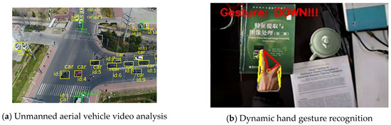
Figure 1.
Applications of visual object tracking.
Tracking results can be affected by several factors, such as illumination changes, occlusion, target nonrigid body deformation, and being out of view [5,6]. Choosing suitable features to represent the target is of great significance for visual object tracking to face the abovementioned challenging factors. Several authors have reported that color can adapt to plastic deformation well [7]. However, it is not easy for color to discriminate an object from the background [8]. Dalal and Triggs [9] studied the histogram of oriented gradient (HOG) descriptor to represent an object by capturing the edge or gradient structure and demonstrated its robustness in illumination changes. More complex features were also suggested to represent the visual object, such as scale-invariant feature transform (SIFT) and speeded up robust features (SURF) [10]. Additionally, particular features are used in tracking specific objects. For example, Haar-like descriptors are widely used in face tracking systems [11]. Because the appearance of an object may change during a video, model adaption is employed in most advanced trackers to make use of the information present in later frames.
Many researchers have shown great interest in visual object tracking and have proposed various trackers. For example, mean shift is a classical tracking algorithm. On the basis of the mean shift iterations, the most probable location of an object in a frame is found [7]. Particle-filtering-based trackers establish a certain model for objects and determine an object’s location by calculating the similarity between the particles and the target [12]. Correlation-filtering-based trackers show great advantages in tracking speed; these include the circulant structure kernel (CSK) tracker, the kernelized correlation filter (KCF) tracker, and the discriminative scale space tracker (DSST) [12]. As the performance of computers improve, deep learning has been applied to the field of computer vision. For example, Siamese and end-to-end networks have been widely used for tracking [13,14]. Among these trackers, the tracking–learning–detection (TLD) tracker proposed by Kalal et al. [15] introduced a novel tracking framework to solve the tracking problem. By combining a detector and a tracker with an online learning module, experiments showed that it performs well in long-term tracking. However, there are still some shortcomings that influence its actual application. The target is easily lost when the object is deformed or blurred. Further, the calculation is complicated, resulting in slow tracking speed.
To improve the performance of the TLD tracker, Lee et al. [16] studied the depth of images and applied it to enrich the object features. This proved to better represent an object in case of a complex background and is applicable to devices that can record depth information. A feature pool can be used for tracking a target to replace the object model in TLD and to select effective classifiers [17]. A feature pool helps to record the target characteristics more comprehensively. Nevertheless, collecting and maintaining the characteristics make the algorithm more complicated. Ye [18] reduced the image resolution to cut down the number of image patches to detect, thereby enhancing the tracking speed. However, reducing the resolution results in a loss of object features, especially when the object is small in the field of view. Although the improvements mentioned above optimize the TLD tracker, they fail to balance the robustness and real-time characteristics.
In this study, we optimized two aspects of the TLD: the tracking module and the detection module. A block diagram of the proposed algorithm is shown in Figure 2. The KCF tracker based on HOG was used to implement the tracking module. Failure detection was added for the response of KCF to identify if it fails to track the object correctly. As for the detection module, the detection strategy was adjusted based on the estimated object location provided by the tracking module. The detection module only needs to detect the scanning windows that are near the estimated location, so as to reduce the calculation and improve the tracking speed. If the tracking module loses the object, then the detection module detects the target in a full frame.
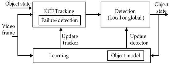
Figure 2.
Block diagram of the proposed algorithm. The kernelized correlation filter (KCF) tracker estimates the location of an object and posts it to the detector. The detection module detects the object just around the estimated location or scans the whole frame if the KCF fails to track. The learning module updates the object model and detector.
The rest of this paper is organized as follows: Section 2 briefly explains the principles of TLD; Section 3 introduces the implementation details of the algorithm proposed in this paper in detail; Section 4 describes the experiments and analyses, evaluating the improved TLD on benchmarks and comparing the performance with the original TLD as well as other trackers; and Section 5 concludes the paper.
2. TLD Tracking Framework
2.1. TLD Working Principle
TLD decomposes the tracking problem into three subtasks: tracking, learning, and detection. Each subtask is addressed by a single module and all the modules operate simultaneously. The block diagram of the TLD framework is shown in Figure 3.
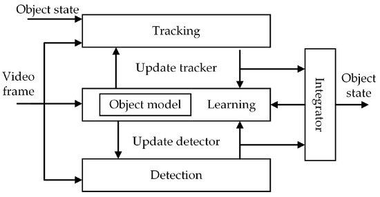
Figure 3.
Block diagram of the tracking–learning–detection (TLD) tracker. The tracking module follows the object from frame to frame. The detection module localizes the object in every frame. The object model is a collection of positive and negative patches. The learning module updates the object model and detection module. The integrator combines the results of the tracking and detection modules into one bounding box.
The tracking module is implemented by the median flow algorithm. As shown in Figure 4, the target is represented by a bounding box. Median flow firstly spreads points evenly within the bounding box and estimates the reliability of their displacements; then, half of the points with the most reliable displacements are selected as feature points. The motion of the object is obtained by the median of the displacements of the feature points [19]. The reliability of displacement is estimated by the normalized correlation coefficient (NCC) and the forward and backward error (FBE) using the pyramidal Lucas–Kanade algorithm. Figure 5 shows the definition of FBE. NCC compares the surrounding patch of the tracked point from the last frame (P1) to the current frame (P2), the definition of which is defined in Formula (1).
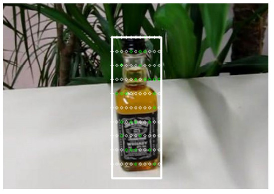
Figure 4.
Feature points of TLD. Corner points with light illumination change and small surrounding deformations are more likely to be selected as features points.
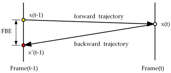
Figure 5.
The definition of forward and backward error (FBE). Point x(t − 1) is the location of an object in the last frame. Using the Lucas–Kanade tracker, x(t − 1) is tracked forward to the location x(t). Then, x(t) is tracked backward to the location x’(t − 1). The Euclidean distance between the initial point x(t − 1) and the end point x’(t − 1) is the FBE.
The learning module is developed by P-N learning [15]. It evaluates the error of the detector and updates the object model. According to the continuity of motion trajectory, P-experts analyze the negative patches and estimate false negatives using the tracking result, while N-experts estimate false positives by spatial structural correlation, which means the object will just appear in one place in a frame. The object model is a data structure that represents the object (positive) and its surroundings (negative). A patch will be added to the object model if its label estimated by the tracking module is different from that estimated by P-N experts [15]. The object module is used to update the classifiers in the detection module.
Detection is realized by cascading the variance classifier, ensemble classifier, and the nearest-neighbor classifier. The variance classifier rejects patches for which the gray-value variance is far smaller than that of the object model. The ensemble classifier generates pixel comparisons to detect the object. The nearest-neighbor classifier calculates the similarity of the performance between the patches and the object model. Finally, the patches that are most similar to the object model are sent to the integrator.
The integrator outputs the final bounding box of the TLD by combining the bounding boxes of the tracking and detection modules. The TLD framework guarantees reliable tracking through the tracking and detection modules. Further, the online object model is updated through the learning module. It can achieve long-term tracking with less prior knowledge and performs well if the object reappears after disappearing.
2.2. Disadvantages of TLD
In the tracking module of TLD, the feature points selected by the uniformly scattered points are not representative enough in describing an object’s features. If the object is rotated, obscured, or the background is complex, it may lose the tracking target [20].
The real-time performance of TLD is not good for its huge calculation requirement, which has difficultly meeting the actual application. The Lucas–Kanade tracker requires a large amount of calculation, especially when calculating the FBE, which needs twice that. In the detection module of TLD, a large number of scan windows are generated on the full frame. Even so, only a few of these patches have objects. For example, a 240 × 320 image will generate about 50,000 patches [15], which results in many calculations when passing through cascaded classifiers.
3. The Improved TLD Tracking Algorithm
To improve the real-time characteristics and robustness of TLD, the following measures are proposed in this paper: Firstly, the tracking module is implemented by the KCF tracker based on HOG descriptors. Then, failure detection with dynamic thresholds is introduced for the KCF tracker to check if it tracks the object correctly. The tracking module would neither return the estimated location of the object nor update its filter if a failure were detected. After that, the scanning frame is adjusted in the detection module. The detection module only detects the scanning windows around the predicted location of the object that is provided by the tracking module, considerably reducing the calculation requirements. If the tracking module fails to track the object, the detection needs to detect for the whole frame. An overview of the execution process of the proposed tracking algorithm is shown in Figure 6.
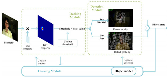
Figure 6.
The execution process of the proposed tracking algorithm.
3.1. HOG Descriptors
HOG is proposed to describe visual objects robustly, based on calculating well-normalized local histograms of image gradient orientations in a dense grid, as shown in Figure 7. To obtain the HOG of an object, the visual object is primarily divided into small connected regions called cell units. Then, the gradient or edge direction of each pixel is calculated in the unit. Finally, the collected histogram information is combined to obtain the HOG descriptors [9]. The following equations relate to the calculation of the pixel gradient:
where denotes the horizontal gradient, denotes the vertical gradient, is the gradient intensity, and represents the gradient direction.
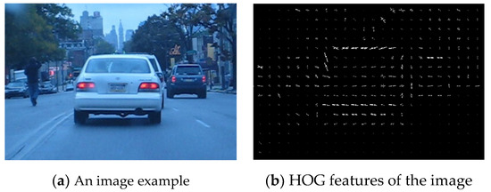
Figure 7.
Histogram of oriented gradient (HOG) features.
In each frame, HOG descriptors are obtained and applied to update the filter template of KCF. Compared with scattering points, HOG is easy to calculate and not sensitive to illumination changes or motion blur. In addition, HOG is obtained by fine orientation cells and their combination from larger regions. HOG descriptors can maintain robustness to a degree if slight plastic deformation or occlusion happens [9].
3.2. Implementing the Tracking Module with KCF
KCF solves the tracking problem by solving a simple grid regression problem [21]. It generates a large number of samples by cyclic shifts and trains the nonlinear prediction model of ridge regression to obtain a filter template. Then, the responses for the filter template are obtained on the current frame. Finally, the location of peak value for the response is regarded as the object’s position.
When implementing the tracking module by the KCF tracker, two adjustments are made. Firstly, KCF posts the estimated object’s location to the detection module instead of outputting a bounding box. A serious drawback of the KCF is its use of a fixed object bounding box, the size of which is the same as the extent in the first frame [8]. If the object’s scale changes or is occluded partially, KCF is unable to obtain the whole object or is easily influenced by excessive background. In the proposed tracking algorithm, KCF only estimates the object’s location and passes it to the detection module of TLD. The detection module generates all possible scales and shifts of the initial bounding box. For each window, the detection module decides the object state (presence or absence), then outputs a most reliable bounding box. The size of the bounding box is determined by the scanning window.
Secondly, the failure detection is appended before the KCF tracker outputs the location of the peak value in order to determine if the tracking module tracks the object correctly. The response of a location evaluates the similarity with the target. However, KCF cannot be aware of it and keeps tracking the bounding box in which the maximum response value is located. As a result, KCF may track the background, thus losing the target. In the failure detection, a dynamic threshold proposed by Liu [22] is set for the peak value of the response, and the equations are shown in Formula (6):
where the collection {Vi|i = 1, 2, …, n} represents the peak values recorded so far, u stands for the average of Vi, σ is the standard deviation of Vi, and θ is the threshold for the peak value of the current frame. KCF is considered to lose the target if the peak value is smaller than θ. λ is set empirically. In this study, λ was 4. It was observed that similar performance is achieved in the range (3–4).
If the peak value of the response is smaller than the threshold, the location of the peak value is marked as not reliable. Therefore, KCF would not update its filter template nor post the location of the peak value to the detection module. Figure 8 and Figure 9 illustrate the function of the failure detection. According to Figure 8, peak values were lower than thresholds from the 460th frame to around the 490th frame. As shown in Figure 9, KCF did track the wrong object when thresholds were larger than the peak value. If KCF is judged to track incorrectly, the tracking module will not pass the location of the peak value to the detection module.
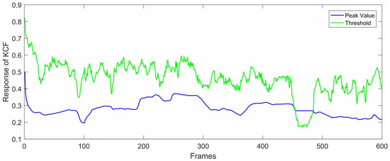
Figure 8.
The peak values and the threshold during a video sequence.
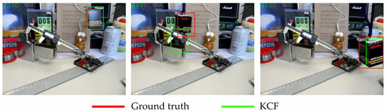
Figure 9.
The bounding boxes of KCF and ground truth. In the 491st frame, KCF tracked incorrectly and the peak value was lower than the threshold according to Figure 8 in the 250th and 550th frames.
3.3. Optimize the Detecting Strategy of the Detection Module
In the TLD framework, all possible scales and shifts of the initial bounding box are generated as a scanning-window grid. Deciding the presence or absence of the object for each window by cascading classifiers results in a great amount of calculations and slows down the tracking speed. In order to reduce the number of windows so as to improve the tracking speed, we proposed that the detection module just detects the windows around the estimated location by the tracking module, which is called “local detection” in this paper. If the tracking module fails to track the object, then the detection module detects the target in a full frame, called “global detection” in this paper. The difference between global detection and local detection is shown in Figure 10.
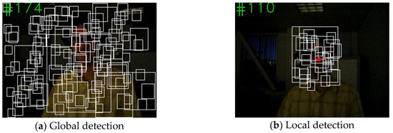
Figure 10.
The difference between global scan and local detection: (a) TLD generates detection windows on the full frame; (b) the improved TLD just generates windows around the predicted location (red point) calculated by the tracking module.
In this work, the range of local detection was centered on the estimated position of the object, and the size was 2.5 times the bounding box’s size on the last frame. That means the detection module only needs to detect windows, the coordinates of which are within this range. If the tracking module loses the target, the detection module needs to detect the target in a full frame. After global detection, if the detector finds the object, the tracking result is used to correct and initialize the KCF tracker. Otherwise, the improved TLD will not output the bounding box. To summarize, KCF is quick and local detection reduces many windows, thus improving tracking speed.
4. Experiments and Analysis
To evaluate the proposed algorithm, experiments were conducted on object tracking benchmark (OTB)50, which were manually annotated and widely used in previous works [23]. Firstly, the tracking accuracy of the improved algorithm was evaluated. On the one hand, the overlap rate (OR) was used to compare the tracking accuracy changes before and after the TLD algorithm was improved. On the other hand, the improved TLD was put to the full benchmark and evaluated by the precision curve and success rate curve. The performance of the improved algorithm was compared to other algorithms and their performance was examined in special scenarios. Finally, the tracking speed of TLD and the improved TLD was compared on the same computer and platform. Hereinafter, we refer to the improved TLD as “ours”.
4.1. Tracking Accuracy and Robustness
4.1.1. Comparison with the Original TLD
Considering that visual object was represented by a bounding box, the bounding box OR was chosen to measure the tracking accuracy between TLD and the improved TLD for the same video sequences. The more accurate the boundary of the object, the better it is for tracking. Formula (7) indicates the definition of OR:
where RT represents the estimated bounding box of the tracker, and RG stands for the ground truth bounding box. Likewise, average overlap rate (AOR) is the average of the overlap rate for a full video.
Experiments were conducted using several video sequences. Table 1 lists the results of four of the video sequences and includes the frames, AOR, and the growth rate of AOR. According to Table 1, the proposed algorithm showed better tracking accuracies. Figure 11 shows the results of the overlap rate in every frame in detail; the vertical axis shows the overlap rate and the horizontal axis represents the frame number. An OR of 0 means that the tracker lost the target. As can be seen from Figure 11, the overlap rate fluctuated during a video. The overlap rates of the proposed algorithm exceeded TLD in the majority of frames. Furthermore, the number of times the target was missed was reduced after the improvements were implemented.

Table 1.
Average overlap rate (AOR) of video sequences.
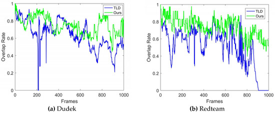
Figure 11.
Bounding box overlap rate per frame in two sequences.
Figure 12 indicates that both spatial shifts and scales will result in a low overlap rate. The tracker cannot obtain the accurate state of an object if only part of the object is included in the bounding box. Similarly, too much background may make the tracker mistake then background as a part of the object. Since the patch may be added into the object model in TLD, the tracking precision in the following frames will be influenced by the previous results. Especially for the tracking module of the original TLD, the target feature points are obtained by spreading the points uniformly and calculating the FBE, which is not representative and robust enough to describe the object itself. In contrast, the proposed algorithm uses HOG descriptors in the tracking module, which pays more attention to the statistical characteristics and is insensitive to interference from individual points. A reliable tracking module will lay a good foundation for other parts of a tracker. Thus, the improved TLD achieved better tracking accuracy. Nevertheless, HOG descriptors have drawbacks. They rely on the spatial configuration of the target and perform poorly if the object is severely plastic-deformed. A combination of multiple features is a possible way to solve the problem and worth further research in the future.
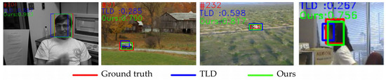
Figure 12.
Frames with very different overlap rates.
4.1.2. Experiments on OTB50
Quantitative analysis for the proposed algorithm was obtained based on the full benchmark OTB50. The precision curve and success rate curve were chosen to evaluate the performance of the trackers. The left part of Figure 13 shows the precision curves, and the x-axis is the center location error (CLE), the Euclidean distance between the center of the target box and the ground truth. A frame can be considered correctly tracked if the CLE is within a distance threshold. The precision curve shows the percentage of correctly tracked frames for a range of distance thresholds. In the legend of the precision curves, the value in the square brackets is the precision value at a location threshold of 20 pixels. Similarly, the success rate curve presents the percentage of correctly tracked frames for a range of overlap rates. In the legend of success plots, the value in the square brackets is the success rate value in the threshold of 0.5.
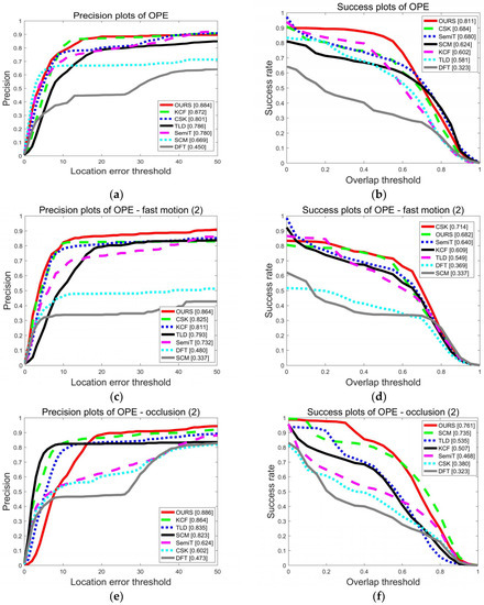
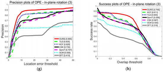
Figure 13.
Precision and success plots on the object tracking benchmark (OTB): (a) precision plots of the one-pass evaluation (OPE), (b) success plots of OPE, (c) precision plots of fast motion, (d) success plots of fast motion, (e) precision plots of occlusion, (f) success plots of occlusion, (g) precision plots of in-plane rotation, and (h) success plots of in-plane rotation.
Figure 13 shows the tracking performance on the full dataset. The improved TLD was compared with the original TLD as well as other advanced tracking algorithms, including CSK, semi-supervised tracker (SemiT), tracking via sparsity-based collaborative model (SCM), and distribution fields for tracking (DFT) [23]. In addition to the average performance of the algorithm, performances in challenging scenes were also compared, including fast blur, occlusion, and in-plane rotation. It can be seen from Figure 13a,b that the improved TLD performed better than before. In Figure 13a, when the threshold was 20 pixels, the precision increased by 12.47%. In Figure 13b, when the threshold was 0.5, the success rate increased by 39.59%. In motion-blurred scenes, the tracking accuracy was greatly improved when the accuracy requirements were strict. For example, as shown in Figure 13c, when the threshold was 10, the accuracy of the TLD was 45%. Nevertheless, the improved TLD reached 80%. In the case of occlusion and in-plane rotation, our algorithm performed best, even exceeding KCF. This can be attributed to two reasons. For one thing, the addition of failure detection can help to avoid tracking the background. Also, it is the detection module of the TLD framework that detects and corrects the KCF tracker.
Compared with other common algorithms on OTB, the performance of the improved TLD was excellent. In order to more intuitively observe the performance of different trackers in challenging scenes, five representative videos were selected for experiments. The basic information of these five groups of video sequences is shown in Table 2.
Table 2.
The properties of the five videos.
Qualitative comparisons were carried out to compare tracking performances in challenging scenes from these sequences. As can be seen from Figure 14a that when the object was blocked, TLD contained too much background in its bounding box, resulting in losing track of the target in the following frames. Due to the object model, TLD tracked the object again after occlusion disappeared. However, CSK and DFT failed to track the real target. Ours performed best in this sequence, tracking accurately even when occlusion was severe.
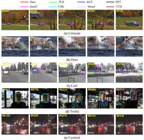
Figure 14.
A qualitative comparison of our approach with seven common trackers.
In Figure 14a,c, the common challenge depicted is scale change. Our algorithm had the best adaptability. In Figure 14a, when the object became larger, VDT, SemiT, KCF, and Struck kept tracking a part of the object. In Figure 14c, ours tracked for longest time with high accuracy; KCF was the second best. Because of the fixed box size, KCF could not adapt to the scale changes. Too much unrelated background was included in the bounding box when the object became smaller. Inappropriate sizes of the bounding box led to low tracking accuracy and even a lost target, as in the 792nd frame in Figure 14c. Ours performed well because it only passed the predicted location of the object from the tracking module to the detection module. The size of the bounding box was determined by the detection module and the scanning-window grid. Further, the failure detection helped to avoid tracking the background. If the detection module also does not find the object, the tracker will not output a bounding box and KCF will not update the filter template.
TLD mistook the similarity as the object in Figure 14c, while ours did not. It could be inferred that the tracking module of TLD lost the target, so the detection module tracked the similarity by mistake. However, our tracking module was more robust and tracked correctly; then, the detection module detected around the predicted location. Therefore, ours tracked successfully.
The difficulty in Figure 14b is motion blur. Ours, CSK, and Struck tracked the object but others lost it. The common difficulties of Figure 14d,e are illumination changes and background clutter. Most trackers kept tracking the object but with different offsets. Both motion blur and illumination change will make the texture of an object surface change, while occlusion may block the feature points [18]. For TLD, the complex background weakened the function of the first-level variance classifier, which resulted in many calculations for the next two classifiers. Further, the change of the surface affected the extraction of feature points. Finally, TLD tracked at a low speed and with poor accuracy. DFT uses raw intensity and locates an object by local optimum search, which makes it easy to lose the object when there is background clutter [24]. Our, KCF, and Struck trackers use gradient features, thus tracking with strong robustness to brightness changes and motion blur.
4.2. Tracking Speed
Real-time characteristics were evaluated by frames per second (FPS), the unit of which is frames/s. The tracking speeds of the same algorithm vary across different computer configurations. So, these experiments were all done on the same computer. Moreover, the FPS values were the average of repeated tests. Table 3 shows the number of successfully tracked frames and FPS.
Table 3.
The number of successfully tracked frames and frames per second (FPS).
As shown in Table 3, compared with the original TLD, the improved TLD not only increased the number of successfully tracked frames but also enhanced the FPS. Tracking speed is directly related to the tracking algorithm. It is also affected by the image size, object scale, and color. Large images will generate more scan windows and every patch is larger, resulting in longer tracking time. It can be seen that the FPS of “Girl” was quicker than that of the others. Analyzing the FPS of the improved TLD, the increase in FPS was different among video sequences. If the target was relatively small in the image, the advantage of local search was more obvious. More specifically, the effect on reducing the amount of calculations was more significant. Examples include “CarScale” and “Redteam”.
Moreover, it was observed that the tracking speed slowed down with the accumulation of patches in the object model. Further, early samples were less representative. Therefore, sample management is a meaningful issue in further research. More challenging applications are available on the basis of a real-time tracker. For example, multitarget tracking is a direction worth trying.
5. Conclusions
TLD provides an effective framework for solving long-term tracking problems. However, its practical applications are limited due to the complicated calculations and poor real-time performance. To improve the robustness and tracking speed of TLD, several steps were made in this study. Firstly, the tracking module was implemented by the KCF tracker based on HOG descriptors. Secondly, failure detection was added to check if KCF tracks the object correctly. Finally, the detection strategy was optimized. Local detection was carried out to reduce the detecting windows, so as to improve the tracking speed. Full-frame detection is not necessary until the KCF fails to track an object. Comparative experiments were carried out on the benchmark to evaluate the improved algorithm. Comparing the results of TLD with other advanced tracking algorithms showed that the proposed method provides improvements in terms of accuracy, robustness, and real-time performance. Further, it achieves outstanding tracking performance compared with the common tracking algorithms.
Author Contributions
Conceptualization, X.Z. and S.F.; methodology, X.Z. and S.F.; software, X.Z.; validation, X.Z., Y.W., and W.D.; investigation, Y.W. and W.D.; data curation, X.Z., Y.W., and W.D.; writing—original draft preparation, X.Z.; writing—review and editing, X.Z., S.F., Y.W., and W.D.; supervision, S.F. All authors have read and agreed to the published version of the manuscript.
Funding
This research received no external funding.
Conflicts of Interest
The authors declare no conflict of interest.
Abbreviations
The following abbreviations are used in this manuscript:
| TLD | Tracking–learning–detection |
| KCF | Kernelized correlation filters |
| HOG | Histogram of oriented gradient |
| SITF | Scale-invariant feature transform |
| SURF | Speeded up robust features |
| CSK | Circulant structure kernel |
| DSST | Discriminative scale space tracker |
| FBE | Forward and backward error |
| NCC | Normalized correlation coefficient |
| OTB | Object tracking benchmark |
| OR | Overlap rate |
| AOR | Average overlap rate |
| CLE | Center location error |
| FPS | Frames per second |
| SemiT | Semi-supervised tracker |
| SCM | Tracking via sparsity-based collaborative model |
| DFT | Distribution fields for tracking |
References
- Cao, S.; Wang, X. Real-time dynamic gesture recognition and hand servo tracking using PTZ camera. Multimed. Tools Appl. 2019, 10, 78. [Google Scholar] [CrossRef]
- Yu, H.; Li, G.; Zhang, W.; Huang, Q.; Du, D.; Tian, Q.; Sebe, N. The Unmanned Aerial Vehicle Benchmark: Object Detection, Tracking and Baseline. Int. J. Comput. Vis. 2019. [Google Scholar] [CrossRef]
- Zhang, W.; Luo, Y.; Chen, Z.; Du, Y.; Zhu, D.; Liu, P. A Robust Visual Tracking Algorithm Based on Spatial-Temporal Context Hierarchical Response Fusion. Algorithms 2019, 12, 8. [Google Scholar] [CrossRef]
- Wang, Q.; Zhang, L.; Bertinetto, L.; Hu, W.; Torr, P.H. Fast online object tracking and segmentation: A unifying approach. In Proceedings of the IEEE Conference on Computer Vision and Pattern Recognition (CVPR), Los Angeles, CA, USA, 15–21 June 2019; pp. 1328–1338. [Google Scholar]
- Yang, S.; Xie, Y.; Li, P.; Wen, H.; Luo, H.; He, Z. Visual Object Tracking Robust to Illumination Variation Based on Hyperline Clustering. Information 2019, 10, 26. [Google Scholar] [CrossRef]
- Hu, Z.; Shi, X. Deep Directional Network for Object Tracking. Algorithms 2018, 11, 178. [Google Scholar] [CrossRef]
- Medouakh, S.; Boumehraz, M.; Terki, N. Improved object tracking via joint color-LPQ texture histogram based mean shift algorithm. Signal Image Video Process. 2018, 12, 3. [Google Scholar] [CrossRef]
- Bertinetto, L.; Valmadre, J.; Golodetz, S.; Miksik, O.; Torr, P.H.S. Staple: Complementary Learners for Real-Time Tracking. In Proceedings of the International Conference on Computer Vision and Pattern Recognition (CVPR), Las Vegas, NV, USA, 27–30 June 2016; pp. 1401–1409. [Google Scholar]
- Dalal, N.; Triggs, B. Histograms of oriented gradients for human detection. In Proceedings of the International Conference on Computer Vision and Pattern Recognition (CVPR), San Diego, CA, USA, 20–25 June 2005; pp. 886–893. [Google Scholar]
- Yu, L.; Ong, S.K.; Nee, A.Y. A tracking solution for mobile augmented reality based on sensor-aided marker-less tracking and panoramic mapping. Multimed. Tools Appl. 2016, 75, 6. [Google Scholar] [CrossRef]
- Visakha, K.; Prakash, S.S. Detection and Tracking of Human Beings in a Video Using Haar Classifier. In Proceedings of the International Conference on Inventive Research in Computing Applications (ICIRCA), Coimbatore, India, 11–12 July 2018; pp. 1–4. [Google Scholar]
- Nishimura, H.; Nagai, Y.; Tasaka, K.; Yanagihara, H. Object Tracking by Branched Correlation Filters and Particle Filter. In Proceedings of the 2017 4th IAPR Asian Conference on Pattern Recognition (ACPR), Nanjing, China, 26–29 November 2017; pp. 79–84. [Google Scholar]
- Dai, K.; Wang, Y.; Yan, X. Long-term object tracking based on siamese network. In Proceedings of the 2017 IEEE International Conference on Image Processing (ICIP), Beijing, China, 17–20 September 2017; pp. 3640–3644. [Google Scholar]
- Valmadre, J.; Bertinetto, L.; Henriques, J.; Vedaldi, A.; Torr, P.H. End-to-end representation learning for correlation filter based tracking. In Proceedings of the IEEE Conference on Computer Vision and Pattern Recognition (CVPR), Honolulu, HI, USA, 21–26 July 2017; pp. 2805–2813. [Google Scholar]
- Kalal, Z.; Mikolajczyk, K.; Matas, J. Tracking-learning-detection. IEEE Trans. Pattern Anal. Mach. Intell. 2012, 34, 1409–1422. [Google Scholar] [CrossRef] [PubMed]
- Lee, J.H.; Jung, H.J.; Yoo, J. A real-time face tracking algorithm using improved camshift with depth information. J. Electr. Eng. Technol. 2017, 2, 5. [Google Scholar]
- Prasad, M.; Zheng, D.R.; Mery, D.; Puthal, D.; Sundaram, S.; Lin, C.T. A fast and self-adaptive on-line learning detection system. Procedia Comput. Sci. 2018, 144, 13–22. [Google Scholar] [CrossRef]
- Ye, Z.D. Improvement and Implementation of Self-learning Visual Tracking Algorithm for Android. Master’s Thesis, Southeast University, Nanjing, China, 2017. [Google Scholar]
- Kalal, Z.; Mikolajczyk, K.; Matas, J. Forward-backward error: Automatic detection of tracking failures. In Proceedings of the 2010 20th International Conference on Pattern Recognition, Istanbul, Turkey, 23–26 August 2010; pp. 2756–2759. [Google Scholar]
- Taetz, B.; Bleser, G.; Golyanik, V.; Stricke, D. Occlusion-aware video registration for highly non-rigid objects. In Proceedings of the IEEE Winter Conference on Applications of Computer Vision (WACV), Lake Placid, NY, USA, 7–10 March 2016; pp. 1–9. [Google Scholar]
- Henriques, J.F.; Caseiro, R.; Martins, P.; Batista, J. High-speed tracking with kernelized correlation filters. IEEE Trans. Pattern Anal. Mach. Intell. 2014, 37, 583–596. [Google Scholar] [CrossRef] [PubMed]
- Liu, Y.F.; He, Y.H.; Zhang, W.; Cui, Z.G. Research on KCF target loss early warning method based on outlier detection. CEA 2018, 54, 216–222. [Google Scholar]
- Wu, Y.; Lim, J.; Yang, M.H. Online Object Tracking: A Benchmark. In Proceedings of the IEEE Conference on Computer Vision and Pattern Recognition (CVPR), Portland, OR, USA, 23–28 June 2013; pp. 2411–2418. [Google Scholar]
- Fang, Y.; Yuan, Y.; Li, L.; Wu, J.; Lin, W.; Li, Z. Performance evaluation of visual tracking algorithms on video sequences with quality degradation. IEEE Access 2017, 5, 2430–2441. [Google Scholar] [CrossRef]


© 2020 by the authors. Licensee MDPI, Basel, Switzerland. This article is an open access article distributed under the terms and conditions of the Creative Commons Attribution (CC BY) license (http://creativecommons.org/licenses/by/4.0/).