1. Introduction
Nowadays, information sciences are used in almost all areas of our daily life. As a result, information technologies are, more than ever, a strategic resource for entities and activities such as strategic decision making, learning, modeling, design, development of decision algorithms, integration and validation of strategies.These activities are at the cutting edge of technology and research and involve several fields and skills. The decision-making process is crucial in all of these activities. Decision-making is of primary factor in several organizations such as companies, families, governments, armies, etc. Its importance and its relevance vary from one sector to another. Companies that face an economic, social and competitive environment must have management systems that will allow them to make correct decisions as they engage their future. In the military field, and for several centuries, conflicts between nations have given rise to several wars which have multiple origins.
When the participants of a war have similar properties in terms of quantities-of-interest, values, resources, technologies, the war is said to be symmetrical from a strategic decision-making perspective. However, symmetrical wars are hardly observed in practice. In general, asymmetric wars are observed. These include wars between two nations, a strong nation against a weak enemy with very few resources or against materially insignificant combatants, who use the weaknesses of this nation to achieve their specific goals.
In this context, nations are faced with large-scale decision-making when preventing, negotiating, combating different groups, because they can act and harm nations at anytime. Nations have some resources and often a certain level of information about the enemy. However, how can one use this information efficiently without danger or significant loss of resources in order to win the battles or to remedy these battles constantly, or to be a threat to the enemy away? So, for the armed forces of a nation, decision-making becomes one of the most important things, because a bad decision would bring huge consequences and heavy losses. They are faced with several scenarios, each of which has an implementation and simulation time, allowing them to use the data from this simulation and to make decisions. However, decision-makers must make decisions within a specific time frame. In terms of decision-making, there is no such thing as coincidence. It is important to make decisions with a preliminary study, to know what will happen, taking into account the assumptions. Models are used to predict a situation over time and to evaluate the result in order to make well-considered decisions. So, research around strategic decision-making is a real challenge and allows us to better prepare for the future by developing innovative concepts. Strategies for decision-making have been widely explored, but as science evolves day by day, research is devoted to improving existing strategies.
In this context, we are interested in studying new distributed learning methods for better resource allocation strategies and working on the development and implementation of optimal strategy learning algorithms. To do that, we propose the following steps:
Review of the existing learning algorithms with complexities and performance analysis;
Selection of state-of-the-art solutions and their implementation;
Design and development a new optimal solution using advanced learning methods;
Carry out validation scenarios;
Validation of the proposed solution on the basis of objective criteria.
In the remainder of this paper, we will first review the literature to present a background on game theory and strategies algorithms. Then, we will present the formulation of a new problem and elaborated algorithm to solve it. Subsequently, we will present a case study to evaluate algorithms highlighted in the paper. Finally, we conclude with the discussion outlining interpretations, contribution and limitations of our study directions for further research.
2. Background
Resource allocation and decision-making have been the subject of several studies. We review different resource allocation strategies and highlight advantages and shortcomings.
2.1. Game Theory
Game theory studies interactive decision-making problems. Basically, a game in strategic form is given by the description of the interest of the players and the constraints which weigh on the strategies that players can choose [
1]. A game essentially includes the following four elements [
2]:
A set of players: this set specifies which decision-makers or players are involved in the game. A player can be a single individual or a group of individuals making a decision. Each player optimizes his/her quantity-of-interest, that is to say that each player is aware of the alternatives, anticipates the unknown elements, has clear preferences and deliberately chooses his/her action after an optimization process.
A set of rules: it is the course of the game, the procedure to follow and the possibilities of action or strategies (set of moves or choices of the players) offered to the players.
A set of issues: each outcome is the consequence of the actions taken by the players.
A set of gains: the outcomes determine the winnings distributed to players, the value (winnings or utility function) for each player of the different possible outcomes of the game. The notion of utility or utility function is modeling the interest that a player finds in an outcome. It is generally represented with a real number or real numbers so that a comparison can be made.
Game theory is a set of tools allowing one to analyze interactions in which players (physical person, company, animal, state, machine, a group etc.) make decisions depending on the anticipations that it forms on what one or more other players will do. We refer the reader to [
3,
4,
5,
6,
7,
8,
9,
10,
11] for more details and recent applications of game theory in deep learning. One of the objectives of game theory is to design and model situations requiring decision-making, to determine an optimal strategy for each of the players, to predict the outcomes of the game and to find out how to achieve an optimal situation. Game theory analyzes and predicts future actions using scientific means to create models of behavioral analysis and neglected at the base of external events, in particular natural ones, which have as much influence as other players in the game [
12]. However, with the rapid evolution of this discipline, several of these forms of external events have already been taken into account in game theory over the past thirty years. The most common types of games can be found in [
2]:
Cooperative and non-cooperative games: a cooperative game is a situation where communication and agreements between players are allowed before the game. Thus, all the agreements between the players are respected and also all the messages formulated by one of the players are transmitted without modification to the others. On the other hand, the assessment of the situations by a player is not disturbed by the preliminary negotiations. Otherwise, we consider that the game is non-cooperative.
Simultaneous and sequential games: a simultaneous or strategic game is a situation where each player chooses his/her complete action plan once and for all at the start of the game. Consequently, the choices of all the players are simultaneous. So, when making a choice, the player is no longer informed of the choices of other players.
On the other hand, a sequential game specifies the exact course of the game; each player considers his/her action plan, not only at the start of the game, but also whenever (s)he must actually make a decision during the course of the game. In general, the simultaneous games are represented in the form of a table and the sequential games are represented by a game tree which allows the complete representation of the structure and the progress of the game.
Finite games: a game is finite if the set of strategies for each player is finite. That is to say, the sets of strategies are finite sets.
Zero-sum games and non-zero-sum games: zero-sum games are two-player games in which the sum of the gains and losses of the two players is zero. They are also called strictly competitive games because the interest of one player is strictly opposed to the interest of the other; therefore, the conflict is total and there is no possible cooperation (what wins one is lost by the other). Similarly, a non-zero sum game is a game in which the sum of the winnings is different from zero (0). It is either positive or negative.
Repeated games: the repeated games are simultaneous games which are played several times in a row. The game conditions do not change (the number of players and their strategies and also the utility functions of the strategies).
Games with full information and games with incomplete information: the information available to players every time they have to choose an action is a very important dimension of games. It has a decisive influence on the evaluation of strategies by players and even on their perception of strategies. A game is full information if all players know the structure of the game perfectly. It is incomplete information if at least one of the players does not know its structure perfectly.
Perfect memory games and imperfect memory games: the game is perfect memory if each player is perfectly informed of the past actions of other players. When a player ignores some of the choices that were made before his choice, the game is an imperfect memory game.
The same game can belong to several types at the same time and according to different contexts of interactions we can classify the games into three big families based on: the type of cooperation between the players (cooperative or non-cooperative), development over time (simultaneous or sequential), information available to players (perfect or imperfect information and complete or incomplete) [
1]. There are two basic forms to represent a game [
1]:
Normal Form: a game in normal form is described by the following elements:
- –
A set of n players:
- –
For each player i, , a set of strategies Si, which contains all the possible strategies for this player. if is a particular strategy for player i. Therefore, if strategies are available for player i. If each player i chooses a strategy , we can represent the result (or strategy profile) of the game by a vector which contains all these strategies:
- –
For each player i, a gain function, , which represents the preferences of player i by giving the value for player i of each result of the game: . It’s a real number:
This form is suitable for the representation of simultaneous games which can be represented in the form of a table.
Extensive form: a game in extensive form is given by a game tree containing an initial node, decision nodes, terminal nodes and branches connecting each node to those which succeed it.
- –
A set of players, indexed by .
- –
For each decision node, the name of the player who has the right to choose a strategy at this node.
- –
For each player i, the specification of all the actions allowed at each node where (s)he is likely to make a decision.
- –
The specification of the winnings of each player at each terminal node.
Sequential games where decisions are made at different times and each player can be made to play multiple times are shown in extensive form.
There are several resolution methods:
Elimination of equivalent strategies: Redundant strategies are called equivalent strategies, and after their elimination, we get the reduced normal form of the game.
Elimination of dominant strategies: Some of the players’ strategies may be worse overall than others. One would expect that these strategies would never be chosen by rational players. We can then choose to eliminate them immediately from the game.
Nash equilibrium: Equilibrium is a situation where everyone’s expectations are realized: the opponent does what I have planned, and I act in order to make the most of it. The most commonly used equilibrium in game theory is the Nash equilibrium. This is a situation where no player has any interest in unilaterally deviating from their strategy when other players continue to play the same strategies.
It has several resolution methods and has some shortcomings (non-existence of a pure Nash equilibrium and the existence of several Nash equilibria).
There are other resolution methods, such as: perfect equilibrium in subsets, minimax solution, correlated equilibrium, etc.
2.2. Game Theory and Decision Making
The decision is an act by which a decision-maker makes a choice between several options, allowing one to bring a satisfactory solution to a given problem or the execution of an action or a project with all the consequences that this decision could generate. A decision is a resolution you make about something. Each decision is the result of a complex process which, as a rule, involves two ways of thinking: looking back to understand the past (it is the study of what exists) and looking further to predict the future. The nature of the decisions to be made affects how the decision-making process will unfold. Some subjects have little stake, that is to say that the consequences are low. Some, on the contrary, have a strong stake. Any decision-making must include a great knowledge of the problem. By analyzing and understanding it, it is then possible to find a solution. Of course, when faced with simple questions, decision-making takes place practically on its own, and without any complex or profound reasoning. On the other hand, in the face of decisions that are more transcendent for life, the process must be thought through and treated [
13]. Therefore, we generally use game theory, either to analyze market structures, or to study the behavior of different actors (states, institutions, companies, etc.) through a formalization of their understanding process, of coopetition, partial atruism, spitefulness, coalition, rivalry or conflict.
2.3. Different Games of Colonel Blotto
Colonel Blotto’s “Blotto Game” is a conflict between two (02) military forces. This is a situation that has been modeled in game by game theory, in order to solve the problem of optimal allocation of resources. The situation is such that two military forces are in conflict. Each has its resources which it must allocate during the confrontation, which can take place on one or more fronts.
Both players have resources to allocate on a number of battlefields. The rules of the game are defined and depend on the type of game and its configuration.
The strength allocated to each battlefield must be positive. For player
i, all of the possible force assignments across the
n battlefields are designated by [
14]:
So, using game theory, the conflict situation is modeled into a game called “Colonel Blotto’s game” with the following elements:
The military forces are represented by players,
The decisions they make are represented by actions or (pure) strategies,
The rules of the game define the course of the game, at the end of which, the winner and the loser will be known.
2.3.1. Symmetrical Games
The zero-sum game: Colonel Blotto’s zero-sum game comes from [
15]. It is a constant sum game involving two players,
A and
B, and
n independent battlegrounds. Player
A has
units of force to be dispatched between the battlefields, and Player
B has
units. Each player must distribute his/her forces without knowing the distribution of the opponent. If
A sends
units and
B sends
units to battlefield
k, the player with the higher strength level wins on battlefield
k. An equilibrium of this game is a pair of
n-varied distributions (a varied distribution with
n dimensions) and the first solutions appear in [
15] in 1938, which solve the problem in the case of
and
(the number of battlefields is 3 and the number of resources of both players is equal).
In the model of this game, two players A and B simultaneously assign their forces and respectively on a finite number of homogeneous battlefields. Each battlefield has a gain of . Each player’s gain is the sum of the winnings across all battlefields or, equivalently, the proportion of battlefields to which the player sends a higher level of strength. In the case where both players allocate the same level of force to a battlefield, it is assumed that player B ((s)he is assumed to be the opponent of the one who establishes the game, so for him/her it is victory or defeat but no draw because the latter is considered a defeat) wins this battlefield and all resources are to be used.
The non-zero sum game: After the constant sum game, Roberson and Kvasov presented a non constant sum version of the classic Colonel Blotto game [
16]. In Borel’s original formulation of the Colonel Blotto game, player resources are “use them or lose them”, in the sense that all resources that are not assigned to one of the contests are lost. The Kvasov non-constant version of the Colonel Blotto game makes it more flexible to use or lose this feature.
As a model, two players, A and B, simultaneously enter offers in a finite number , of independent battlefields. Each field has a common value for each player. Each player has a fixed level of available resources which may or may not be equal, but here, we will focus on the case where they are unequal. In the case where the players allocate the same level of force in a given field, it is assumed that player B wins on this field, otherwise the player who has used a greater number of resources wins this battlefield.
As long as the players’ budgets are not too asymmetrical, there is a equilibrium in the game. However, if the players’ budgets are sufficiently asymmetrical, new joint distributions of equilibria must be built entirely.
The game with heterogeneous battlefields: Colonel Blotto’s game with heterogeneity in battlefield values is a variant of the games of Colonel Blotto previously seen, which presents a new geometric method for constructing equilibrium distributions with heterogeneous battlefields [
17]. We have the two-player model
A and
B with identical budgets
. The players have to allocate their resources on
battlefields indexed by
. For both players, the value of the battlefield
i is
and each player has his/her own value which (s)he assigns according to the importance of this field from his/her point of view (the fields do not have the same values for the two players).
Each player seeks to maximize the overall value of the battlefields captured, by trying to win the most fields and prefers those with high values. The rules are like for the other games of colonel Blotto—the one who allocates a high number of forces (resources) wins this field, and when a tie occurs, it is assumed that player B wins this field.
2.3.2. Asymmetrical Games
Colonel Blotto’s asymmetrical game model is such that the game is a constant sum involving two players, A and B, and n independent battlefields. A distributes units of force among the battlefields in a non-decreasing manner and B distributes units of force among the battlefields in a non-decreasing manner. Each player distributes forces without knowing the distribution of the opponent. The player who provides the highest level of force (resources) to a battlefield wins that battlefield. If both players deploy the same force on a battlefield, we declare that the battle on that field must be a draw, and the reward for that battlefield is equally divided between the two players. The gain for each player is the proportion of battlefields won.
Colonel Blotto’s asymmetrical game was a step forward, but has its shortcomings. Beyond three battlefields and a symmetry in resources, the existence of a marginal distribution is not guaranteed, so there is no pure equilibrium with this configuration of the game. The game does not have Nash equilibrium in the general case
[
18]. With the asymmetrical version of Colonel Blotto’s game, the existence of equilibrium has been given only with special cases, but there is no pure solution for the general case.
3. Proposals of Strategies for Decision Making in an Interaction
3.1. Formalization of the Problem
In the context of our study, we must provide solutions in order to respond to the problem identified. For that, it is necessary to work out a new strategy of resource allocation which will deal with the insufficiencies of the others already seen, while ensuring that it makes it possible to give at least an optimal distribution of the resources to allocate. Finally, several points have been considered that the new strategy must take into account. They are:
Homogeneity and heterogeneity of resources
Homogeneity and heterogeneity in relation to the number of resources
Homogeneity and heterogeneity of the fields (these are their values)
Increasing and random allocation of resources
Obtaining at least one condition for a game with equilibrium
3.2. Definition and Payment Function or Utility Function
Here, we introduce the new resource allocation strategy implemented, in order to respond to the problems formulated in the previous section. The development of the allocation strategy will consist of making a study starting by giving a mathematical definition of the strategy, then highlighting the utility functions or payment functions and finally establishing the rules to compare strategies.
A strategy is a tuple such as , with:
Let there be two strategies and with N the number of battlefields. Let us take U and V respectively the utility functions of strategies X and Y, initially at 0. There are two possible cases: either the fields are homogeneous and their value will be 1, or they are heterogeneous and in this case a N-tuplet will be introduced whose corresponds to the value of the field i. The usefulness of the strategies is obtained as follows:
For :
Homogeneous fields (the fields have the same values)
If , we increment V
If we increment U
n: Heterogeneous fields (the values of the fields are different)
If we add to V the value
If we add to U the value
In both cases (homogeneous and heterogeneous fields), if there is an equality between and , the values of the two utility functions remain unchanged. For the two cases previously seen, we considered that the resources are homogeneous. In the case of heterogeneous resources:
You must take a resource as a reference (resource whose value will be 1 if possible or the one with the smallest value).
Each resource will have a value which will depend on the reference one.
We create new strategies with the added values and we apply the above rules (case where the fields are homogeneous or heterogeneous).
In order to better understand this last part (case of heterogeneous resources), let’s see together a concrete example.
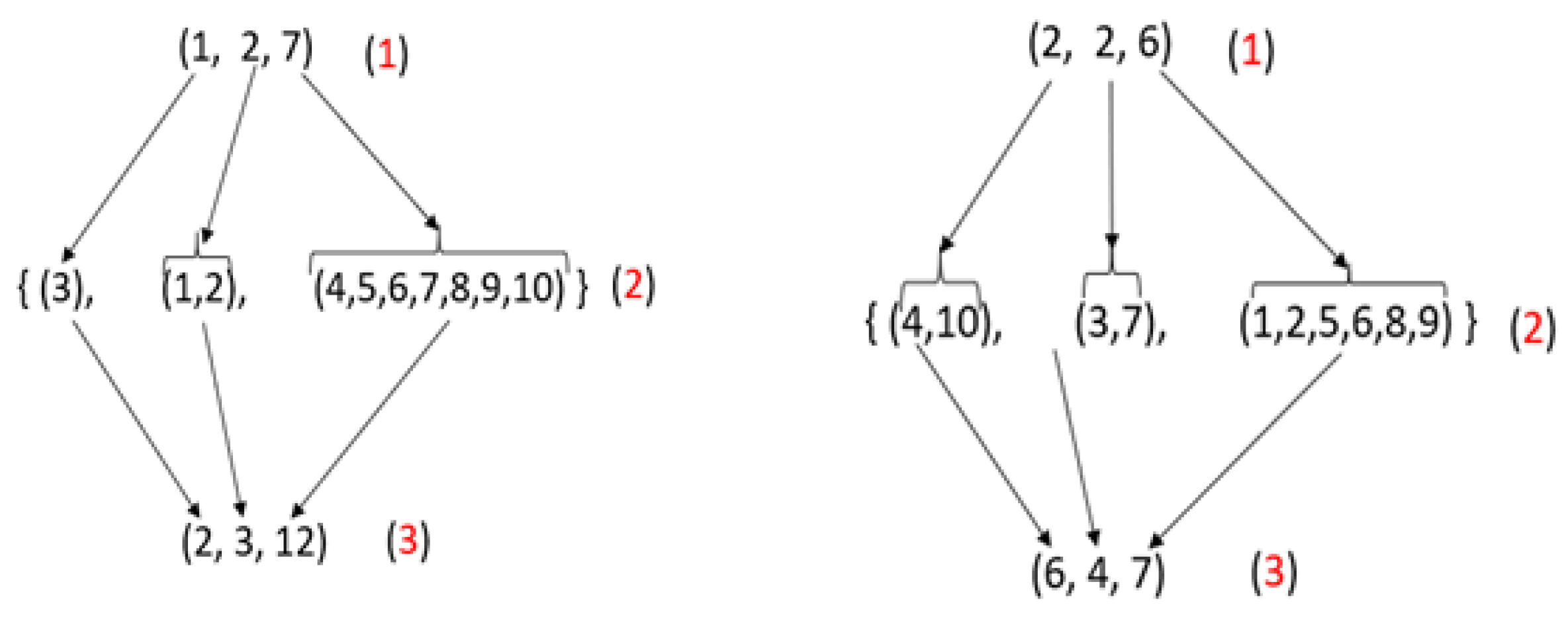
In this example, we have ten (10) resources to allocate on three (3) battlefields. The resources are heterogeneous and their values can be found in
Table 1.
We can take, as resource reference, resource no2 in green color.
Resource no1 = and so on for the others.
Creation of new strategies with the added values of the resources allocated on the same field.
Let us take two (2) strategies (1, 2, 7) and (2, 2, 6) as shown in
Figure 1 and apply the transformation rule to get new strategies:
- (1)
the number of resources allocated to the different fields
- (2)
the list of resources allocated to the fields
- (3)
adding the values of resources on the same field and finally obtaining the new strategy.
4. Comparison of Strategies
The goal of comparing strategies is to get the optimal strategy that maximizes a player’s win in a game based on that of the other player.
Let A and B be two players and N the number of fields, with a utility function U and with a utility function V respectively the strategies of players A and B. Let be the gain of player A and that of player B initially at 0.
To compare two strategies, you have to make sure that they are of the same order, that is to say that the number of battlefields is constant for both players.
If , does not change and
If , and remains unchanged
The two wins do not change in the event of a tie.
The best strategy will be the one with the biggest gain.
The strategy being defined, the next part is to propose strategies and their implementations according to the above distribution rules and using programming algorithms.
4.1. Proposed Strategies Based on Distribution Rules
Here, a number of resources have been taken into account with a finite number of battlefields. The first thing to do is to generate all the strategies, then make a simulation by comparing these different strategies, and finally highlight the most optimal. For this we have studied several proposals, each with its own rules. Each proposal resulted in the implementation of algorithms for the generation and simulation of strategies. The algorithms were coded with the JAVA programming language. The tests were done on an HP machine with the following specifications:
Model: ENVY Notebook;
Operating system: Windows 10 Family 64 bit (10.0, version 17134)
Processor: Intel® Core™ i7-7500U CPU @ 2.70 GHz (4 CPUs), 2.9 GHz;
Memory: 12,288 MB RAM or 12 Gb of RAM memory.
The following variables were used:
,
and
will mean the number of resources, the number of fields and the number of strategies generated respectively. They are used in complexities analysis in
Appendix A. There are mainly two (2) algorithms implemented in the different propositions (strategy generation algorithm and strategy simulation algorithm).
Generate all possible strategies: The first strategy proposed was to be able to generate all the possible tuples with the number of resources. A model was made in order to set up algorithms to be able to generate strategies and make simulations. The results obtained after the simulation are as follows:
- (a)
The generation of the strategies was appreciable because it did not take too long, with an acceptable algorithmic complexity in . However, the number of strategies was very high. The algorithm was very simple and fast but limited because it only took into account a number of fields less than four. Beyond three fields, the algorithm could not generate the strategies because we were faced with a problem of generalization of the algorithm, in order to take into account any given integer as a number of fields.
- (b)
The simulation consisted of making a comparison between the strategies. This comparison had a very high complexity because it depends on the number of strategies generated, and therefore, the execution time was very long.
The growth in the complexities of generation and simulation, despite having different complexities, is related to the number of resources and also the number of battlefields. That is to say that the complexity of the algorithms depends on the number of resources and that of the battlefields.
Proposition 2: Generate strategies using the partition of an integer. To drop the limit for generating strategies from the first proposal while ensuring a reduction in the execution time of the simulation, we have made modifications to obtain a new strategy that will be able to overcome the shortcomings of the first proposal. Before detailing this proposition, we will discuss a concept that was used to establish the strategies: the partition of an integer. The partition of an integer n is any increasing or decreasing sequence of non-zero integers whose sum is equal to n. It is a p-tuplet , where such as: .
The number x is the order of a partition of an integer n if the number of elements of this partition is x.
In the rest of this paper, we will focus on increasing sequences and whose elements respect the following properties for each given increasing sequence S (according to the definition of the partition of an integer):
Reflexivity: for any element ;
Transitivity: for all the elements x, y and z , if and then ;
Antisymmetry: for all the elements x and y , if and then .
With this second strategy proposal, the number of strategies generated was lower than that of the first proposal, and therefore the execution times of the different algorithms vary widely and there is a big difference between the algorithmic complexities of the two (2) propositions. However, a problem arose with this proposal, because it required players to allocate resources on all fields (at least one resource). The idea was therefore to give the choice to the players to allocate, or not, resources on a given field. In the partition of an integer it is not possible to obtain a partition with zero as an element (according to the definition). So, if our strategies respect this definition (which is the case with the second proposition), there will be no possibility for a player to not deploy resources to a given field. So we had to think about how to adopt this proposal (since it decreases the number of strategies and we have fast algorithms in execution) and to make modifications to it so that the players decide to allocate or not to allocate resources to a field that is not considered interesting for them. It is in this perspective that a third proposal was made to fill the shortcomings of this second proposal.
Proposition 3: Generate the strategies using the partition of an integer and introduce the zero:
A strategy is defined in this third proposition as a partition of an integer (resources) by forming a tuple with n the number of battlefields and including the integer zero. The partition of an integer n is defined here as any increasing sequence of integers whose sum is n. This definition has the same algebraic properties as that of the partition of a globally known integer. The only difference is that, for purposes, we introduced the integer zero to the elements of a partition. The introduction of the integer zero has a consequence because it slightly increases the number of strategies, but the execution times of the different algorithms are practically the same, with a few milliseconds of difference (sometimes the times are the same without differences). This third proposal was the last and takes into account the following properties:
Homogeneity and heterogeneity of the battlefields
Homogeneous and heterogeneous resources (type of resource)
Increasing allocation of resources
Homogeneity and heterogeneity in relation to the number of resources to be allocated
Guarantee of always having a condition of equilibrium of the game.
The last point is only guaranteed if, and only if, resources are increasingly allocated. Otherwise, it will be difficult to specify an equilibrium of the game
4.2. Assessment of the Proposed Strategy
An evaluation of the third proposal will be made here. This strategy uses several methods implemented in java and whose signatures of the different methods are given in
Appendix A. After several simulations which enabled the validation of the algorithms, a study on the complexities followed, and the results obtained are the following (the complexities are given in the worst case):
Complexity of generating all the strategies:
Complexity of combat simulation:
Consumption of the resource in terms of memory and significant execution time (especially when the number of fields exceeds three (3) and the number of resources exceeds three hundred (300)).
: the number of loop turns of the “do-while” loop
: the number of strategies generated
: the number of fields
The calculations of the complexities of the functions are detailed in the
Appendix A.
In the following section, a case study will be presented and it will be focused on the asymmetric war between an armed group and a nation.
4.3. Cases Studies
The main goal of this case study is first of all the learning of resource allocation techniques. Then, we use these learned concepts to develop a method of resource allocation with the definition of strategies to allow better decision-making. This case study will concern an asymmetric resource allocation case and is referred to as a war. This war will pit an enemy force E with an army against a nation A which also has its army. Each of the two camps tries to prepare the war well in order to win it. For this, they all have to make choices based on information they have, in order to decide which strategy to apply. Moreover, this strategy must be optimal, so as not to end up with a defeat. The strategy will consist in making a better allocation of the resources that they will deploy on the fields (in case there are several). So, this decision-making is very important and crucial, because on the one hand, there are very costly human and resource losses, and on the other hand, survival, independence etc.
Consider the following information from the side of Nation A:
The enemy has 10 colonels
Each colonel has his battalion and the maximum number of elements of each battalion is known
Enemy E occupies three (3) territories of Nation A.
A decides to face E on the 3 battlefields but it ignores the exact deployment of E on the different fields. However, to win the war, A must decide how to make a better allocation of resources in order to win all or the maximum of battles. For this, it must analyze all the scenarios, by browsing all the possible strategies of E and bring out the one that are preferred and likely to be adopted by E in terms of optimality (while taking into account the values of the occupied territories by E). So, A will proceed by a simulation on these different strategies which are likely to take days or even weeks if she has to do it by hand without using a computer program.
Suppose now that this present tool is available to nation A. So, we will apply the new strategy defined in this case study in the next section of this document.
Application of the Strategies to the Case Study
The parameters of the case study are: the resources are the colonels and they are ten (10) and the number of battlefields is three (3).
The application of the strategies to the case study will consist in generating the strategies and in making a simulation of these generated strategies. The results of the simulations will give us the numbers of times a strategy won, lost or tied against another strategy. The numbers of strategies generated with this information and considering that the resources are homogeneous are the following: (0, 0, 10), (0, 1, 9), (0, 2, 8), (0, 3, 7), (0, 4, 6), (0, 5, 5), (1, 1, 8), (1, 2, 7), (1, 3, 6), (1, 4, 5), (2, 2, 6), (2, 3, 5), (2, 4, 4), (3, 3, 4). So, we have several 3-uplet strategies for this resource allocation. There are two cases:
The 1st case is about homogeneous fields (the fields have the same value) (cf.
Figure 2). In the second case, the fields are heterogeneous (they have different values) (cf.
Figure 3).
In the two cases related to homogeneous fields, we considered that the resources are homogeneous. In the case of heterogeneous resources, we took as values of fields 1, 3 and 4. So: the value of the 1st field is 1, the value of the 2nd field is 3 and the value of the 3rd field is 4.
However, the allocation of resources is done randomly by the algorithm. So, if we have ten (10) resources with different values and a given strategy, the algorithm has to decide resources allocation, while taking into account the number to be allocated.
The 3rd case is homogeneous fields (the fields have the same value) and heterogenous resources (cf.
Figure 4) and the 4th case is related to both heterogeneous fields and heterogeneous resources (cf.
Figure 5).
The strategies that win the most by making fewer defeats and parities are the best, then come those that win less and make more parities and no or few losses and finally come those that make more losses.
4.4. Evaluation of Strategies
The definition of strategies of the previous section leads to three proposed strategies. First one that generates more strategies than the the two followings with a very fast generation algorithm and a complexity in
if the number of fields is equal to 2 or
if the number of fields is 3. In both cases, the complexity is good and is either linear or quadratic. As for the second and third propositions, they have an algorithmic complexity of
. This complexity is polynomial, and as soon as the number of resources or that of fields increases and reaches somes, the execution times of the algorithm increase (see
Table 2). The only difference between the second and the third proposition is a conditional block whose complexity is constant.
The simulation algorithms of the three propositions have the same complexity and are in
(see proof in Appendices
Appendix A and
Appendix B).
Table 2 and
Table 3 present the comparisons of different proposed strategies. The first table makes a comparison based on the algorithmic complexity of the algorithms for generating and simulating strategies; as for the second table, it will make a comparison between the results of several simulations with a some resources on some fields.
In
Table 3, we have:
nb_soldats is the number of resources,
nb is the number of fields,
nbs is the number of strategies generated, and
nbw is the number of times the
“do-while” loop does.
Evidence of these complexities is detailed in the
Appendix A.
In
Table 2, we have:
NA: Not applied. Indeed, the first proposal could not generate with a number of fields greater than 3.
The execution time is represented by a couple of values (X/Y) where X is the execution time of the generation of the strategies and Y is the execution time of the strategy simulation.
5. Conclusions
This study examined and implemented a strategic decision-making tool for resource allocation problems. Following prior works, several proposals were explored until a satisfactory proposal was obtained. Through these different proposals, we had to implement them in order to execute them to finally study the results of the different simulations. Moreover, it is at the end of each simulation that the shortcomings or limits of the proposal in question were noticed, and this allowed the development of a new strategy proposal. Finally, the strategy recently proposed was sufficient to respond to the problem posed. The strategy defined is not only applicable to the army; it can be used in several other fields (auction, elections, web advertising, allocation of resources in a service, etc.). Any area that requires resource allocation can effectively use this strategy to better allocate resources.
Table 4 shows a comparison of existing strategies and the one proposed as a solution in this project.
Furthermore, during simulations of the latter, we noted weaknesses (the non-guaranteed optimal distribution with the random allocation of resources and the significant increase in the execution times of the different algorithms) which could be taken as perspectives. A vast work deserves to be carried out by experimenting on a large scale (the use of clusters, supercomputers) the concept of resource allocation. This includes the ability to:
Propose new strategies that take into account allocating resources in an increasing or random manner, while having an acceptable algorithmic complexity and ensuring at least one condition of equilibrium.
Improve the proposed strategy and solve its problems of insufficiency.
Use parallelism or distribution mechanisms to reduce the complexity of the algorithms and thus obtain reasonable execution times.
Make the algorithm dynamic according to the situations (moves, time, difficulties).
Propose a graphical tool to facilitate the use of the algorithms implemented.
Author Contributions
Conceptualization, H.T., J.K. and O.Y.M.; methodology, O.Y.M. and J.K.; software, Y.A.K.; validation, H.T., J.K. and O.Y.M.; formal analysis, Y.A.K.; investigation, Y.A.K.; resources, H.T.; data curation, Y.A.K.; writing—original draft preparation, J.K.; writing—review and editing, H.T., O.Y.M.; supervision, J.K., O.Y.M. and H.T.; project administration, O.Y.M.; funding acquisition, J.K. All authors have read and agreed to the published version of the manuscript.
Funding
This research received no external funding.
Conflicts of Interest
The authors declare no conflict of interest.
Appendix A. Complexity Analysis of Algorithms
In the algorithms below, we used the following variables:
init: an initialization
comp: a comparison
sous: a subtraction
add: an addition
affect: an assignment
op: an operation
nb_soldats: the number of resources
nbs: the number of generated strategies
nbw: the number of iterations of the DO-WHILE loop
b: the number of battlefields
Appendix A.1. Proposition 1
Appendix A.1.1. Generating Strategies with Two Fields
The algorithm for generating strategies with two fields is shown in Code A1.
| Code A1: Generating strategies with two fields |
![Algorithms 13 00270 i001]() |
For complexity analysis, we divided the code into three parts, as follows:
- (1)
- (2)
- (3)
Finally we have:
(C1): The complexity of this algorithm is: ,
The algorithm for generating strategies with three fields is shown in Code A2.
| Code A2: Generating strategies with three fields |
![Algorithms 13 00270 i002]() |
The complexity analysis is done in nine steps, as follows:
- (1)
- (2)
- (3)
- (4)
- (5)
- (6)
- (7)
- (8)
- (9)
Finally:
We have considered that the two tables ( and ) have the same size, even if, in reality, the size of is less than that of . Since we are calculating the complexities in the worst case, we have taken the value of in (6) because the maximum value that a field can take is the total number of resources that the player has. We have with , so:
(C2): The complexity of this algorithm is:
Appendix A.1.2. Simulation of Strategies with Two and Three Fields
The algorithm for strategies simulation with two and three fields is shown by the Code A3.
| Code A3: Strategies with two and three fields simulation algorithm |
![Algorithms 13 00270 i003]() |
For complexity analysis, we divided the algorithm into seven parts, as follows:
- (1)
- (2)
- (3)
- (4)
- (5)
- (6)
- (7)
Finally, this algorithm has a complexity (C3) = .
Appendix A.2. Propositions 2 and 3
Strategies from propositions 2 and 3 have the same algorithmic complexities.
The four (04) functions used in the method that generates the strategies and their complexities are shown in the Code A, Code B, Code C and Code D.
Complexity of (A): .
Complexity of (B): .
Complexity of (C): .
Complexity of (D): .
Appendix A.2.1. Strategies Generating
The Algorithm in Code A4 is about the algorithm for generating strategies from propositions 2 and 3.
| Code A4: Calculation of the complexity of the strategy generation algorithm |
![Algorithms 13 00270 i005]() |
For complexity analysis, we divided the algorithm in 6 parts as follows:
- (1)
- (2)
- (3)
- (4)
- (5)
- (6)
Here, we are not going to consider elementary operations but we will take into account only loops and function calls in complexity calculations.
(1): =
Since , then the complexity of (1) is:
(2): It’s a simple loop so its complexity is .
(3) and (4): .
Since is greater than therefore the complexity of (3) or (4) will be in : (S1).
In (5) and (6) we have complexities of : (S2).
By applying the do-while loop to (S1) and (S2) we obtain a complexity of: where is the number of times in the do-while loop and also taking into account that . So we will have: which comes down to a complexity of .
Finally, the complexity of “” is (C4):
Appendix A.2.2. Simulation of Strategies with Homogeneous Resources
For strategies simulation from propositions 2 and 3, we are going to consider Code A5.
| Code A5: Calculation of the complexity of the strategy simulation algorithm for homogeneous resources |
![Algorithms 13 00270 i006]() |
The algorithm is divided into 3 parts for complexity analysis:
- (1)
- (2)
- (3)
The complexity of this algorithm is equal to the product of the complexities of (1), (2) and (3). So, gives a complexity of
The complexity is (C5):
Appendix A.2.3. Simulating Strategies with Heterogeneous Resources
For strategies simulation from propositions 2 and 3 we are going to consider Code A6.
| Code A6: Calculation of the complexity of the strategy simulation algorithm for heterogeneous resources |
![Algorithms 13 00270 i007]() |
To make complexity analysis, we divided the algorithm into 4 parts as follows:
- (1)
where (E)
- (2)
- (3)
- (4)
Finally, the complexity of the algorithm is as follows:
(1) + (4): =
where .
The complexity of this algorithm is (C6):
Appendix A.2.4. Generating New Strategy with Heterogeneous Resources in a Random Manner
The source code Code A7 above is the algorithm for “” method used to convert a strategy into a new strategy with the values of heterogeneous resources randomly.
| Code A7: Algorithm for strategy conversion randomly |
![Algorithms 13 00270 i008]() |
Let us consider this complexity analysis:
= : (E)
The complexity (C7): .
Appendix A.2.5. Generating Arbitrarily New Strategy with Heterogeneous Resources
The algorithm in code Code A8 does almost the same thing as that shown in Code A7. However, the first one generates strategies arbitrarily.
| Code A8: Algorithm for strategy conversion arbitrarily |
![Algorithms 13 00270 i009]() |
Here is the complexity of algorithm:
The complexity is (C8) =
Appendix B. Signature of Methods
Appendix B.1. Strategy Method
The main methods we used for strategies generating are below.
: Allows one to generate a new strategy arbitrarily using the values of the different resources given as arguments.
: Allows one to generate a new strategy randomly using the values of different resources.
: display a strategy.
: generate the strategies according to the number of resources and fields.
: checks if a generated strategy already exists in the list.
: sum of the elements of index higher than that passed in argument. : generates the key to a strategy.
: checks if the strategy is good (if it respects the allocation rules).
Appendix B.2. Resource
The method used for resources is the following.
: gives the value of a resource
Appendix B.3. Simulation
The main methods we used for strategies simulating are below.
: load strategies
: simulates with homogeneous resources, the fields can be either homogeneous or heterogeneous.
: simulates with heterogeneous resources, the fields can be either homogeneous or heterogeneous.
References
- Yildizoglu, M. Introduction à la Théorie des Jeux; ECO SUP; DUNOD: Paris, France, 2003. [Google Scholar]
- Dequiedt, V.; Durieu, J.; Solal, P. Théorie des Jeux et Applications; CorpusEconomie, 49—Rue Héricat—75015 PARIS; ECONOMICA: Bonn, Germany, 2011. [Google Scholar]
- Nash, J. Equilibrium Points in n-Person Games. Proc. Natl. Acad. Sci. USA 1950, 36, 48–49. [Google Scholar] [CrossRef] [PubMed] [Green Version]
- Edgeworth, F.Y. Mathematical Psychics; Kegan Paul: London, UK, 1881. [Google Scholar]
- Smith, J.M.; Smith, J.M.M. Evolution and the Theory of Games; Cambridge University Press: Cambridge, UK, 1982; ISBN 978-0-521-28884-2. [Google Scholar]
- Chastain, E. Algorithms, games, and evolution. Proc. Natl. Acad. Sci. USA 2014, 111, 10620–10623. [Google Scholar] [CrossRef] [PubMed] [Green Version]
- Papayoanou, P. Game Theory for Business: A Primer in Strategic Gaming; Probabilistic: Sugar Land, TX, USA, 2010; ISBN 978-0964793873. [Google Scholar]
- Shapley, L.S. Stochastic Games. Proc. Natl. Acad. Sci. USA 1953, 39, 1095–1100. [Google Scholar] [CrossRef] [PubMed]
- Tembine, H. Deep Learning Meets Game Theory: Bregman-Based Algorithms for Interactive Deep Generative Adversarial Networks. IEEE Trans. Cybern. 2020, 50, 1132–1145. [Google Scholar] [CrossRef] [PubMed]
- Khan, M.A.; Tembine, H.; Vasilakos, A.V. Game Dynamics and Cost of Learning in Heterogeneous 4G Networks. IEEE J. Sel. Areas Commun. 2012, 30, 198–213. [Google Scholar] [CrossRef]
- Tirole, J. Économie du Bien Commun; Presse Universitaire France: Paris, France, 2016. [Google Scholar]
- Tirole, J. Théorie des jeux—Une approche historique. Rapp. Tech. 1996, unpublished. [Google Scholar]
- Obin, J.-P.; Bruley, J.-L.; Colin, P.; Lagadec, I.; Le Borgne, E.; Vial, C.; Viala, J.-L. La Prise de Décision en Situation Complexe; ESENESR, 58 rue Jean-Bleuzen—CS 70007—92178 Vanves cedex; Hachette: Paris, France, 2016. [Google Scholar]
- Roberson, B. The Colonel Blotto Game; Number 1; Springer: Berlin/Heidelberg, Germany, 2006; Volume 29, pp. 1–24. [Google Scholar]
- Borel, E.; Ville, J. Application de la Théorie des Probabilités aux Jeux de Hasard; Gauthier-Villar: Paris, France, 1938. [Google Scholar]
- Roberson, B.; Kvasov, D. The Non-Constant-Sum Colonel Blotto Game; Number 2; Springer: Berlin/Heidelberg, Germany, 2012; Volume 51, pp. 397–433. [Google Scholar]
- Thomas, C. N-Dimensional Blotto Game with Heterogeneous Battlefield Values; Springer: Berlin/Heidelberg, Germany, 2017; p. 36. [Google Scholar]
- Rubinstein-Salzedo, S.; Zhu, Y. The Asymetric Colonel Blotto Game. arXiv 2017, arXiv:1708.07916v1. [Google Scholar]
| Publisher’s Note: MDPI stays neutral with regard to jurisdictional claims in published maps and institutional affiliations. |
© 2020 by the authors. Licensee MDPI, Basel, Switzerland. This article is an open access article distributed under the terms and conditions of the Creative Commons Attribution (CC BY) license (http://creativecommons.org/licenses/by/4.0/).


