A Combined Full-Reference Image Quality Assessment Method Based on Convolutional Activation Maps

Department of Networked Systems and Services, Budapest University of Technology and Economics, 1111 Budapest, Hungary
Algorithms 2020, 13(12), 313; https://doi.org/10.3390/a13120313
Submission received: 15 September 2020
/
Revised: 20 November 2020
/
Accepted: 26 November 2020
/
Published: 28 November 2020
Abstract
:The goal of full-reference image quality assessment (FR-IQA) is to predict the perceptual quality of an image as perceived by human observers using its pristine (distortion free) reference counterpart. In this study, we explore a novel, combined approach which predicts the perceptual quality of a distorted image by compiling a feature vector from convolutional activation maps. More specifically, a reference-distorted image pair is run through a pretrained convolutional neural network and the activation maps are compared with a traditional image similarity metric. Subsequently, the resulting feature vector is mapped onto perceptual quality scores with the help of a trained support vector regressor. A detailed parameter study is also presented in which the design choices of the proposed method is explained. Furthermore, we study the relationship between the amount of training images and the prediction performance. Specifically, it is demonstrated that the proposed method can be trained with a small amount of data to reach high prediction performance. Our best proposal—called ActMapFeat—is compared to the state-of-the-art on six publicly available benchmark IQA databases, such as KADID-10k, TID2013, TID2008, MDID, CSIQ, and VCL-FER. Specifically, our method is able to significantly outperform the state-of-the-art on these benchmark databases.
1. Introduction
In recent decades, a continuous growth in the number of digital images has been observed, due to the spread of smart phones and various social media. As a result of the huge number of imaging sensors, there is a massive amount of visual data being produced each day. However, digital images may suffer different distortions during the procedure of acquisition, transmission, or compression. As a result, unsatisfactory perceived visual quality or a certain level of annoyance may occur. Consequently, it is essential to predict the perceptual quality of images in many applications, such as display technology, communication, image compression, image restoration, image retrieval, object detection, or image registration. Broadly speaking, image quality assessment (IQA) algorithms can be classified into three different classes based on the availability of the reference, undistorted image. Full-reference (FR) and reduced-reference (RR) IQA algorithms have full and partial information about the reference image, respectively. In contrast, no-reference (NR) IQA methods do not posses any information about the reference image.
Convolutional neural networks (CNN), introduced by LeCun et al. [1] in 1988, are used in many applications, from image classification [2] to audio synthesis [3]. In 2012, Krizhevsky et al. [4] won the ImageNet [5] challenge by training a deep CNN relying on graphical processing units. Due to the huge number of parameters in a CNN, the training set has to contain sufficient data to avoid over-fitting. However, the number of human annotated images in many databases is rather limited to training a CNN from scratch. On the other hand, a CNN trained on ImageNet database [5] is able to provide powerful features for a wide range of image processing tasks [6,7,8], due to the learned comprehensive set of features. In this paper, we propose a combined FR-IQA metric based on the comparison of feature maps extracted from pretrained CNNs. The rest of this section is organized as follows. In Section 1.1, previous and related work are summarized and reviewed. Next, Section 1.2 outlines the main contributions of this study.
1.1. Related Work
Over the past few decades, many FR-IQA algorithms have been proposed in the literature. The earliest algorithms, such as mean squared error (MSE) and peak signal-to-noise ratio (PSNR), are based on the energy of image distortions to measure perceptual image quality. Later, methods have appeared that utilized certain characteristics of the human visual system (HVS). This kind of FR-IQA algorithms can be classified into two groups: bottom-up and top-down ones. Bottom-up approaches directly build on the properties of HVS, such as luminance adaptation [9], contrast sensitivity [10], or contrast masking [11], to create a model that enables the prediction of perceptual quality. In contrast, top-down methods try to incorporate the general characteristics of HVS into a metric to devise effective algorithms. Probably, the most famous top-down approach is the structural similarity index (SSIM) proposed by Wang et al. [12]. The main idea behind SSIM [12] is to make a distinction between structural and non-structural image distortions, because the HVS is mainly sensitive to the latter ones. Specifically, SSIM is determined at each coordinate within local windows of the distorted and the reference images. The distorted image’s overall quality is the arithmetic mean of the local windows’ values. Later, advanced forms of SSIM have been proposed. For example, edge-based structural similarity [13] (ESSIM) compares the edge information between the reference image block and the distorted one, claiming that edge information is the most important image structure information for the HVS. MS-SSIM [14] built multi-scale information to SSIM, while 3-SSIM [15] is a weighted average of different SSIMs for edges, textures, and smooth regions. Furthermore, saliency weighted [16] and information content weighted [17] SSIMs were also introduced in the literature. Feature similarity index (FSIM) [18] relies on the fact that the HVS utilizes low-level features, such as edges and zero crossings, in the early stage of visual information processing to interpret images. This is why FSIM utilizes two features: (1) phase congruency, which is a contrast-invariant dimensionless measure of the local structure and (2) an image gradient magnitude feature. Gradient magnitude similarity deviation (GMSD) [19] method utilizes the sensitivity of image gradients to image distortions and pixel-wise gradient similarity combined with a pooling strategy, applied for the prediction of the perceptual image quality. In contrast, Haar wavelet-based perceptual similarity index (HaarPSI) [20] applies coefficients obtained from Haar wavelet decomposition to compile an IQA metric. Specifically, the magnitudes of high-frequency coefficients were used to define local similarities, while the low-frequency ones were applied to weight the importance of image regions. Quaternion image processing provides a true vectorial approach to image quality assessment. Wang et al. [21] gave a quaternion description for the structural information of color images. Namely, the local variance of the luminance was taken as the real part of a quaternion, while the three RGB channels were taken as the imaginary parts of a quaternion. Moreover, the perceptual quality was characterized by the angle computed between the singular value feature vectors of the quaternion matrices derived from the distorted and the reference image. In contrast, Kolaman and Pecht [22] created a quaternion-based structural similarity index (QSSIM) to assess the quality of RGB images. A study on the effect of image features, such as contrast, blur, granularity, geometry distortion, noise, and color, on the perceived image quality can be found in [23].
Following the success in image classification [4], deep learning has become extremely popular in the field of image processing. Liang et al. [24] first introduced a dual-path convolutional neural network (CNN) containing two channels of inputs. Specifically, one input channel was dedicated to the reference image and another for the distorted image. Moreover, the presented network had one output that predicted the image quality score. First, the input distorted and reference images were decomposed into -sized image patches and the quality of each image pair was predicted independently of each other. Finally, the overall image quality was determined by averaging the scores of the image pairs. Kim and Lee [25] introduced a similar dual-path CNN but their model accepts a distorted image and an error map calculated from the reference and the distorted image as inputs. Furthermore, it generates a visual sensitivity map which is multiplied by an error map to predict perceptual image quality. Similarly to the previous algorithm, the inputs are also decomposed into smaller image patches and the overall image quality is determined by the averaging of the scores of distorted patch-error map pairs.
Recently, generic features extracted from different pretrained CNNs, such as AlexNet [4] or GoogLeNet [2], have been proven very powerful for a wide range of image processing tasks. Razavian et al. [6] applied feature vectors extracted from the OverFeat [26] network, which was trained for object classification on ImageNet ILSVRC 2013 [5], to carry out image classification, scene recognition, fine-grained recognition, attribute detection, and content-based image retrieval. The authors reported on superior results compared to those of traditional algorithms. Later, Zhang et al. [27] pointed out that feature vectors extracted from pretrained CNNs outperform traditional image quality metrics. Motivated by the above-mentioned results, a number of FR-IQA algorithms have been proposed relying on different deep features and pretrained CNNs. Amirshahi et al. [28] compared different activation maps of the reference and the distorted image extracted from AlexNet [4] CNN. Specifically, the similarity of the activation maps was measured to produce quality sub-scores. Finally, these sub-scores were aggregated to produce an overall quality value of the distorted image. In contrast, Bosse et al. [29] extracted deep features with the help of a VGG16 [30] network from reference and distorted image patches. Subsequently, the distorted and the reference deep feature vectors were fused together and mapped onto patch-wise quality scores. Finally, the patch-wise scores were pooled, supplementing with a patch weight estimation procedure to obtain the overall perceptual quality. In our previous work [31], we introduced a composition preserving deep architecture for FR-IQA relying on a Siamese layout of pretrained CNNs, feature pooling, and a feedforward neural network.
Another line of works focuses on creating combined metrics where existing FR-IQA algorithms are combined to achieve strong correlation with the subjective ground-truth scores. In [32], Okarma examined the properties of three FR-IQA metrics (MS-SSIM [14], VIF [33], and R-SVD [34]), and proposed a combined quality metric based on the arithmetical product and power of these metrics. Later, this approach was further developed using optimization techniques [35,36]. Similarly, Oszust [37] selected 16 FR-IQA metrics and applied their scores as predictor variables in a lasso regression model to obtain a combined metric. Yuan et al. [38] took a similar approach, but kernel ridge regression was utilized to fuse the scores of the IQA metrics. In contrast, Lukin et al. [39] fused the results of six metrics with the help of a neural network. Oszust [40] carried out a decision fusion based on 16 FR-IQA measures by minimizing the root mean square error of prediction performance with a genetic algorithm.
1.2. Contributions
Motivated by recent convolutional activation map based metrics [28,41], we make the following contributions in our study. Previous activation map-based approaches compared directly the similarity between reference and distorted activation maps by histogram-based similarity metrics. Subsequently, the resulted sub-scores were pooled together using different ad-hoc solutions, such as geometric mean. In contrast, we take a machine learning approach. Specifically, we compile a feature vector for each distorted-reference image pair by comparing distorted and reference activation maps with the help of traditional image similarity metrics. Subsequently, these feature vectors are mapped to perceptual quality scores using machine learning techniques. Unlike previous combined methods [35,36,39,40], we do not apply directly different optimization or machine learning techniques using the results of traditional metrics; instead, traditional metrics are used to compare convolutional activation map and to compile a feature vector.
We demonstrate that our approach has several advantages. First, the proposed FR-IQA algorithm can be easily generalized to any input image resolution or base CNN architecture, since image patches are not required to crop from the input images like several previous CNN-based approaches [24,25,29]. In this regard, it is similar to recently published NR-IQA algorithms, such as DeepFL-IQA [42] and BLINDER [43]. Second, the proposed feature extraction method is highly effective, since the proposed method is able to reach state-of-the-art results even if only 5% of the KADID-10k [44] database is used for training. In contrast, state-of-the-art deep learning based approaches’ performances are strongly dependent on the training database size [45]. Another advantage of the proposed approach is that it is able to achieve the performance of traditional FR-IQA metrics, even in cross-database tests. Our method is compared against the state-of-the-art on six publicly available IQA benchmark databases, such as KADID-10k [44], TID2013 [46], VCL-FER [47], MDID [48], CSIQ [49], and TID2008 [46]. Specifically, our method is able to significantly outperform the state-of-the-art on the benchmark databases.
1.3. Structure
The remainder of this paper is organized as follows. After this introduction, Section 2 presents our proposed approach. Section 3 shows experimental results and analysis with a parameter study, a comparison to other state-of-the-art methods, and a cross-database test. Finally, a conclusion is drawn in Section 4.
2. Proposed Method
The proposed approach is based on constructing feature vectors from each convolutional layer of a pretrained CNN for a reference-distorted image pair. Subsequently, the convolutional layer-wise feature vectors are concatenated and mapped onto perceptual quality scores with the help of a regression algorithm. In our experiments, we used the AlexNet [4] pretrained CNN which won the 2012 ILSVRC by reducing the error rate from 26.2% to 15.2%. This was the first time that a CNN performed so well on ImageNet database. The techniques, which were introduced in this model, are widely used also today, such as data augmentation and drop-out. In total, it contains five convolutional and three fully connected layers. Furthermore, rectified linear unit (ReLU) was applied after each convolutional and fully connected layer as activation function.
Architecture
In this subsection, the proposed deep FR-IQA framework, which aims to capture image features in variuous levels from a pretrained CNN, is introduced in details. Existing works extract features of one or two layers from a pretrained CNN in FR-IQA [29,31]. However, many papers pointed out the advantages of considering the features of multiple layers in NR-IQA [43] and aesthetics quality assessment [50].
We put the applied base CNN architectures into a unified framework by slicing a CNN into L parts by the convolutional layers, independent from the network architecture, e.g., AlexNet or VGG16. Without the loss of generality, the slicing of AlexNet [4] is shown in Figure 1. As one can see from Figure 1, at this point, the features are in the form of tensors, where the depth is dependent on the applied base CNN architecture and the tensors’s width and height depend on the input image size. In order to make the feature vectors’ dimension independent from the input image pairs’ resolution, we do the followings. First, convolutional feature tensors are extracted with the help of a pretrained CNN (Figure 1) from the reference image and from the corresponding distorted image. Second, reference and distorted activation maps at a given convolutional layer are compared using traditional image similarity metrics. More specifically, the ith element of a layer-wise feature vector corresponds to the similarity between the ith activation map of the reference feature tensor and ith activation map of the distorted feature tensor. Formally, we can write
where denotes a traditional image similarity metric (PSNR, SSIM [12], and HaarPSI [20] are considered in this study), and are the ith activation map from the lth reference and distorted feature tensors, is the feature vector extracted from the lth convolutional layer, and stands for its ith element. Figure 2 illustrates the compilation of layer-wise feature vectors.
In contrast to other machine learning techniques, CNNs are often called black-box techniques due to millions of parameters and highly nonlinear internal representations of the data. Activation maps of an input image help us to understand which features that a CNN has learned. If we feed AlexNet reference and distorted image pairs and we visualize the activations of the conv1 layer, it can be seen that activations of the reference image and those of the distorted image differs significantly from each other mainly in quality aware details, such as edges and textures (see Figure 3 and Figure 4 for illustration). This observation revealed to us that an effective feature vector can be compiled by comparing the activation maps.
The whole feature vector, that characterizes a reference-distorted image pair, can be obtained by concatenating the layer-wise feature vectors. Formally, we can write
where stands for the whole feature vector, is the jth layer-wise feature vector, and L denotes the number of convolutional layers in the applied base CNN.
Finally, a regression algorithm is applied to map the feature vectors onto perceptual quality scores. In this study, we made experiments with two different regression techniques, such as support vector regressor (SVR) [51] and Gaussian process regressor (GPR) [52]. Specifically, we applied SVR with linear kernel and radial basis function (RBF) kernel. GPR was applied with rational quadratic kernel.
3. Experimental Results
In this section, we present our experimental results and analysis. First, we introduce the applied evaluation metrics in Section 3.1. Second, the implementation details and the experimental setup are given in Section 3.2. Subsequently, a detailed parameter study is presented in Section 3.3, in which we extensively reason the design choices of our proposed method. In Section 3.4, we explore the performance of our proposed method on different distortion types and distortion intensity levels. Subsequently, we examine the relationship between the performance and the amount of training data in Section 3.5. In Section 3.6, a comparison to other state-of-the-art method is carried out using six benchmark IQA databases, such as KADID-10k [44], TID2013 [53], TID2008 [46], VCL-FER [47], CSIQ [49], and MDID [48]. The results of the cross database are presented in Section 3.7. Table 1 illustrates some facts about the publicly available IQA databases used in this paper. It allows comparisons between the number of reference and test images, image resolutions, the number of distortion levels, and the number of distortion types.
3.1. Evaluation Metrics
A reliable way to evaluate objective FR-IQA methods is based on measuring the correlation strength between the ground-truth scores of a publicly available IQA database and the predicted scores. In the literature, Pearson’s linear correlation coefficient (PLCC), Spearman’s rank-order correlation coefficient (SROCC), and Kendall’s rank-order correlation coefficient (KROCC) are widely applied to characterize the degree of correlation. PLCC between vectors x and y can be expressed as
where and . Furthermore, x stands for the vector containing the ground-truth scores, while y vector consists of the predicted scores. PLCC performance indices are determined after a non-linear mapping between objective scores (MOS or differential MOS values) and predicted subjective scores using a 5-parameter logistic function, as recommended by the authors of [54].
SROCC between vectors x and y can be defined as
where the function gives back a vector whose ith element is the rank of the ith element in the input vector. As a consequence, SROCC between vectors x and y can also be expressed as
where and stand for the middle ranks of and , respectively.
KROCC between vectors x and y can be determined as
where n is the length of the input vectors, stands for the number of concordant pairs between and , and denotes the number of discordant pairs.
3.2. Experimental Setup
KADID-10k [44] was used to carry out a detailed parameter study to determine the best design choices of the proposed method. Subsequently, other publicly available databases, such as TID2013 [53], TID2008 [46], VCL-FER [47], CSIQ [49], and MDID [48], were also applied to carry out a comparison to other state-of-the-art FR-IQA algorithms. Furthermore, our algorithms and other learning-based state-of-the-art methods were evaluated by 5-fold cross-validation with 100 repetitions. Specifically, an IQA database was divided randomly into a training set (appx. 80%) and a test set (appx. 20%) with respect to the reference, pristine images. As a consequence, there was no semantic content overlapping between these sets. Moreover, we report on the average PLCC, SROCC, and KROCC values.
All models were implemented and tested in MATLAB R2019a, relying mainly on the functions of the Deep Learning Toolbox (formerly Neural Network Toolbox), Statistics and Machine Learning Toolbox, and the Image Processing Toolbox.
3.3. Parameter Study
In this subsection, we present a detailed parameter study using the publicly available KADID-10k [44] database to find the optimal design choices of our proposed method. Specifically, we compared the performance of three traditional metrics (PSNR, SSIM [12], and HaarPSI [20]). Furthermore, we compared the performance of three different regression algorithms, such as linear SVR, Gaussian SVR, and GPR with rational quadratic kernel function. As already mentioned, the evaluation is based on 100 random train-test splits. Moreover, mean PLCC, SROCC, and KROCC values are reported. The results of the parameter study are summarized in Figure 5. From these results, it can be seen that HaarPSI metric with Gaussian SVR provides the best results. This architecture is called ActMapFeat in the further sections.
3.4. Performance over Different Distortion Types and Levels
In this subsection, we examine the performance of the proposed ActMapFeat over different image distortion types and levels of KADID-10k [44]. Namely, KADID-10k consists of images with 25 distortion types in 5 levels. Furthermore, the distortion types can be classified into five groups: blurs, color distortions, compression, noise, brightness change, spatial distortions, and sharpness and contrast.
The reported mean PLCC, SROCC, and KROCC values were measured over 100 random train-test splits in Table 2. From these results, it can be observed that ActMapFeat is able to perform relatively uniformly over different image distortion types with the exception of some color- (color shift, color saturation 1.), brightness- (mean shift), and patch-related (non-eccentricity patch. color block) noise types. Furthermore, it performs very well on different blur (Gaussian blur, lens blur, motion blur) and compression types (JPEG, JPEG2000).
The performance results of ActMapFeat over different distortion levels of KADID-10k [44] are illustrated in Table 3. From these results, it can be observed that the proposed method performs relatively uniformly over the different distortion levels. Specifically, it achieves better results on higher distortion levels than on lower ones. Moreover, the best results can be experienced at moderate distortion levels.
3.5. Effect of the Training Set Size
In general, the number of training images has a strong impact on the performance of machine/deep learning systems [44,45,55]. In this subsection, we study the relationship between the number of training images and the performance using the KADID-10k [44] database. In our experiments, the ratio of the training images in the database varied from 5% to 80%, while at the same time, those of the test images varied from 95% to 20%. The results are illustrated in Figure 6. It can be observed that the proposed system is rather robust to the size of the training set. Specifically, the mean PLCC, SROCC, and KROCC are , , and , if the ratio of the training images is 5%. These performance metrics increase to , , and , respectively, when the ratio of the training set reaches 80%, which is a common choice in machine learning. On the whole, our system can be trained with few amount of data to reach relatively high PLCC, SROCC, and KROCC values. This proves the effectiveness of the proposed feature extraction method from distorted reference image pairs.
3.6. Comparison to the State-of-the-Art
Our proposed algorithm was compared to several state-of-the-art FR-IQA metrics, including SSIM [12], MS-SSIM [14], MAD [49], GSM [56], HaarPSI [20], MDSI [57], CSV [58], GMSD [19], DSS [59], VSI [60], PerSIM [61], BLeSS-SR-SIM [62], BLeSS-FSIM [62], BLeSS-FSIMc [62], LCSIM1 [40], ReSIFT [63], IQ() [28], MS-UNIQUE [64], RVSIM [65], 2stepQA [66], SUMMER [67], CEQI [68], CEQIc [68], VCGS [69], and DISTS [70], whose original source code are available online. Moreover, we reimplemented SSIM CNN [41] in MATLAB R2019a (Available: https://github.com/Skythianos/SSIM-CNN). For learning-based approaches, we retrained the models using exactly the same database partition (approx. 80% for training and 20% for testing with respect to the reference images to avoid semantic overlap) that we used for our method. Since the feature extraction part of LCSIM1 [40] was not given, we can report the results of LCSIM1 on TID2013 [53], CSIQ [49], and TID2008 [46] databases. Furthermore, mean PLCC, SROCC, and KROCC values were measured over 100 random train-test splits for machine learning-based algorithms. In contrast, traditional FR-IQA metrics are tested on the whole database, and we report on the PLCC, SROCC, and KROCC values. Besides FR-IQA methods, some recently published deep learning-based NR-IQA algorithms, including DeepFL-IQA [42], BLINDER [43], RankIQA [71], BPSOM-MD [72], and NSSADNN [73], have been added to our comparison. Due to the difficulty of reimplementation of deep NR-IQA methods, the performance numbers in the corresponding papers are reported in this study.
The results of the performance comparison to the state-of-the-art on KADID-10k [44], TID2013 [53], VCL-FER [47], TID2008 [46], MDID [48], and CSIQ [49] are summarized in Table 4, Table 5 and Table 6, respectively. It can be observed that the performance of the examined state-of-the-art FR-IQA algorithms are far from perfect on KADID-10k [44]. In contrast, our method was able to produce PLCC and SROCC values over 0.95. Furthermore, our KROCC value is about 0.09 higher than the second the best one. On the smaller TID2013 [53], TID2008 [46], MDID [48], and VCL-FER [47] IQA databases, the performances of the examined state-of-the-art approaches significantly improve. In spite of this, our method also gives the best results on these databases in terms of PLCC, SROCC, and KROCC, as well. Similarly, our method achieves the best results on CSIQ [49]. On the other hand, the difference between the proposed method and other state-of-the-art methods is observably less than those on the other IQA benchmark databases. Significance tests were also carried out to prove that the achieved improvements on benchmark data sets are significant. More precisely, the ITU (International Telecommunication Union) guidelines [74] for evaluating quality models were followed. The hypothesis for a given correlation coefficient (PLCC, SROCC, or KROCC) was that a rival state-of-the-art method produces not significantly different values with . Moreover, the variances of the z-transforms were determined as , where N stands for the number of images in a given IQA database. In Table 4, Table 5 and Table 6, the green background color stands for the fact that the correlation is lower than those of the proposed method and the difference is statistically.
Figure 7 depicts scatter plots of ground-truth MOS values against predicted MOS values on MDID [48], TID2008 [46], TID2013 [53], VCL-FER [47], KADID-10k [44], and CSIQ [49] test sets. Figure 8 depicts the box plots of the measured PLCC, SROCC, and KROCC values over 100 random train-test splits. On each box, the central mark denotes the median, and the bottom and top edges of the box represent the 25th and 75th percentiles, respectively. Moreover, the whiskers extend to the most extreme values which are not considered outliers.
3.7. Cross Database Test
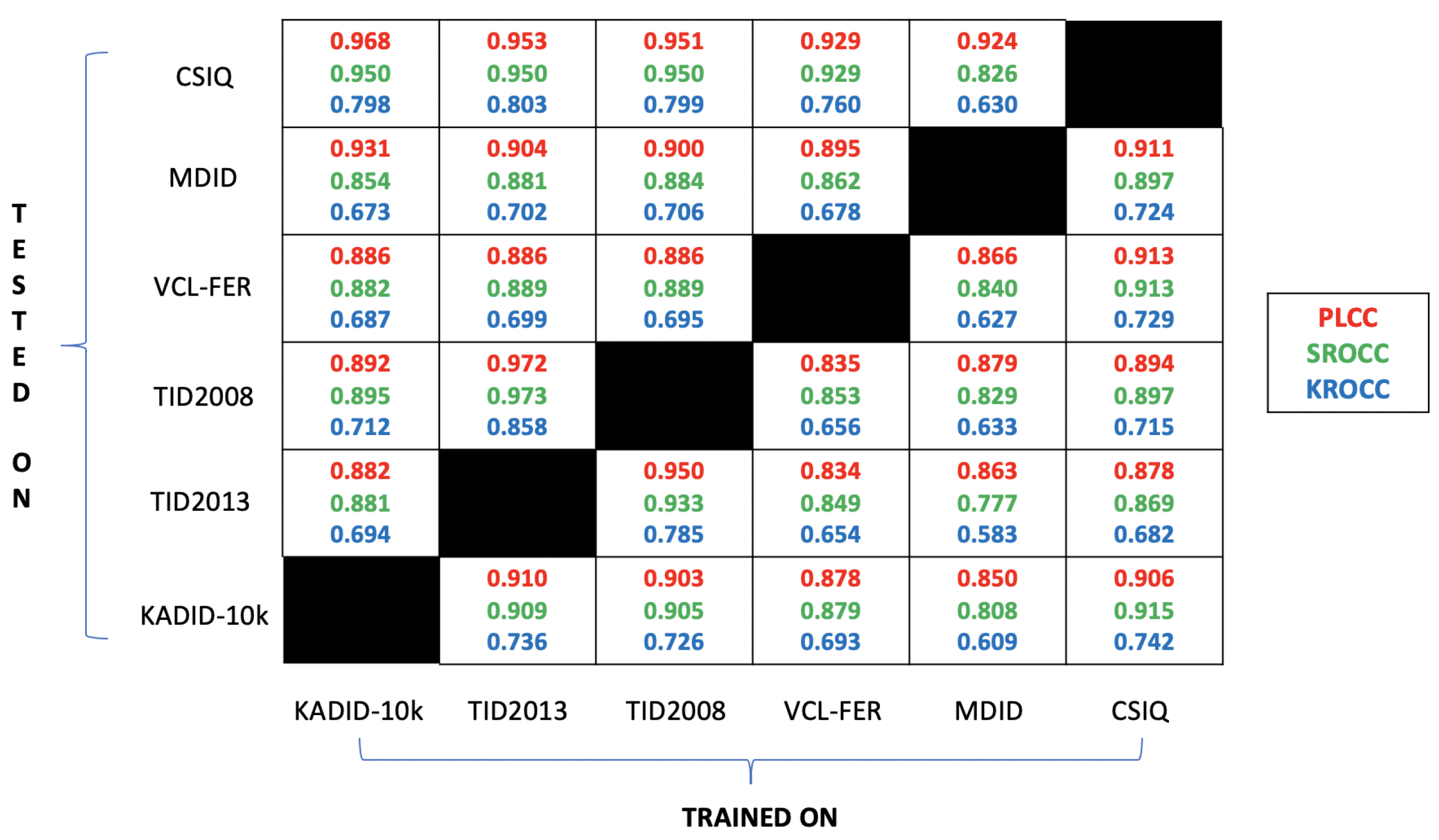
Cross database test refers to the procedure of training on one given IQA benchmark database and testing on another to show the generalization potential of a machine learning based method. The results of the cross database test using KADID-10k [44], TID2013 [53], TID2008 [46], VCL-FER [47], MDID [48], and CSIQ [49] are depicted in Figure 9. From these results, it can be concluded that the proposed method loses from its performance significantly in most cases, but is still able to achieve the performance of traditional state-of-the-art FR-IQA metrics. Moreover, there are some pairings, such as trained on KADID-10k [44] and tested on CSIQ [49], trained on TID2013 [53] and tested on TID2008 [46], trained on TID2008 [46] and tested on TID2013 [53], where the performance loss is rather minor.
4. Conclusions
In this paper, we introduced a framework for FR-IQA relying on feature vectors, which were obtained by comparing reference and distorted activation maps by traditional image similarity metrics. Unlike previous CNN-based approaches, our method does not take patches from the distorted-reference image pairs, but instead obtains convolutional activation maps and creates feature vectors from these maps. This way, our method can be easily generalized to any input image resolutions or base CNN architecture. Furthermore, we carried out a detailed parameter study with respect to the applied regression technique and image similarity metric. Moreover, we pointed out that the proposed feature extraction method is effective, since our method is able to reach high PLCC, SROCC, and KROCC values trained only on 5% of KADID-10k images. Our algorithm was compared to 26 other state-of-the-art FR-IQA methods on six benchmark IQA databases, such as KADID-10k, TID2013, VCL-FER, MDID, TID2008, and CSIQ. Our method was able to outperform the state-of-the-art in terms of PLCC, SROCC, and KROCC, as well. The generalization ability of the proposed method was confirmed in cross database tests.
To facilitate the reproducibility of the presented results, the MATLAB source code of the introduced method and test environments is available at https://github.com/Skythianos/FRIQA-ActMapFeat.
Funding
This research received no external funding.
Acknowledgments
The author thanks the anonymous reviewers for their careful reading of the manuscript and their many insightful comments and suggestions.
Conflicts of Interest
The author declares no conflict of interest.
References
- LeCun, Y.; Bottou, L.; Bengio, Y.; Haffner, P. Gradient-based learning applied to document recognition. Proc. IEEE 1998, 86, 2278–2324. [Google Scholar] [CrossRef] [Green Version]
- Szegedy, C.; Liu, W.; Jia, Y.; Sermanet, P.; Reed, S.; Anguelov, D.; Erhan, D.; Vanhoucke, V.; Rabinovich, A. Going deeper with convolutions. In Proceedings of the IEEE Conference on Computer Vision and Pattern Recognition, Boston, MA, USA, 7–12 June 2015; pp. 1–9. [Google Scholar]
- Oord, A.v.d.; Dieleman, S.; Zen, H.; Simonyan, K.; Vinyals, O.; Graves, A.; Kalchbrenner, N.; Senior, A.; Kavukcuoglu, K. Wavenet: A generative model for raw audio. arXiv 2016, arXiv:1609.03499. [Google Scholar]
- Krizhevsky, A.; Sutskever, I.; Hinton, G.E. Imagenet classification with deep convolutional neural networks. In Proceedings of the Advances in Neural Information Processing Systems, Lake Tahoe, NV, USA, 3–6 December 2012; pp. 1097–1105. [Google Scholar]
- Russakovsky, O.; Deng, J.; Su, H.; Krause, J.; Satheesh, S.; Ma, S.; Huang, Z.; Karpathy, A.; Khosla, A.; Bernstein, M.; et al. Imagenet large scale visual recognition challenge. Int. J. Comput. Vis. 2015, 115, 211–252. [Google Scholar] [CrossRef] [Green Version]
- Sharif Razavian, A.; Azizpour, H.; Sullivan, J.; Carlsson, S. CNN features off-the-shelf: An astounding baseline for recognition. In Proceedings of the IEEE Conference on Computer Vision and Pattern Recognition Workshops; IEEE Computer Society: Washington, DC, USA, 2014; pp. 806–813. [Google Scholar]
- Penatti, O.A.; Nogueira, K.; Dos Santos, J.A. Do deep features generalize from everyday objects to remote sensing and aerial scenes domains? In Proceedings of the IEEE Conference on Computer Vision and Pattern Recognition Workshops, Boston, MA, USA, 7–12 June 2015; pp. 44–51. [Google Scholar]
- Bousetouane, F.; Morris, B. Off-the-shelf CNN features for fine-grained classification of vessels in a maritime environment. In International Symposium on Visual Computing; Springer: Berlin/Heidelberg, Germany, 2015; pp. 379–388. [Google Scholar]
- Chou, C.H.; Li, Y.C. A perceptually tuned subband image coder based on the measure of just-noticeable-distortion profile. IEEE Trans. Circuits Syst. Video Technol. 1995, 5, 467–476. [Google Scholar] [CrossRef]
- Daly, S.J. Visible differences predictor: An algorithm for the assessment of image fidelity. In Human Vision, Visual Processing, and Digital Display III. International Society for Optics and Photonics; SPIE: Bellingham, WA, USA, 1992; Volume 1666, pp. 2–15. [Google Scholar]
- Watson, A.B.; Borthwick, R.; Taylor, M. Image quality and entropy masking. In Human Vision and Electronic Imaging II. International Society for Optics and Photonics; SPIE: Bellingham, WA, USA, 1997; Volume 3016, pp. 2–12. [Google Scholar]
- Wang, Z.; Bovik, A.C.; Sheikh, H.R.; Simoncelli, E.P. Image quality assessment: From error visibility to structural similarity. IEEE Trans. Image Process. 2004, 13, 600–612. [Google Scholar] [CrossRef] [Green Version]
- Chen, G.H.; Yang, C.L.; Po, L.M.; Xie, S.L. Edge-based structural similarity for image quality assessment. In Proceedings of the 2006 IEEE International Conference on Acoustics Speech and Signal Processing Proceedings, Toulouse, France, 14–19 May 2006; Volume 2, p. II. [Google Scholar]
- Wang, Z.; Simoncelli, E.P.; Bovik, A.C. Multiscale structural similarity for image quality assessment. In Proceedings of the Thrity-Seventh Asilomar Conference on Signals, Systems & Computers, Pacific Grove, CA, USA, 9–12 November 2003; Volume 2, pp. 1398–1402. [Google Scholar]
- Li, C.; Bovik, A.C. Three-component weighted structural similarity index. In Proceedings of the Image Quality and System Performance VI, International Society for Optics and Photonics, San Jose, CA, USA, 19–21 January 2009; Volume 7242, p. 72420Q. [Google Scholar]
- Liu, H.; Heynderickx, I. Visual attention in objective image quality assessment: Based on eye-tracking data. IEEE Trans. Circuits Syst. Video Technol. 2011, 21, 971–982. [Google Scholar]
- Wang, Z.; Li, Q. Information content weighting for perceptual image quality assessment. IEEE Trans. Image Process. 2010, 20, 1185–1198. [Google Scholar] [CrossRef]
- Zhang, L.; Zhang, L.; Mou, X.; Zhang, D. FSIM: A feature similarity index for image quality assessment. IEEE Trans. Image Process. 2011, 20, 2378–2386. [Google Scholar] [CrossRef] [Green Version]
- Xue, W.; Zhang, L.; Mou, X.; Bovik, A.C. Gradient magnitude similarity deviation: A highly efficient perceptual image quality index. IEEE Trans. Image Process. 2013, 23, 684–695. [Google Scholar] [CrossRef] [Green Version]
- Reisenhofer, R.; Bosse, S.; Kutyniok, G.; Wiegand, T. A Haar wavelet-based perceptual similarity index for image quality assessment. Signal Process. Image Commun. 2018, 61, 33–43. [Google Scholar] [CrossRef] [Green Version]
- Wang, Y.; Liu, W.; Wang, Y. Color image quality assessment based on quaternion singular value decomposition. In Proceedings of the 2008 Congress on Image and Signal Processing, Sanya, China, 27–30 May 2008; Volume 3, pp. 433–439. [Google Scholar]
- Kolaman, A.; Yadid-Pecht, O. Quaternion structural similarity: A new quality index for color images. IEEE Trans. Image Process. 2011, 21, 1526–1536. [Google Scholar] [CrossRef] [PubMed]
- Głowacz, A.; Grega, M.; Gwiazda, P.; Janowski, L.; Leszczuk, M.; Romaniak, P.; Romano, S.P. Automated qualitative assessment of multi-modal distortions in digital images based on GLZ. Ann. Telecommun. 2010, 65, 3–17. [Google Scholar] [CrossRef]
- Liang, Y.; Wang, J.; Wan, X.; Gong, Y.; Zheng, N. Image quality assessment using similar scene as reference. In European Conference on Computer Vision; Springer: Berlin/Heidelberg, Germany, 2016; pp. 3–18. [Google Scholar]
- Kim, J.; Lee, S. Deep learning of human visual sensitivity in image quality assessment framework. In Proceedings of the IEEE Conference on Computer Vision and Pattern Recognition, Honolulu, HI, USA, 21–26 July 2017; pp. 1676–1684. [Google Scholar]
- Sermanet, P.; Eigen, D.; Zhang, X.; Mathieu, M.; Fergus, R.; LeCun, Y. Overfeat: Integrated recognition, localization and detection using convolutional networks. arXiv 2013, arXiv:1312.6229. [Google Scholar]
- Zhang, R.; Isola, P.; Efros, A.A.; Shechtman, E.; Wang, O. The unreasonable effectiveness of deep features as a perceptual metric. In Proceedings of the IEEE Conference on Computer Vision and Pattern Recognition, Salt Lake City, UT, USA, 18–23 June 2018; pp. 586–595. [Google Scholar]
- Ali Amirshahi, S.; Pedersen, M.; Yu, S.X. Image quality assessment by comparing cnn features between images. Electron. Imaging 2017, 2017, 42–51. [Google Scholar] [CrossRef] [Green Version]
- Bosse, S.; Maniry, D.; Müller, K.R.; Wiegand, T.; Samek, W. Deep neural networks for no-reference and full-reference image quality assessment. IEEE Trans. Image Process. 2017, 27, 206–219. [Google Scholar] [CrossRef] [PubMed] [Green Version]
- Simonyan, K.; Zisserman, A. Very deep convolutional networks for large-scale image recognition. arXiv 2014, arXiv:1409.1556. [Google Scholar]
- Varga, D. Composition-preserving deep approach to full-reference image quality assessment. Signal Image Video Process. 2020, 14, 1265–1272. [Google Scholar] [CrossRef]
- Okarma, K. Combined full-reference image quality metric linearly correlated with subjective assessment. In International Conference on Artificial Intelligence and Soft Computing; Springer: Berlin/Heidelberg, Germany, 2010; pp. 539–546. [Google Scholar]
- Sheikh, H.R.; Bovik, A.C. Image information and visual quality. IEEE Trans. Image Process. 2006, 15, 430–444. [Google Scholar] [CrossRef]
- Mansouri, A.; Aznaveh, A.M.; Torkamani-Azar, F.; Jahanshahi, J.A. Image quality assessment using the singular value decomposition theorem. Opt. Rev. 2009, 16, 49–53. [Google Scholar] [CrossRef]
- Okarma, K. Combined image similarity index. Opt. Rev. 2012, 19, 349–354. [Google Scholar] [CrossRef]
- Okarma, K. Extended hybrid image similarity–combined full-reference image quality metric linearly correlated with subjective scores. Elektron. Elektrotechnika 2013, 19, 129–132. [Google Scholar] [CrossRef] [Green Version]
- Oszust, M. Image quality assessment with lasso regression and pairwise score differences. Multimed. Tools Appl. 2017, 76, 13255–13270. [Google Scholar] [CrossRef] [Green Version]
- Yuan, Y.; Guo, Q.; Lu, X. Image quality assessment: A sparse learning way. Neurocomputing 2015, 159, 227–241. [Google Scholar] [CrossRef]
- Lukin, V.V.; Ponomarenko, N.N.; Ieremeiev, O.I.; Egiazarian, K.O.; Astola, J. Combining full-reference image visual quality metrics by neural network. In Human Vision and Electronic Imaging XX; International Society for Optics and Photonics: San Diego, CA, USA, 2015; Volume 9394, p. 93940K. [Google Scholar]
- Oszust, M. Full-reference image quality assessment with linear combination of genetically selected quality measures. PLoS ONE 2016, 11, e0158333. [Google Scholar] [CrossRef] [Green Version]
- Amirshahi, S.A.; Pedersen, M.; Beghdadi, A. Reviving Traditional Image Quality Metrics Using CNNs. In Proceedings of the Color and Imaging Conference, Society for Imaging Science and Technology, Vancouver, BC, Canada, 12–16 November 2018; Volume 2018, pp. 241–246. [Google Scholar]
- Lin, H.; Hosu, V.; Saupe, D. DeepFL-IQA: Weak Supervision for Deep IQA Feature Learning. arXiv 2020, arXiv:2001.08113. [Google Scholar]
- Gao, F.; Yu, J.; Zhu, S.; Huang, Q.; Tian, Q. Blind image quality prediction by exploiting multi-level deep representations. Pattern Recognit. 2018, 81, 432–442. [Google Scholar] [CrossRef]
- Lin, H.; Hosu, V.; Saupe, D. KADID-10k: A Large-scale Artificially Distorted IQA Database. In Proceedings of the 2019 Eleventh International Conference on Quality of Multimedia Experience (QoMEX), Berlin, Germany, 5–7 June 2019; pp. 1–3. [Google Scholar]
- Lin, H.; Hosu, V.; Saupe, D. KonIQ-10K: Towards an ecologically valid and large-scale IQA database. arXiv 2018, arXiv:1803.08489. [Google Scholar]
- Ponomarenko, N.; Lukin, V.; Zelensky, A.; Egiazarian, K.; Carli, M.; Battisti, F. TID2008-a database for evaluation of full-reference visual quality assessment metrics. Adv. Mod. Radioelectron. 2009, 10, 30–45. [Google Scholar]
- Zarić, A.; Tatalović, N.; Brajković, N.; Hlevnjak, H.; Lončarić, M.; Dumić, E.; Grgić, S. VCL@ FER image quality assessment database. AUTOMATIKA Časopis Autom. Mjer. Elektron. Računarstvo Komun. 2012, 53, 344–354. [Google Scholar] [CrossRef]
- Sun, W.; Zhou, F.; Liao, Q. MDID: A multiply distorted image database for image quality assessment. Pattern Recognit. 2017, 61, 153–168. [Google Scholar] [CrossRef]
- Larson, E.C.; Chandler, D.M. Most apparent distortion: Full-reference image quality assessment and the role of strategy. J. Electron. Imaging 2010, 19, 011006. [Google Scholar]
- Hii, Y.L.; See, J.; Kairanbay, M.; Wong, L.K. Multigap: Multi-pooled inception network with text augmentation for aesthetic prediction of photographs. In Proceedings of the 2017 IEEE International Conference on Image Processing (ICIP), Beijing, China, 17–20 September 2017; pp. 1722–1726. [Google Scholar]
- Drucker, H.; Burges, C.J.; Kaufman, L.; Smola, A.J.; Vapnik, V. Support vector regression machines. In Advances in Neural Information Processing Systems; MIT Press: Cambridge, MA, USA, 1997; pp. 155–161. [Google Scholar]
- Williams, C.K.; Rasmussen, C.E. Gaussian Processes for Machine Learning; MIT Press: Cambridge, MA, USA, 2006; Volume 2. [Google Scholar]
- Ponomarenko, N.; Jin, L.; Ieremeiev, O.; Lukin, V.; Egiazarian, K.; Astola, J.; Vozel, B.; Chehdi, K.; Carli, M.; Battisti, F.; et al. Image database TID2013: Peculiarities, results and perspectives. Signal Process. Image Commun. 2015, 30, 57–77. [Google Scholar] [CrossRef] [Green Version]
- Sheikh, H.R.; Sabir, M.F.; Bovik, A.C. A statistical evaluation of recent full reference image quality assessment algorithms. IEEE Trans. Image Process. 2006, 15, 3440–3451. [Google Scholar] [CrossRef] [PubMed]
- Cho, J.; Lee, K.; Shin, E.; Choy, G.; Do, S. How much data is needed to train a medical image deep learning system to achieve necessary high accuracy? arXiv 2015, arXiv:1511.06348. [Google Scholar]
- Liu, A.; Lin, W.; Narwaria, M. Image quality assessment based on gradient similarity. IEEE Trans. Image Process. 2011, 21, 1500–1512. [Google Scholar]
- Nafchi, H.Z.; Shahkolaei, A.; Hedjam, R.; Cheriet, M. Mean deviation similarity index: Efficient and reliable full-reference image quality evaluator. IEEE Access 2016, 4, 5579–5590. [Google Scholar] [CrossRef]
- Temel, D.; AlRegib, G. CSV: Image quality assessment based on color, structure, and visual system. Signal Process. Image Commun. 2016, 48, 92–103. [Google Scholar] [CrossRef] [Green Version]
- Balanov, A.; Schwartz, A.; Moshe, Y.; Peleg, N. Image quality assessment based on DCT subband similarity. In Proceedings of the 2015 IEEE International Conference on Image Processing (ICIP), Quebec City, QC, Canada, 27–30 September 2015; pp. 2105–2109. [Google Scholar]
- Zhang, L.; Shen, Y.; Li, H. VSI: A visual saliency-induced index for perceptual image quality assessment. IEEE Trans. Image Process. 2014, 23, 4270–4281. [Google Scholar] [CrossRef] [Green Version]
- Temel, D.; AlRegib, G. PerSIM: Multi-resolution image quality assessment in the perceptually uniform color domain. In Proceedings of the 2015 IEEE International Conference on Image Processing (ICIP), Quebec City, QC, Canada, 27–30 September 2015; pp. 1682–1686. [Google Scholar]
- Temel, D.; AlRegib, G. BLeSS: Bio-inspired low-level spatiochromatic similarity assisted image quality assessment. In Proceedings of the 2016 IEEE International Conference on Multimedia and Expo (ICME), Seattle, WA, USA, 11–15 July 2016; pp. 1–6. [Google Scholar]
- Temel, D.; AlRegib, G. ReSIFT: Reliability-weighted sift-based image quality assessment. In Proceedings of the 2016 IEEE International Conference on Image Processing (ICIP), Phoenix, AZ, USA, 25–28 September 2016; pp. 2047–2051. [Google Scholar]
- Prabhushankar, M.; Temel, D.; AlRegib, G. Ms-unique: Multi-model and sharpness-weighted unsupervised image quality estimation. Electron. Imaging 2017, 2017, 30–35. [Google Scholar] [CrossRef] [Green Version]
- Yang, G.; Li, D.; Lu, F.; Liao, Y.; Yang, W. RVSIM: A feature similarity method for full-reference image quality assessment. EURASIP J. Image Video Process. 2018, 2018, 6. [Google Scholar] [CrossRef] [Green Version]
- Yu, X.; Bampis, C.G.; Gupta, P.; Bovik, A.C. Predicting the quality of images compressed after distortion in two steps. IEEE Trans. Image Process. 2019, 28, 5757–5770. [Google Scholar] [CrossRef] [PubMed]
- Temel, D.; AlRegib, G. Perceptual image quality assessment through spectral analysis of error representations. Signal Process. Image Commun. 2019, 70, 37–46. [Google Scholar] [CrossRef] [Green Version]
- Layek, M.; Uddin, A.; Le, T.P.; Chung, T.; Huh, E.-N. Center-emphasized visual saliency and a contrast-based full reference image quality index. Symmetry 2019, 11, 296. [Google Scholar] [CrossRef] [Green Version]
- Shi, C.; Lin, Y. Full Reference Image Quality Assessment Based on Visual Salience with Color Appearance and Gradient Similarity. IEEE Access 2020. [Google Scholar] [CrossRef]
- Ding, K.; Ma, K.; Wang, S.; Simoncelli, E.P. Image quality assessment: Unifying structure and texture similarity. arXiv 2020, arXiv:2004.07728. [Google Scholar]
- Liu, X.; van de Weijer, J.; Bagdanov, A.D. Rankiqa: Learning from rankings for no-reference image quality assessment. In Proceedings of the IEEE International Conference on Computer Vision, Venice, Italy, 22–29 October 2017; pp. 1040–1049. [Google Scholar]
- Pan, D.; Shi, P.; Hou, M.; Ying, Z.; Fu, S.; Zhang, Y. Blind predicting similar quality map for image quality assessment. In Proceedings of the IEEE Conference on Computer Vision and Pattern Recognition, Salt Lake City, UT, USA, 18–23 June 2018; pp. 6373–6382. [Google Scholar]
- Yan, B.; Bare, B.; Tan, W. Naturalness-aware deep no-reference image quality assessment. IEEE Trans. Multimed. 2019, 21, 2603–2615. [Google Scholar] [CrossRef]
- ITU-T. P.1401: Methods, Metrics and Procedures for Statistical Evaluation, Qualification and Comparison of Objective Quality Prediction Models. 2012. Available online: https://www.itu.int/rec/T-REC-P.1401-202001-I/en (accessed on 13 January 2020).
Figure 1.
Feature extraction with the help of AlexNet [4].
Figure 1.
Feature extraction with the help of AlexNet [4].

Figure 2.
Compilation of layer-wise feature vectors. The activation maps of a distorted-reference image pair are compared to each other in a given convolutional layer with the help of traditional image similarity metrics (SM).
Figure 2.
Compilation of layer-wise feature vectors. The activation maps of a distorted-reference image pair are compared to each other in a given convolutional layer with the help of traditional image similarity metrics (SM).
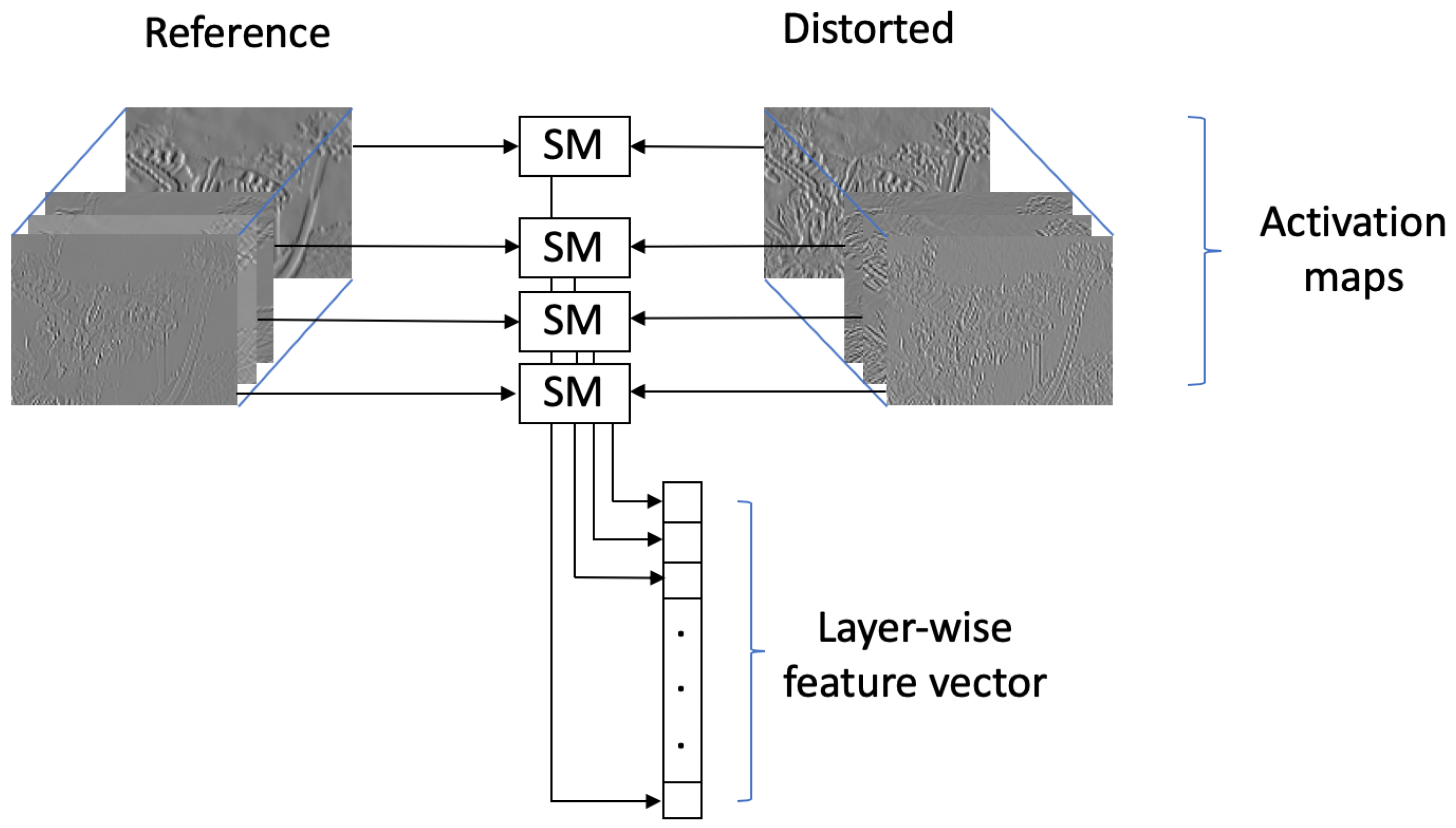
Figure 3.
Areference-distorted image pair fromKADID-10k [44]. (a) Reference image. (b)Distorted image.
Figure 3.
Areference-distorted image pair fromKADID-10k [44]. (a) Reference image. (b)Distorted image.
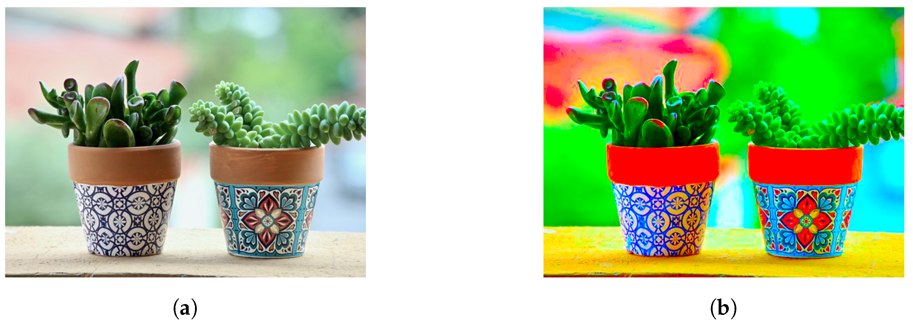
Figure 4.
Activation map visualization of a reference-distorted image pair. (a) Visualization of the first 16 activation maps of AlexNet’s [4] conv1 layer using the reference image in Figure 3a. (b) Visualization of the first 16 activation maps of AlexNet’s [4] conv1 layer using the distorted image in Figure 3b.

Figure 5.
Parameter study with respect to the applied regression techniques and image similarity metrics. (a) Linear SVR. (b) Gaussian SVR. (c) GPR with rational quadratic kernel function.
Figure 5.
Parameter study with respect to the applied regression techniques and image similarity metrics. (a) Linear SVR. (b) Gaussian SVR. (c) GPR with rational quadratic kernel function.

Figure 6.
Plots of mean PLCC, SROCC, and KROCC between ground-truth and predicted MOS values measured on KADID-10k [44] over 100 random train-test splits as a function of the percentage of the dataset used for training. Mean PLCC, SROCC, and KROCC are plotted as red lines, while the standard deviations are depicted as shaded areas. (a) Mean PLCC as a function of the dataset used for training. (b) Mean SROCC as a function of the dataset used for training. (c) Mean KROCC as a function of the dataset used for training.


Figure 7.
Scatter plots of the ground-truth MOS against the predicted MOS of ActMapFeat on different test sets of MDID [48], TID2008 [46], TID2013 [53], VCL-FER [47], KADID-10k [44], and CSIQ [49] IQA benchmark databases. (a) MDID [48]. (b) TID2008 [46]. (c) TID2013 [53]. (d) VCL-FER [47]. (e) KADID-10k [44]. (f) CSIQ [49].

Figure 8.
Box plots of the measured PLCC, SROCC, and KROCC values produced by the proposed ActMapFeat over 100 random train-test splits on MDID [48], TID2008 [46], TID2013 [53], VCL-FER [47], KADID-10k [44], and CSIQ [49] IQA benchmark databases. (a) MDID [48]. (b) TID2008 [46]. (c) TID2013 [53]. (d) VCL-FER [47]. (e) KADID-10k [44]. (f) CSIQ [49].

Figure 9.
Results of the cross database test in matrix form. The proposed ActMapFeat was trained on one given IQA benchmark database (horizontal edge) and tested on another one (vertical edge).
Figure 9.
Results of the cross database test in matrix form. The proposed ActMapFeat was trained on one given IQA benchmark database (horizontal edge) and tested on another one (vertical edge).

Table 1.
Comparison of publicly available image quality analysis (IQA) databases used in this study.
Table 1.
Comparison of publicly available image quality analysis (IQA) databases used in this study.
| Database | Ref. Images | Test Images | Resolution | Distortion Levels | Number of Distortions |
|---|---|---|---|---|---|
| TID2008 [46] | 25 | 1700 | 4 | 17 | |
| CSIQ [49] | 30 | 866 | 4–5 | 6 | |
| VCL-FER [47] | 23 | 552 | 6 | 4 | |
| TID2013 [53] | 25 | 3000 | 5 | 24 | |
| MDID [48] | 20 | 1600 | 4 | 5 | |
| KADID-10k [44] | 81 | 10,125 | 5 | 25 |
Table 2.
Mean PLCC, SROCC, KROCC values of the proposed architecture for each distortion type of KADID-10k [44]. Measured over 100 random train-test splits. The distortion types found in KADID-10k can be classified into five groups: blurs, color distortions, compression, noise, brightness change, spatial distortions, and sharpness and contrast.
| Distortion | PLCC | SROCC | KROCC |
|---|---|---|---|
| Gaussian blur | 0.987 | 0.956 | 0.828 |
| Lens blur | 0.971 | 0.923 | 0.780 |
| Motion blur | 0.976 | 0.960 | 0.827 |
| Color diffusion | 0.971 | 0.906 | 0.744 |
| Color shift | 0.942 | 0.866 | 0.698 |
| Color quantization | 0.902 | 0.868 | 0.692 |
| Color saturation 1. | 0.712 | 0.654 | 0.484 |
| Color saturation 2. | 0.973 | 0.945 | 0.798 |
| JPEG2000 | 0.977 | 0.941 | 0.800 |
| JPEG | 0.983 | 0.897 | 0.741 |
| White noise | 0.921 | 0.919 | 0.758 |
| White noise in color component | 0.958 | 0.946 | 0.802 |
| Impulse noise | 0.875 | 0.872 | 0.694 |
| Multiplicative noise | 0.958 | 0.952 | 0.813 |
| Denoise | 0.955 | 0.941 | 0.799 |
| Brighten | 0.969 | 0.951 | 0.815 |
| Darken | 0.973 | 0.919 | 0.769 |
| Mean shift | 0.778 | 0.777 | 0.586 |
| Jitter | 0.981 | 0.962 | 0.834 |
| Non-eccentricity patch | 0.693 | 0.667 | 0.489 |
| Pixelate | 0.909 | 0.854 | 0.681 |
| Quantization | 0.893 | 0.881 | 0.705 |
| Color block | 0.647 | 0.539 | 0.386 |
| High sharpen | 0.948 | 0.938 | 0.786 |
| Contrast change | 0.802 | 0.805 | 0.607 |
| All | 0.959 | 0.957 | 0.819 |
Table 3.
Mean PLCC, SROCC, KROCC values of the proposed architecture for each distortion level of KADID-10k [44]. Measured over 100 random train-test splits. KADID-10k [44] contains images with five different distortion levels, where Level 1 stands for the lowest amount of distortion, while Level 5 denotes the highest amount.
| Level of Distortion | PLCC | SROCC | KROCC |
|---|---|---|---|
| Level 1 | 0.889 | 0.843 | 0.659 |
| Level 2 | 0.924 | 0.918 | 0.748 |
| Level 3 | 0.935 | 0.933 | 0.777 |
| Level 4 | 0.937 | 0.922 | 0.765 |
| Level 5 | 0.931 | 0.897 | 0.725 |
| All | 0.959 | 0.957 | 0.819 |
Table 4.
Performance comparison on KADID-10k [44] and TID2013 [53] databases. Mean PLCC, SROCC, and KROCC values are reported for the learning-based approaches measured over 100 random train-test splits. The best results are typed in bold. The green background color stands for the fact that the correlation is lower than those of the proposed method and the difference is statistically significant with p < 0.05. We used ‘-’ if the data were not available.
| KADID-10k [44] | TID2013 [53] | |||||
|---|---|---|---|---|---|---|
| PLCC | SROCC | KROCC | PLCC | SROCC | KROCC | |
| SSIM [12] | 0.670 | 0.671 | 0.489 | 0.618 | 0.616 | 0.437 |
| MS-SSIM [14] | 0.819 | 0.821 | 0.630 | 0.794 | 0.785 | 0.604 |
| MAD [49] | 0.716 | 0.724 | 0.535 | 0.827 | 0.778 | 0.600 |
| GSM [56] | 0.780 | 0.780 | 0.588 | 0.789 | 0.787 | 0.593 |
| HaarPSI [20] | 0.871 | 0.885 | 0.699 | 0.886 | 0.859 | 0.678 |
| MDSI [57] | 0.887 | 0.885 | 0.702 | 0.867 | 0.859 | 0.677 |
| CSV [58] | 0.671 | 0.669 | 0.531 | 0.852 | 0.848 | 0.657 |
| GMSD [19] | 0.847 | 0.847 | 0.664 | 0.846 | 0.844 | 0.663 |
| DSS [59] | 0.855 | 0.860 | 0.674 | 0.793 | 0.781 | 0.604 |
| VSI [60] | 0.874 | 0.861 | 0.678 | 0.900 | 0.894 | 0.677 |
| PerSIM [61] | 0.819 | 0.824 | 0.634 | 0.825 | 0.826 | 0.655 |
| BLeSS-SR-SIM [62] | 0.820 | 0.824 | 0.633 | 0.814 | 0.828 | 0.648 |
| BLeSS-FSIM [62] | 0.814 | 0.816 | 0.624 | 0.824 | 0.830 | 0.649 |
| BLeSS-FSIMc [62] | 0.845 | 0.848 | 0.658 | 0.846 | 0.849 | 0.667 |
| LCSIM1 [40] | - | - | - | 0.914 | 0.904 | 0.733 |
| ReSIFT [63] | 0.648 | 0.628 | 0.468 | 0.630 | 0.623 | 0.471 |
| IQ() [28] | 0.853 | 0.852 | 0.641 | 0.844 | 0.842 | 0.631 |
| MS-UNIQUE [64] | 0.845 | 0.840 | 0.648 | 0.865 | 0.871 | 0.687 |
| SSIM CNN [41] | 0.811 | 0.814 | 0.630 | 0.759 | 0.752 | 0.566 |
| RVSIM [65] | 0.728 | 0.719 | 0.540 | 0.763 | 0.683 | 0.520 |
| 2stepQA [66] | 0.768 | 0.771 | 0.571 | 0.736 | 0.733 | 0.550 |
| SUMMER [67] | 0.719 | 0.723 | 0.540 | 0.623 | 0.622 | 0.472 |
| CEQI [68] | 0.862 | 0.863 | 0.681 | 0.855 | 0.802 | 0.635 |
| CEQIc [68] | 0.867 | 0.864 | 0.682 | 0.858 | 0.851 | 0.638 |
| VCGS [69] | 0.873 | 0.871 | 0.683 | 0.900 | 0.893 | 0.712 |
| DISTS [70] | 0.809 | 0.814 | 0.626 | 0.759 | 0.711 | 0.524 |
| DeepFL-IQA [42] | 0.938 | 0.936 | - | 0.876 | 0.858 | - |
| BLINDER [43] | - | - | - | 0.819 | 0.838 | - |
| RankIQA [71] | - | - | - | 0.799 | 0.780 | - |
| BPSOM-MD [72] | - | - | - | 0.879 | 0.863 | - |
| NSSADNN [73] | - | - | - | 0.910 | 0.844 | - |
| ActMapFeat (ours) | 0.959 | 0.957 | 0.819 | 0.943 | 0.936 | 0.780 |
Table 5.
Performance comparison on VCL-FER [47] and TID2008 [46] databases. Mean PLCC, SROCC, and KROCC values are reported for the learning-based approaches measured over 100 random train-test splits. The best results are typed in bold. The green background color stands for the fact that the correlation is lower than those of the proposed method and the difference is statistically significant with p < 0.05. We used ‘-’ if the data were not available.
| VCL-FER [47] | TID2008 [46] | |||||
|---|---|---|---|---|---|---|
| PLCC | SROCC | KROCC | PLCC | SROCC | KROCC | |
| SSIM [12] | 0.751 | 0.859 | 0.666 | 0.669 | 0.675 | 0.485 |
| MS-SSIM [14] | 0.917 | 0.925 | 0.753 | 0.838 | 0.846 | 0.648 |
| MAD [49] | 0.904 | 0.906 | 0.721 | 0.831 | 0.829 | 0.639 |
| GSM [56] | 0.904 | 0.905 | 0.721 | 0.782 | 0.781 | 0.578 |
| HaarPSI [20] | 0.938 | 0.946 | 0.789 | 0.916 | 0.897 | 0.723 |
| MDSI [57] | 0.935 | 0.939 | 0.774 | 0.877 | 0.892 | 0.724 |
| CSV [58] | 0.951 | 0.952 | 0.798 | 0.852 | 0.851 | 0.659 |
| GMSD [19] | 0.918 | 0.918 | 0.741 | 0.879 | 0.879 | 0.696 |
| DSS [59] | 0.925 | 0.927 | 0.757 | 0.860 | 0.860 | 0.672 |
| VSI [60] | 0.929 | 0.932 | 0.763 | 0.898 | 0.896 | 0.709 |
| PerSIM [61] | 0.926 | 0.928 | 0.761 | 0.826 | 0.830 | 0.655 |
| BLeSS-SR-SIM [62] | 0.899 | 0.909 | 0.727 | 0.846 | 0.850 | 0.672 |
| BLeSS-FSIM [62] | 0.927 | 0.924 | 0.751 | 0.853 | 0.851 | 0.669 |
| BLeSS-FSIMc [62] | 0.932 | 0.935 | 0.768 | 0.871 | 0.871 | 0.687 |
| LCSIM1 [40] | - | - | - | 0.896 | 0.906 | 0.727 |
| ReSIFT [63] | 0.914 | 0.917 | 0.733 | 0.627 | 0.632 | 0.484 |
| IQ() [28] | 0.910 | 0.912 | 0.718 | 0.841 | 0.840 | 0.629 |
| MS-UNIQUE [64] | 0.954 | 0.956 | 0.840 | 0.846 | 0.869 | 0.681 |
| SSIM CNN [41] | 0.917 | 0.921 | 0.743 | 0.770 | 0.737 | 0.551 |
| RVSIM [65] | 0.894 | 0.901 | 0.719 | 0.789 | 0.743 | 0.566 |
| 2stepQA [66] | 0.883 | 0.887 | 0.698 | 0.757 | 0.769 | 0.574 |
| SUMMER [67] | 0.750 | 0.754 | 0.596 | 0.817 | 0.823 | 0.637 |
| CEQI [68] | 0.894 | 0.920 | 0.747 | 0.887 | 0.891 | 0.714 |
| CEQIc [68] | 0.906 | 0.918 | 0.744 | 0.892 | 0.895 | 0.719 |
| VCGS [69] | 0.940 | 0.937 | 0.773 | 0.878 | 0.887 | 0.705 |
| DISTS [70] | 0.923 | 0.922 | 0.746 | 0.705 | 0.668 | 0.488 |
| DeepFL-IQA [42] | - | - | - | - | - | - |
| BLINDER [43] | - | - | - | - | - | - |
| RankIQA [71] | - | - | - | - | - | - |
| BPSOM-MD [72] | - | - | - | - | - | - |
| NSSADNN [73] | - | - | - | - | - | - |
| ActMapFeat (ours) | 0.960 | 0.961 | 0.826 | 0.941 | 0.937 | 0.790 |
Table 6.
Performance comparison on MDID [48] and CSIQ [49] databases. Mean PLCC, SROCC, and KROCC values are reported for the learning-based approaches measured over 100 random train-test splits. The best results are typed in bold. The green background color stands for the fact that the correlation is lower than those of the proposed method and the difference is statistically significant with p < 0.05. We used ‘-’ if the data were not available.
| MDID [48] | CSIQ [49] | |||||
|---|---|---|---|---|---|---|
| PLCC | SROCC | KROCC | PLCC | SROCC | KROCC | |
| SSIM [12] | 0.581 | 0.576 | 0.411 | 0.812 | 0.812 | 0.606 |
| MS-SSIM [14] | 0.836 | 0.841 | 0.654 | 0.913 | 0.917 | 0.743 |
| MAD [49] | 0.742 | 0.725 | 0.533 | 0.950 | 0.947 | 0.796 |
| GSM [56] | 0.825 | 0.827 | 0.636 | 0.906 | 0.910 | 0.729 |
| HaarPSI [20] | 0.904 | 0.903 | 0.734 | 0.946 | 0.960 | 0.823 |
| MDSI [57] | 0.829 | 0.836 | 0.653 | 0.953 | 0.957 | 0.812 |
| CSV [58] | 0.879 | 0.881 | 0.700 | 0.933 | 0.933 | 0.766 |
| GMSD [19] | 0.864 | 0.862 | 0.680 | 0.954 | 0.957 | 0.812 |
| DSS [59] | 0.870 | 0.866 | 0.679 | 0.953 | 0.955 | 0.811 |
| VSI [60] | 0.855 | 0.857 | 0.671 | 0.928 | 0.942 | 0.785 |
| PerSIM [61] | 0.823 | 0.820 | 0.630 | 0.924 | 0.929 | 0.768 |
| BLeSS-SR-SIM [62] | 0.805 | 0.815 | 0.626 | 0.892 | 0.893 | 0.718 |
| BLeSS-FSIM [62] | 0.848 | 0.847 | 0.658 | 0.882 | 0.885 | 0.701 |
| BLeSS-FSIMc [62] | 0.878 | 0.883 | 0.702 | 0.913 | 0.917 | 0.743 |
| LCSIM1 [40] | - | - | - | 0.897 | 0.949 | 0.799 |
| ReSIFT [63] | 0.905 | 0.895 | 0.716 | 0.884 | 0.868 | 0.695 |
| IQ() [28] | 0.867 | 0.865 | 0.708 | 0.915 | 0.912 | 0.720 |
| MS-UNIQUE [64] | 0.863 | 0.871 | 0.689 | 0.918 | 0.929 | 0.759 |
| SSIM CNN [41] | 0.904 | 0.907 | 0.732 | 0.952 | 0.946 | 0.794 |
| RVSIM [65] | 0.884 | 0.884 | 0.709 | 0.923 | 0.903 | 0.728 |
| 2stepQA [66] | 0.753 | 0.759 | 0.562 | 0.841 | 0.849 | 0.655 |
| SUMMER [67] | 0.742 | 0.734 | 0.543 | 0.826 | 0.830 | 0.658 |
| CEQI [68] | 0.863 | 0.864 | 0.685 | 0.956 | 0.956 | 0.814 |
| CEQIc [68] | 0.864 | 0.863 | 0.684 | 0.956 | 0.955 | 0.810 |
| VCGS [69] | 0.867 | 0.869 | 0.687 | 0.931 | 0.944 | 0.790 |
| DISTS [70] | 0.862 | 0.860 | 0.669 | 0.930 | 0.930 | 0.764 |
| DeepFL-IQA [42] | - | - | - | 0.946 | 0.930 | - |
| BLINDER [43] | - | - | - | 0.968 | 0.961 | - |
| RankIQA [71] | - | - | - | 0.960 | 0.947 | - |
| BPSOM-MD [72] | - | - | - | 0.860 | 0.904 | - |
| NSSADNN [73] | - | - | - | 0.927 | 0.893 | - |
| ActMapFeat(ours) | 0.930 | 0.927 | 0.769 | 0.971 | 0.970 | 0.850 |
Publisher’s Note: MDPI stays neutral with regard to jurisdictional claims in published maps and institutional affiliations. |
© 2020 by the author. Licensee MDPI, Basel, Switzerland. This article is an open access article distributed under the terms and conditions of the Creative Commons Attribution (CC BY) license (http://creativecommons.org/licenses/by/4.0/).
Share and Cite
MDPI and ACS Style
Varga, D. A Combined Full-Reference Image Quality Assessment Method Based on Convolutional Activation Maps. Algorithms 2020, 13, 313. https://doi.org/10.3390/a13120313
AMA Style
Varga D. A Combined Full-Reference Image Quality Assessment Method Based on Convolutional Activation Maps. Algorithms. 2020; 13(12):313. https://doi.org/10.3390/a13120313
Chicago/Turabian StyleVarga, Domonkos. 2020. "A Combined Full-Reference Image Quality Assessment Method Based on Convolutional Activation Maps" Algorithms 13, no. 12: 313. https://doi.org/10.3390/a13120313
Note that from the first issue of 2016, this journal uses article numbers instead of page numbers. See further details here.