Re-Pair in Small Space †

 ,
,  , , ,
, , ,
Abstract
1. Introduction
1.1. Related Work
1.2. Our Contribution
1.3. Preliminaries
2. Sequential Algorithm
2.1. Trade-Off Computation
2.2. Algorithmic Ideas
| Algorithm 1: Algorithmic outline of our proposed algorithm working on a text T with a growing frequency table F. The constants and are explained in Section 2.3. The same section shows that the outer while loop is executed times. |
 |
2.3. Algorithmic Details
- 1.
- the frequencies of ab and cd decrease by one (for the border case a = b = c (resp. b = c = d), there is no need to decrement the frequency of ab (resp. cd)), and
- 2.
- the frequencies of and increase by one.
- 1.
- The first item in this maximum function allows us to spend bits for each freed character such that we obtain space for one additional entry in F after freeing characters.
- 2.
- The second item allows us to use additional bits after freeing up c characters. This additional treatment helps us to let grow sufficiently fast in the first steps to save our time bound, as for sufficiently small alphabets and large text sizes, , which means that we might run the first turns with and, therefore, already spend time. Hence, after freeing up characters, we have space to store one additional entry in F.
2.4. Storing the Output In-Place
- (a)
- append to A,
- (b)
- replace and with a new non-terminal to transform to , and
- (c)
- recurse on with until no bigram with frequency two is left.
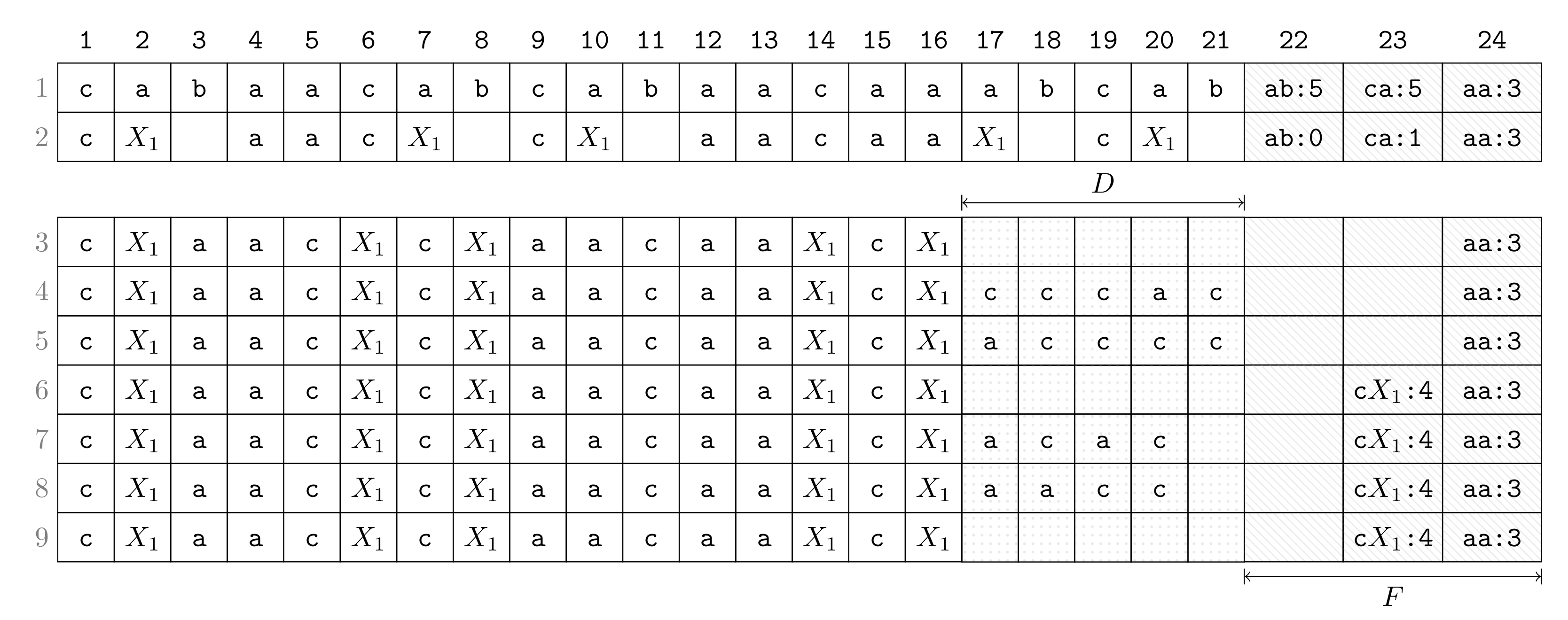
2.5. Step-by-Step Execution
- Row 1:
- Suppose that we have computed F, which has the constant number of entries (in the later turns when the size becomes larger, F will be put in the text space). The highest frequency is five achieved by and . The lowest frequency represented in F is three, which becomes the threshold for a bigram to be present in F such that bigrams whose frequencies drop below are removed from F. This threshold is a constant for all later turns until F is rebuilt (in the following round). During Turn 1, the algorithm proceeds now as follows:
- Row 2:
- Choose as a bigram to replace with a new non-terminal (break ties arbitrarily). Replace every occurrence of with while decrementing frequencies in F according to the neighboring characters of the replaced occurrence.
- Row 3:
- Remove from F every bigram whose frequency falls below the threshold. Obtain space for D by aligning the compressed text (the process of Row 2 and Row 3 can be done simultaneously).
- Row 4:
- Scan the text and copy each character preceding an occurrence of in to D.
- Row 5:
- Sort characters in D lexicographically.
- Row 6:
- Insert new bigrams (consisting of a character of D and ) whose frequencies are at least as large as the threshold.
- Row 7:
- Scan the text again and copy each character succeeding an occurrence of in to D (symmetric to Row 4).
- Row 8:
- Sort all characters in D lexicographically (symmetric to Row 5).
- Row 9:
- Insert new bigrams whose frequencies are at least as large as the threshold (symmetric to Row 6).
2.6. Implementation
3. Bit-Parallel Algorithm
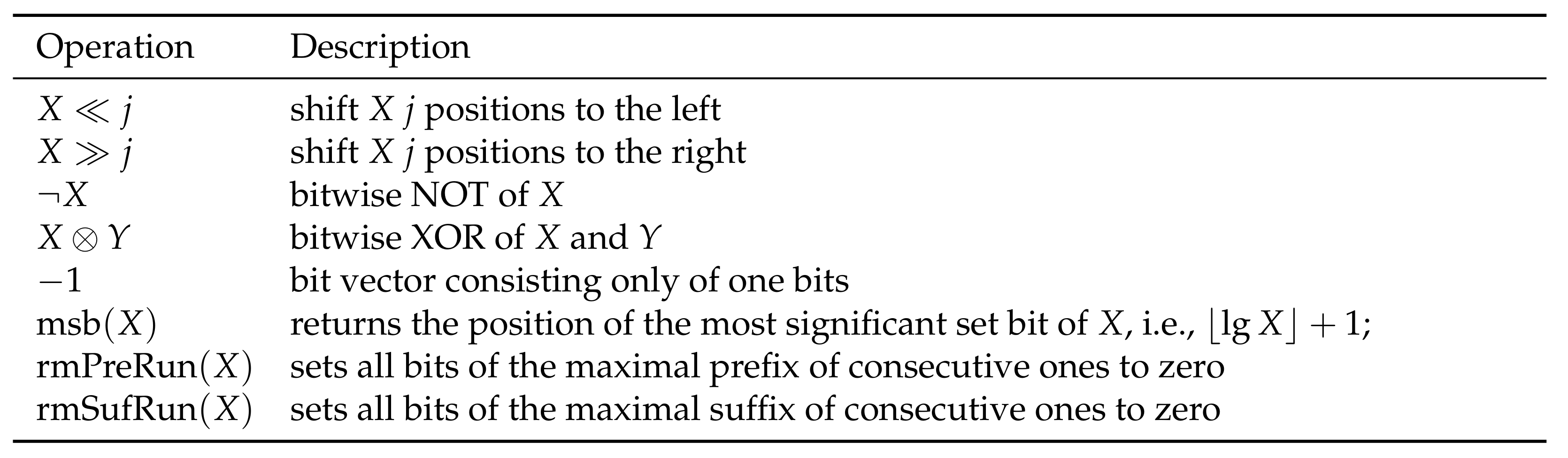
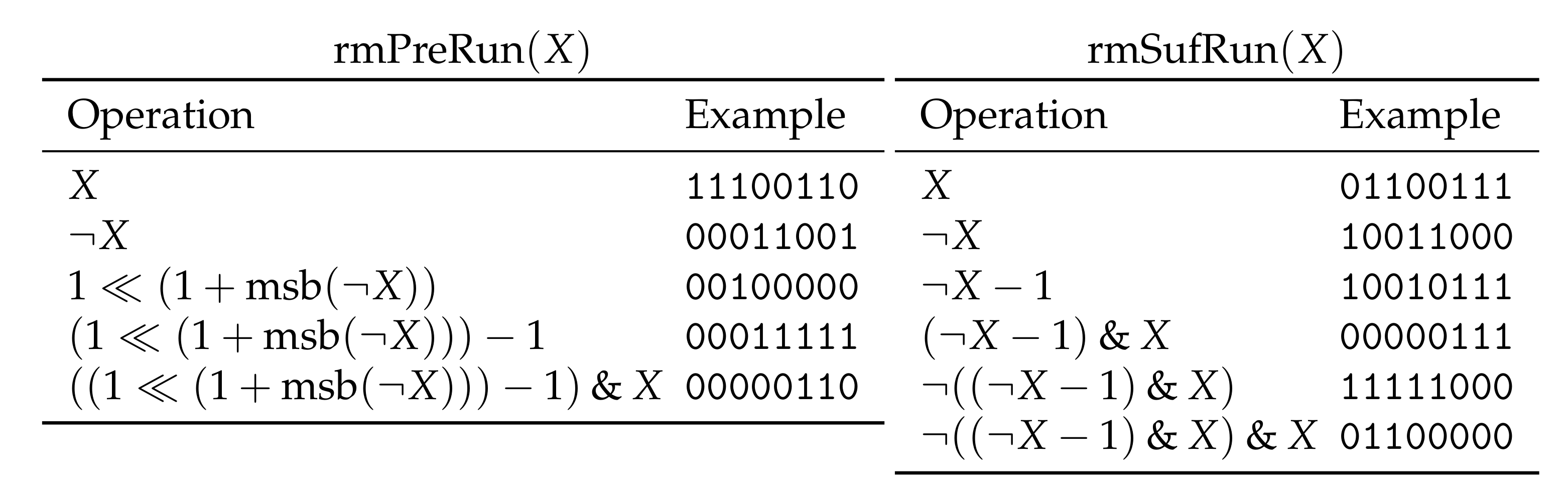
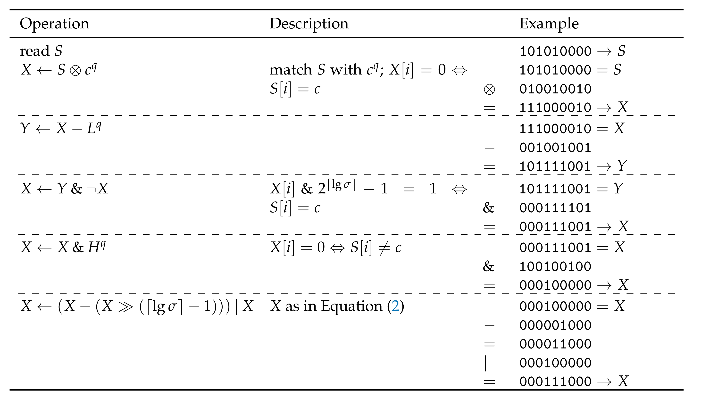
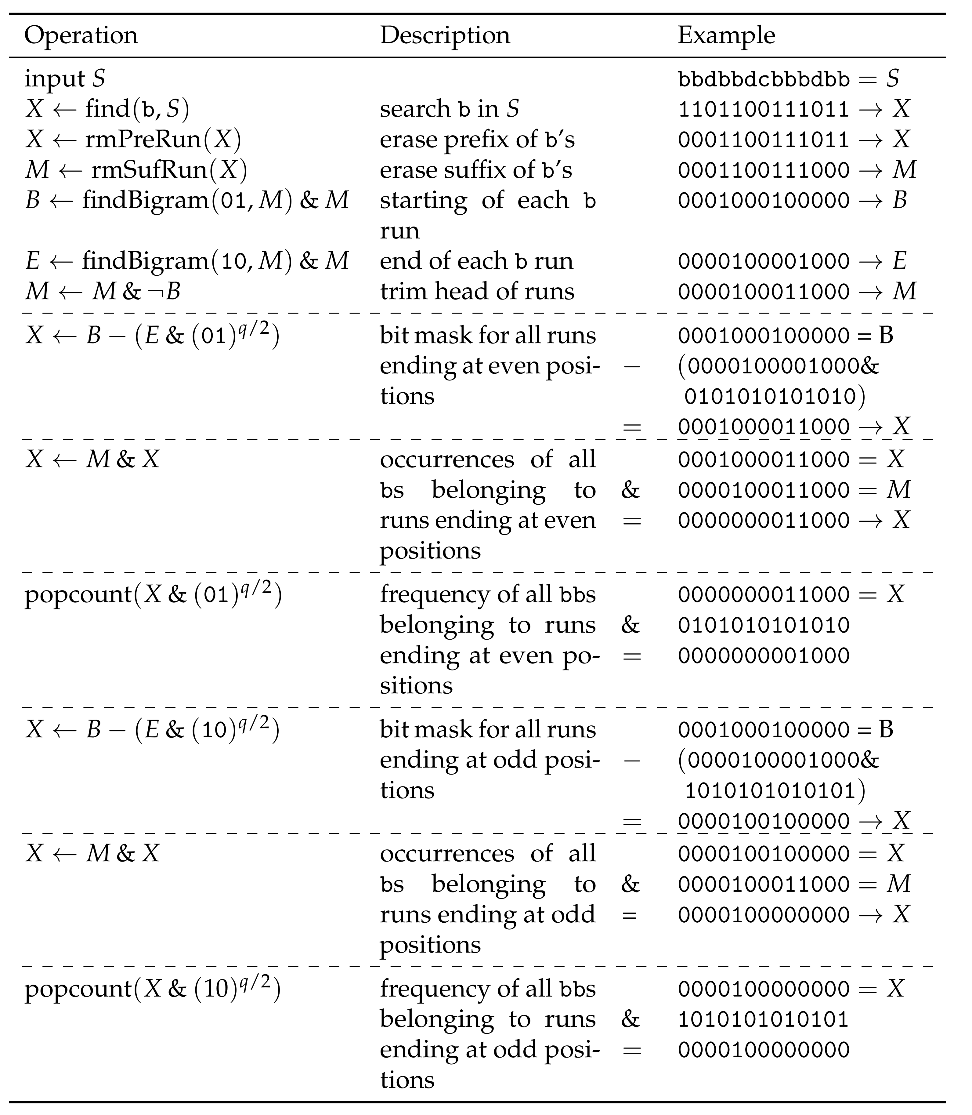
3.1. Broadword Search
3.2. Bit-Parallel Adaption
- (1)
- replacing all occurrences of a bigram,
- (2)
- shifting freed up text space to the right,
- (3)
- finding the bigram with the highest or lowest frequency in F,
- (4)
- updating or exchanging an entry in F, and
- (5)
- looking up the frequency of a bigram in F.
4. Computing MR-Re-Pair in Small Space
5. Parallel Algorithm
| Operation | Lemma 2 | Parallel |
| fill with bigrams | ||
| sort lexicographically | ||
| compute frequencies of | ||
| merge with F |
| Operation | Sequential | Parallel |
| linearly scan F | ||
| linearly scan | ||
| sort D with |
6. Computing Re-Pair in External Memory
7. Heuristics for Practicality
- 1.
- bits,
- 2.
- bits, or
- 3.
- bits.
8. Conclusions
Author Contributions
Funding
Institutional Review Board Statement
Informed Consent Statement
Data Availability Statement
Conflicts of Interest
References
- Larsson, N.J.; Moffat, A. Offline Dictionary-Based Compression. In Proceedings of the 1999 Data Compression Conference, Snowbird, UT, USA, 29–31 March 1999; pp. 296–305. [Google Scholar]
- Navarro, G.; Russo, L.M.S. Re-Pair Achieves High-Order Entropy. In Proceedings of the 2008 Data Compression Conference, Snowbird, UT, USA, 25–27 March 2008; p. 537. [Google Scholar]
- Kieffer, J.C.; Yang, E. Grammar-based codes: A new class of universal lossless source codes. IEEE Trans. Inf. Theory 2000, 46, 737–754. [Google Scholar] [CrossRef]
- Ochoa, C.; Navarro, G. RePair and All Irreducible Grammars are Upper Bounded by High-Order Empirical Entropy. IEEE Trans. Inf. Theory 2019, 65, 3160–3164. [Google Scholar] [CrossRef]
- Ganczorz, M. Entropy Lower Bounds for Dictionary Compression. Proc. CPM 2019, 128, 11:1–11:18. [Google Scholar]
- Charikar, M.; Lehman, E.; Liu, D.; Panigrahy, R.; Prabhakaran, M.; Sahai, A.; Shelat, A. The smallest grammar problem. IEEE Trans. Inf. Theory 2005, 51, 2554–2576. [Google Scholar] [CrossRef]
- Bannai, H.; Hirayama, M.; Hucke, D.; Inenaga, S.; Jez, A.; Lohrey, M.; Reh, C.P. The smallest grammar problem revisited. arXiv 2019, arXiv:1908.06428. [Google Scholar] [CrossRef]
- Yoshida, S.; Kida, T. Effective Variable-Length-to-Fixed-Length Coding via a Re-Pair Algorithm. In Proceedings of the 2013 Data Compression Conference, Snowbird, UT, USA, 20–22 March 2013; p. 532. [Google Scholar]
- Lohrey, M.; Maneth, S.; Mennicke, R. XML tree structure compression using RePair. Inf. Syst. 2013, 38, 1150–1167. [Google Scholar] [CrossRef]
- Tabei, Y.; Saigo, H.; Yamanishi, Y.; Puglisi, S.J. Scalable Partial Least Squares Regression on Grammar-Compressed Data Matrices. In Proceedings of the SIGKDD, San Francisco, CA, USA, 13–17 August 2016; pp. 1875–1884. [Google Scholar]
- de Luca, P.; Russiello, V.M.; Ciro-Sannino, R.; Valente, L. A study for Image compression using Re-Pair algorithm. arXiv 2019, arXiv:1901.10744. [Google Scholar]
- Claude, F.; Navarro, G. Fast and Compact Web Graph Representations. TWEB 2010, 4, 16:1–16:31. [Google Scholar] [CrossRef]
- González, R.; Navarro, G.; Ferrada, H. Locally Compressed Suffix Arrays. ACM J. Exp. Algorithmics 2014, 19, 1. [Google Scholar] [CrossRef]
- Sekine, K.; Sasakawa, H.; Yoshida, S.; Kida, T. Adaptive Dictionary Sharing Method for Re-Pair Algorithm. In Proceedings of the 2014 Data Compression Conference, Snowbird, UT, USA, 26–28 March 2014; p. 425. [Google Scholar]
- Masaki, T.; Kida, T. Online Grammar Transformation Based on Re-Pair Algorithm. In Proceedings of the 2016 Data Compression Conference (DCC), Snowbird, UT, USA, 30 March–1 April 2016; pp. 349–358. [Google Scholar]
- Ganczorz, M.; Jez, A. Improvements on Re-Pair Grammar Compressor. In Proceedings of the 2017 Data Compression Conference (DCC), Snowbird, UT, USA, 4–7 April 2017; pp. 181–190. [Google Scholar]
- Ziv, J.; Lempel, A. A universal algorithm for sequential data compression. IEEE Trans. Inf. Theory 1977, 23, 337–343. [Google Scholar] [CrossRef]
- Furuya, I.; Takagi, T.; Nakashima, Y.; Inenaga, S.; Bannai, H.; Kida, T. MR-RePair: Grammar Compression based on Maximal Repeats. In Proceedings of the 2019 Data Compression Conference (DCC), Snowbird, UT, USA, 26–29 March 2019; pp. 508–517. [Google Scholar]
- Kärkkäinen, J.; Kempa, D.; Puglisi, S.J. Lightweight Lempel-Ziv Parsing. In Proceedings of the International Symposium on Experimental Algorithms, Rome, Italy, 5–7 June 2013; Volume 7933, pp. 139–150. [Google Scholar]
- Goto, K. Optimal Time and Space Construction of Suffix Arrays and LCP Arrays for Integer Alphabets. In Proceedings of the Prague Stringology Conference 2019, Prague, Czech Republic, 26–28 August 2019; pp. 111–125. [Google Scholar]
- Manber, U.; Myers, E.W. Suffix Arrays: A New Method for On-Line String Searches. SIAM J. Comput. 1993, 22, 935–948. [Google Scholar] [CrossRef]
- Li, Z.; Li, J.; Huo, H. Optimal In-Place Suffix Sorting. In Proceedings of the International Symposium on String Processing and Information Retrieval, Lima, Peru, 9–11 October 2018; Volume 11147, pp. 268–284. [Google Scholar]
- Crochemore, M.; Grossi, R.; Kärkkäinen, J.; Landau, G.M. Computing the Burrows-Wheeler transform in place and in small space. J. Discret. Algorithms 2015, 32, 44–52. [Google Scholar] [CrossRef]
- da Louza, F.A.; Gagie, T.; Telles, G.P. Burrows-Wheeler transform and LCP array construction in constant space. J. Discret. Algorithms 2017, 42, 14–22. [Google Scholar] [CrossRef]
- Kosolobov, D. Faster Lightweight Lempel-Ziv Parsing. In Proceedings of the International Symposium on Mathematical Foundations of Computer Science, Milano, Italy, 24–28 August 2015; Volume 9235, pp. 432–444. [Google Scholar]
- Nakamura, R.; Inenaga, S.; Bannai, H.; Funamoto, T.; Takeda, M.; Shinohara, A. Linear-Time Text Compression by Longest-First Substitution. Algorithms 2009, 2, 1429–1448. [Google Scholar] [CrossRef]
- Bille, P.; Gørtz, I.L.; Prezza, N. Space-Efficient Re-Pair Compression. In Proceedings of the 2017 Data Compression Conference (DCC), Snowbird, UT, USA, 4–7 April 2017; pp. 171–180. [Google Scholar]
- Bille, P.; Gørtz, I.L.; Prezza, N. Practical and Effective Re-Pair Compression. arXiv 2017, arXiv:1704.08558. [Google Scholar]
- Sakai, K.; Ohno, T.; Goto, K.; Takabatake, Y.; I, T.; Sakamoto, H. RePair in Compressed Space and Time. In Proceedings of the 2019 Data Compression Conference (DCC), Snowbird, UT, USA, 26–29 March 2019; pp. 518–527. [Google Scholar]
- Carrascosa, R.; Coste, F.; Gallé, M.; López, G.G.I. Choosing Word Occurrences for the Smallest Grammar Problem. In Proceedings of the International Conference on Language and Automata Theory and Applications, Trier, Germany, 24–28 May 2010; Volume 6031, pp. 154–165. [Google Scholar]
- Gage, P. A New Algorithm for Data Compression. C Users J. 1994, 12, 23–38. [Google Scholar]
- Chan, T.M.; Munro, J.I.; Raman, V. Selection and Sorting in the “Restore” Model. ACM Trans. Algorithms 2018, 14, 11:1–11:18. [Google Scholar] [CrossRef]
- Williams, J.W.J. Algorithm 232—Heapsort. Commun. ACM 1964, 7, 347–348. [Google Scholar]
- Vigna, S. Broadword Implementation of Rank/Select Queries. In Proceedings of the International Workshop on Experimental and Efficient Algorithms, Provincetown, MA, USA, 30 May–1 June 2008; Volume 5038, pp. 154–168. [Google Scholar]
- Fredman, M.L.; Willard, D.E. Surpassing the Information Theoretic Bound with Fusion Trees. J. Comput. Syst. Sci. 1993, 47, 424–436. [Google Scholar] [CrossRef]
- Knuth, D.E. The Art of Computer Programming, Volume 4, Fascicle 1: Bitwise Tricks & Techniques; Binary Decision Diagrams, 12th ed.; Addison-Wesley: Boston, MA, USA, 2009. [Google Scholar]
- Batcher, K.E. Sorting Networks and Their Applications. In Proceedings of the AFIPS Spring Joint Computer Conference, Atlantic City, NJ, USA, 30 April–2 May 1968; Volume 32, pp. 307–314. [Google Scholar]
- Aggarwal, A.; Vitter, J.S. The Input/Output Complexity of Sorting and Related Problems. Commun. ACM 1988, 31, 1116–1127. [Google Scholar] [CrossRef]
- Jiang, S.; Larsen, K.G. A Faster External Memory Priority Queue with DecreaseKeys. In Proceedings of the 2019 Annual ACM-SIAM Symposium on Discrete Algorithms, San Diego, CA, USA, 6–9 January 2019; pp. 1331–1343. [Google Scholar]
- Simic, S. Jensen’s inequality and new entropy bounds. Appl. Math. Lett. 2009, 22, 1262–1265. [Google Scholar] [CrossRef]
- Boyer, R.S.; Moore, J.S. MJRTY: A Fast Majority Vote Algorithm. In Automated Reasoning: Essays in Honor of Woody Bledsoe; Automated Reasoning Series; Springer: Dordrecht, The Netherlands, 1991; pp. 105–118. [Google Scholar]
- Köppl, D.; Furuya, I.; Takabatake, Y.; Sakai, K.; Goto, K. Re-Pair in Small Space. In Proceedings of the Prague Stringology Conference 2020, Prague, Czech Republic, 31 August–2 September 2020; pp. 134–147. [Google Scholar]
- Köppl, D.; I, T.; Furuya, I.; Takabatake, Y.; Sakai, K.; Goto, K. Re-Pair in Small Space (Poster). In Proceedings of the 2020 Data Compression Conference, Snowbird, UT, USA, 24–27 March 2020; p. 377. [Google Scholar]


| Data Set | Our Implementation | Implementation of Navarro | ||||||||
|---|---|---|---|---|---|---|---|---|---|---|
| Prefix Size in KiB | ||||||||||
| 64 | 128 | 256 | 512 | 1024 | 64 | 128 | 256 | 512 | 1024 | |
| Escherichia_Coli | 20.68 | 130.47 | 516.67 | 1708.02 | 10,112.47 | 0.01 | 0.02 | 0.07 | 0.18 | 0.29 |
| cere | 13.69 | 90.83 | 443.17 | 2125.17 | 9185.58 | 0.01 | 0.02 | 0.04 | 0.16 | 0.22 |
| coreutils | 12.88 | 75.64 | 325.51 | 1502.89 | 5144.18 | 0.01 | 0.05 | 0.05 | 0.14 | 0.29 |
| einstein.de.txt | 19.55 | 88.34 | 181.84 | 805.81 | 4559.79 | 0.01 | 0.04 | 0.08 | 0.10 | 0.25 |
| einstein.en.txt | 21.11 | 78.57 | 160.41 | 900.79 | 4353.81 | 0.01 | 0.02 | 0.05 | 0.21 | 0.51 |
| influenza | 41.01 | 160.68 | 667.58 | 2630.65 | 10,526.23 | 0.03 | 0.02 | 0.05 | 0.11 | 0.36 |
| kernel | 20.53 | 101.84 | 208.08 | 1575.48 | 5067.80 | 0.01 | 0.04 | 0.09 | 0.18 | 0.27 |
| para | 20.90 | 175.93 | 370.72 | 2826.76 | 9462.74 | 0.01 | 0.01 | 0.08 | 0.12 | 0.35 |
| world_leaders | 11.92 | 21.82 | 167.52 | 661.52 | 1718.36 | 0.01 | 0.01 | 0.06 | 0.11 | 0.25 |
| 0.35 | 0.92 | 3.90 | 14.16 | 61.74 | 0.01 | 0.01 | 0.05 | 0.05 | 0.12 | |
| Data Set | Prefix Size in KiB | ||||
|---|---|---|---|---|---|
| 64 | 128 | 256 | 512 | 1024 | |
| Escherichia_Coli | 0.01 | 0.02 | 0.07 | 0.18 | 0.29 |
| cere | 0.01 | 0.02 | 0.04 | 0.16 | 0.22 |
| coreutils | 0.01 | 0.05 | 0.05 | 0.14 | 0.29 |
| einstein.de.txt | 0.01 | 0.04 | 0.08 | 0.10 | 0.25 |
| einstein.en.txt | 0.01 | 0.02 | 0.05 | 0.21 | 0.51 |
| influenza | 0.03 | 0.02 | 0.05 | 0.11 | 0.36 |
| kernel | 0.01 | 0.04 | 0.09 | 0.18 | 0.27 |
| para | 0.01 | 0.01 | 0.08 | 0.12 | 0.35 |
| world_leaders | 0.01 | 0.01 | 0.06 | 0.11 | 0.25 |
| Data Set | Turns/1000 | Rounds | |||||||||
|---|---|---|---|---|---|---|---|---|---|---|---|
| Prefix Size in KiB | Prefix Size in KiB | ||||||||||
| Escherichia_Coli | 4 | 1.8 | 3.2 | 5.6 | 10.3 | 18.1 | 6 | 9 | 9 | 12 | 12 |
| cere | 5 | 1.4 | 2.8 | 5.0 | 9.2 | 15.1 | 13 | 14 | 14 | 14 | 14 |
| coreutils | 113 | 4.7 | 6.7 | 10.2 | 16.1 | 26.5 | 15 | 15 | 15 | 14 | 14 |
| einstein.de.txt | 95 | 1.7 | 2.8 | 3.7 | 5.2 | 9.7 | 14 | 14 | 15 | 16 | 16 |
| einstein.en.txt | 87 | 3.3 | 3.5 | 3.8 | 4.5 | 8.6 | 16 | 15 | 15 | 15 | 17 |
| influenza | 7 | 2.5 | 3.7 | 9.5 | 13.4 | 22.1 | 11 | 12 | 14 | 13 | 15 |
| kernel | 160 | 4.5 | 8.0 | 13.9 | 24.5 | 43.7 | 10 | 11 | 14 | 14 | 13 |
| para | 5 | 1.8 | 3.2 | 5.8 | 10.1 | 17.6 | 12 | 12 | 13 | 13 | 14 |
| world_leaders | 87 | 2.6 | 4.3 | 6.1 | 10.0 | 42.1 | 11 | 11 | 11 | 11 | 14 |
| 1 | 15 | 16 | 17 | 18 | 19 | 16 | 17 | 18 | 19 | 20 | |
Publisher’s Note: MDPI stays neutral with regard to jurisdictional claims in published maps and institutional affiliations. |
© 2020 by the authors. Licensee MDPI, Basel, Switzerland. This article is an open access article distributed under the terms and conditions of the Creative Commons Attribution (CC BY) license (http://creativecommons.org/licenses/by/4.0/).
Share and Cite
Köppl, D.; I, T.; Furuya, I.; Takabatake, Y.; Sakai, K.; Goto, K. Re-Pair in Small Space. Algorithms 2021, 14, 5. https://doi.org/10.3390/a14010005
Köppl D, I T, Furuya I, Takabatake Y, Sakai K, Goto K. Re-Pair in Small Space. Algorithms. 2021; 14(1):5. https://doi.org/10.3390/a14010005
Chicago/Turabian StyleKöppl, Dominik, Tomohiro I, Isamu Furuya, Yoshimasa Takabatake, Kensuke Sakai, and Keisuke Goto. 2021. "Re-Pair in Small Space" Algorithms 14, no. 1: 5. https://doi.org/10.3390/a14010005
APA StyleKöppl, D., I, T., Furuya, I., Takabatake, Y., Sakai, K., & Goto, K. (2021). Re-Pair in Small Space. Algorithms, 14(1), 5. https://doi.org/10.3390/a14010005