Abstract
In an effort to quantify and manage uncertainties inside power systems with penetration of renewable energy, uncertainty costs have been defined and different uncertainty cost functions have been calculated for different types of generators and electric vehicles. This article seeks to use the uncertainty cost formulation to propose algorithms and solve the problem of optimal power flow extended to controllable renewable systems and controllable loads. In a previous study, the first and second derivatives of the uncertainty cost functions were calculated and now an analytical and heuristic algorithm of optimal power flow are used. To corroborate the analytical solution, the optimal power flow was solved by means of metaheuristic algorithms. Finally, it was found that analytical algorithms have a much higher performance than metaheuristic methods, especially as the number of decision variables in an optimization problem grows.
1. Introduction
In recent years, the advances in technology, the reduction in manufacturing costs and the growing concern for the environment, unconventional renewable energy sources have had a great penetration in electrical power systems. For example, in Colombia, it is expected that 1050 MW of wind energy will come into operation by 2023, according to information published by the Mining Energy Planning Unit (UPME) [1]. The start-up of these new non-conventional renewable energy sources poses a challenge to power systems, with regard to the dispatch of generation resources. One of the biggest drawbacks of energy sources such as solar or wind is their high variation over time and their stochastic nature. In addition, advances in technology such as large-scale energy storage, the massification of electric vehicles and the increase in distributed generation must be taken into account when making economic dispatches.
According to the review of the state of the art, it is possible to address the problem of uncertainties of power systems with different approaches, whether probabilistic, possibilistic or probabilistic–possibilistic hybrids [2]. Economic dispatch problems are approached mainly by probabilistic methods, while possibilistic and probabilistic–possibilistic methods are especially useful for generating generation forecasts [3]. In an effort to quantify the impact of uncertainties in power systems, from the calculation of expected values it has been possible to determine the cost of uncertainty in non-conventional renewable energy sources, starting from the probability distributions associated with the random variables that affect the behavior of the system. Arévalo et al. [4] presents the calculation of the cost of uncertainty associated with solar and wind plants and the behavior of electric vehicles; for this case it was assumed that the irradiance for solar plants was associated with a lognormal function, the wind speed with a Rayleigh distribution and the power delivered by electric vehicles had a Gaussian behavior. Complementing the work on the cost of uncertainty, in the article written by Molina et al. [5], the cost of uncertainty was calculated for a run-of-river hydroelectric power station, whose generation depends on the flow of the river from which the station feeds; it is exposed that the behavior of river flows is associated with a Gumbell distribution.
In many cases, you may not have historical measurements of the resource you want to take advantage of (for example, in remote, non-interconnected areas). For these cases, a uniform distribution of the resource to be exploited could be assumed. Bernal et al. [6] propose the calculation of the cost of uncertainty for uniform distributions. The uncertainty in the loads can be modeled by a normal distribution [2]. Vargas et al. [7] describe the calculation of the uncertainty cost for controllable loads. The uncertainty cost calculation for controllable loads is also valid for any other load, since controllable loads have normal behavior. It is necessary to clarify that the results of the uncertainty cost functions in the previously mentioned works [4,5,6,7] were validated using the Monte Carlo method. Now, to achieve a reliable operation, and so that the beginning of the operation about non-conventional renewable energy sources can be reflected in an economic benefit, it is necessary to perform Optimal Power Flows (OPFs) which consider costs of uncertainty. In the literature, there are models of optimal power flow that consider different costs of uncertainty and are solved analytically [3,8] or through heuristic techniques [9,10,11,12,13,14].
The OPFs have different applications and are generally differentiated by objective functions, restrictions, the type of network to be optimized, and so forth. In relation to OPF in Hetzer et al. [3] an optimal power dispatch is presented considering two wind generators and their associated uncertainty cost in a system with two conventional generators. The work from Hetzer et al. was supplemented by Zhao et al. [11] when solving an OPF using particle swarm optimization (PSO), considering the uncertainty costs of electric vehicles and wind generators in a 118 node IEEE power system. From the previously mentioned works [3,4,11], Arévalo et al. [9] show the calculation of an OPF that takes into account the cost of uncertainty in wind and solar generators and that of the large-scale entry of electric vehicles. In this work, the 118-node IEEE system was used and the PSO algorithm was used to solve the optimization problem.
Torres and Rivera [15] propose the calculation of an OPF in various operating scenarios of the system. In their work, a simplified model of the Colombian network was considered, as well as the future agglomeration of solar and wind resources on the Caribbean coast [16]. These same authors, in a different work [12], showed the calculation of an OPF using the DEEPSO method (combination of particle swarm and differential evolution) for the IEEE system of 118 nodes with costs of uncertainty from wind generators, solar plants and electric vehicles. The optimal power flows mentioned so far have been formulated for large systems and their sources of uncertainty have been solar radiation, the speed of time and/or the delivery of energy to the grid by electric vehicles. However, with the penetration of distributed generation, the possibility arises that some clients of the system satisfy part or all of their demand for a certain time, becoming a controllable load. Guzmán et al. [13] describe the controllable loads and their types of contract with the energy marketer. In addition to this, they calculate an OPF solved by the DEEPSO algorithm where they take into account controllable loads, position of the transformer taps and compensation in the IEEE system of 118 nodes.
The uncertainty cost functions, the basis for calculating the uncertainty costs, are usually complex since they appear to be non-elementary integrals [4,5,7]. One possible way to deal with this difficulty is the one proposed by Martinez and Rivera [8], where a quadratic approximation of the uncertainty cost of electric vehicles, solar, wind and run-of-river plants is made to carry out an analytical calculation of the OPF using MATPOWER. Due to the reduction in the costs of equipment for the generation of energy from non-conventional renewable sources, it is now possible that small consumers of energy at medium and low voltages can also generate energy on a small scale, giving rise to the appearance of microgrids. Peña et al. [14] performed the calculation of an OPF for a microgrid with different sources of uncertainty where there was also energy storage. Using a genetic algorithm (NSGA-II) they managed to minimize the cost of power generation and maximize the useful life of the batteries. Similarly, Li et al. [10] propose an OPF where the operating cost of a microgrid with batteries is minimized. Unlike the other works mentioned so far, Li et al. did not use the Monte Carlo method for the validation of their results, but instead used the method of the estimated point. In this way, the novelty of this paper is in including the marginal uncertainty cost functions (MUCFs) in the algorithms for optimal power flow extended to controllable renewable systems and controllable loads, since MUCFs have been tested with Monte Carlo simulations.
2. Materials: Optimal Power Flows Considering Uncertainty Cost Functions
2.1. Optimization Problem Statement
Optimal power flow is, as its name implies, an optimization problem defined as follows [17,18]:
where u is a set of decision variables and x is a set of dependent variables. F is the scalar objective function, h represents a set of equality constraints and g a set of inequality constraints.
2.1.1. Target Function
The objective function evaluated in this proposal is shown below, in the expression (4):
The variables presented in the objective function are described below:
| Number of conventional generators, | |
| Number of batteries, | |
| Number of solar generators, | |
| Number of wind generators, | |
| Number of run-of-river hydraulic generators, | |
| Number of controllable loads or nodes with electric vehicle connection, | |
| Active power delivered by the conventional generator j, | |
| Active power delivered by battery k, | |
| Active power delivered by the solar generator m, | |
| Active power delivered by wind generator n, | |
| Active power delivered by the hydraulic generator r, | |
| Active power dispatched by controllable load or electric vehicle station t. |
The functions and refer to the cost functions for conventional generators and batteries, respectively. On the other hand, the functions , , and refer to uncertainty cost functions for solar, wind, run-of-the-river hydro generators and electric vehicles/controllable loads, respectively.
The cost functions for conventional generators correspond to quadratic polynomial functions of the form [19]:
On the other hand, the cost functions for batteries correspond to linear functions. In this work, only batteries are taken into account in their discharge cycle, which means, working as generators [20,21]:
In the expression (6), is the battery operation and maintenance cost and PD is the power delivered by the battery.
The functions , , and refer to cost functions of uncertainty due to the variable behavior of the resources from which energy is extracted, such as solar radiation, wind speed, water flow or the number of connected electric vehicles.
The aforementioned functions are the sum of the costs of uncertainty due to underestimation and the costs of uncertainty due to overestimation, as shown below:
2.1.2. Concept of Uncertainty Cost Functions from Previous Studies
In order to calculate Uncertainty Costs Functions (UCFs), it is necessary to define underestimation and overestimation costs developed in previous studies [4,11]:
Uncertainty Cost Due to Underestimation
Costs due to underestimation refer to the power that a renewable generation unit cannot deliver to the grid when the scheduled power value of the plant is smaller than the available generation power:
where and are the scheduled power and the available power, respectively. In this case, penalty cost due to underestimation is given by:
where is the penalty cost coefficient due to underestimation and is the generator maximum output power.
Now, because of the variability of the renewable power sources, the power generated by these sources has an associated Probability Density Function (PDF) . The uncertainty cost due to underestimation is defined as the expected value of (developed from Expression (12)):
Uncertainty Cost Due to Overestimation
Costs due to overestimation refer to the power that cannot be supplied by a renewable generator because the available power is smaller than the previously scheduled power:
In this case, penalty cost due to overestimation is given by:
where is the penalty cost coefficient due to overestimation and is the generator minimum output power.
In the same way as the underestimation condition, and based on the stochastic nature of renewable sources, the uncertainty cost due to overestimation is given by the expected value of (developed from Expression (15)):
Finally, the Uncertainty Cost Function (UCF) for a given renewable source is equal to the sum of underestimation and overestimation costs (developed from Expressions (13) and (16) respectively):
In [11], the authors of this paper presented the development of the Uncertainty Cost functions of PVG, WEG, PEV and RHG and the Formulation and application of marginal cost functions of PVG, WEG, PEV, and RHG. They are useful as target functions in this paper, and the marginal cost functions are used in the analytical algorithm applied in this paper.
2.1.3. Constraints
Below are the constraints that are taken into account for optimal power flow [18].
The active power limits of each generator must be respected:
The reactive power limits of each generator must be respected:
The voltage limits in each system bar must be respected:
The chargeability of any line or transformer should not be exceeded. For this restriction, the maximum apparent power of each element, the input power and the output power are taken into account:
Finally, for each node k of the system, the balance of active and reactive power must be maintained, that is, the load flow [19]:
3. Methods: Heuristic and Analytical Algorithms to Solve Optimal Power Flows Considering Uncertainty Cost Functions
3.1. DEEPSO Algorithm
In this paper, two metaheuristic algorithms were used for the validation of the results obtained by the analytical method. The first one is the DEEPSO (Differential Evolutionary Particle Swarm Optimization) algorithm and will be studied in this subsection. The other algorithm used in the validation of results is the genetic algorithm, which will be described in the next subsection.
The DEEPSO algorithm is an improvement of the PSO (Particle Swarm Optimization) algorithm, to which evolutionary and differential computing techniques are added [22]; it is for this reason that, for a better understanding of the algorithm implemented in this thesis, we will begin by describing the algorithm PSO.
3.1.1. PSO Algorithm
The Particle Swarm Optimization (PSO) algorithm is an algorithm based on the behavior of fish or bird populations, which either seek to avoid a predator or search for food [23]. There is an initial population of particles of size (number of elements) N and dimension (number of variables) D, which is denoted as follows:
The Particle moves to a new position according to the following rule [22,23,24]:
where is known as the velocity of the particle and is defined as:
The expressions (29) and (30) can be rewritten in a vector manner as follows for each element of the population [24]:
In the expression (32), w represents a scalar value that descends from to as the number of iterations of the algorithm progresses [24], and are constants inherent to the method and and are random values uniformly distributed among 0 and 1.
The operation of the PSO algorithm consists of making a search for new optimal values by each particle using the expressions (31) and (32), where a new position of particle i, which is , is generated from its old position , taking into account the best historical position of each particle . That is, the value of that has given the best value of the objective function and the best historical position of the total set of particles . This is illustrated in Figure 1.
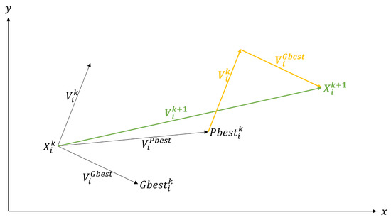
Figure 1.
Search mechanism of the PSO algorithm modified from [24].
3.1.2. EPSO Algorithm
The EPSO (Evolutionary Particle Swarm Optimization) algorithm is a hybrid of the PSO algorithm and evolutionary techniques. According to what was proposed by Vladimiro Miranda, the algorithm consists of the following steps [22,25]:
- Each particle is replicated r times, usually r is equal to 1;
- Parameters A, B, C of expression (30) for the r replicas are mutated;
- The value of the objective function is evaluated for each particle of the new generation;
- Through some selection procedure, the best descendants of each ancestor are selected to form a new generation.
3.1.3. DEEPSO Algorithm
The DEEPSO algorithm is a variation of the EPSO algorithm in which a modified form of the speed Equation (30) shown below is used [22]:
In the expression (33), is given by:
That is to say, is affected by normal noise with average 0 and standard deviation . is a random matrix of ones and zeros, where each element has a 75% probability of being 1 and a 25% probability of being 0 [22].
and are any two points of the population that define four types of implementation of the DEEPSO algorithm that are defined in [22]. For the case of this study, the implementation of the algorithm used was called DEEPSO Pb-rnd, in which and each row of the matrix are chosen from , the particle vector with the best historical values; on the other hand, and for the case of minimization, the following must be fulfilled [22]:
The flow chart for the DEEPSO algorithm implemented to solve the OPF is shown in Figure 2.
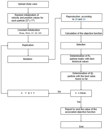
Figure 2.
Flow diagram of the implemented DEEPSO algorithm.
3.2. Genetic Algorithm
The genetic algorithm is a metaheuristic technique initially conceived for solving discrete variable problems. A modification of the genetic algorithm designed to solve continuous variable problems was used for this work [26]. In the following subsections, the implemented genetic algorithm will be described.
3.2.1. Genetic Algorithm Pseudocode
The pseudocode of the genetic algorithm implemented in order to solve the optimal power flow is presented below:
- Generate an initial random population;
- Evaluate the objective function for each element of the initial population;
- Carry out a selection scheme to choose the individuals with the greatest probability of reproduction;
- Recombination of individuals;
- Mutation of individuals;
- Evaluation of the objective function for each element of the new population;
- Selection of the individuals with the best objective function values.
3.2.2. Generation of the Initial Population
To generate the initial population, we proceeded in a similar way to the case of the DEEPSO algorithm, that is, values of variables that met the proposed restrictions were randomly selected.
3.2.3. Evaluation of the Objective Function of the Initial Population
For the genetic algorithm, the implemented objective function, which from now on will be known as the fitness function, is shown in the expression (36):
Thus, if a restriction is violated, the fitness function will assign an infinite value to the cost function, which is known as a penalty.
3.2.4. Selection
For the selection, the tournament scheme was used in references [27,28], in which k groups of m elements were established, where each element m is the value of the objective function associated with a given individual of the population. Since this work seeks to solve a minimization problem, in each group k the m elements are ordered from highest to lowest and a probability of recombination and reproduction is assigned to each element depending on the position they occupy in the array according to the expression (37).
3.2.5. Reproduction and Recombination
For the reproduction phase, two different parents are randomly selected from the entire population according to the reproductive probabilities given in the selection phase. The actual recombination strategy used is shown below, which was taken from [26]. There is a vector , shown in the following expression.
where n is the number of decision variables of the optimization problem. Each value is randomly and uniformly distributed in the interval with . Now, we have the parent vectors x1 and x2 that are shown in the expressions (39) and (40).
Finally, it is clarified that as many parents as elements in the initial population are selected and each pair of parents has a pair of children, so that the new generation (children) has the same size as the initial population and the total population would be twice the size of the initial population size.
3.2.6. Mutation
The mutation takes place for a percentage of individuals of the new generation, that is, not all individuals of the new generation are mutated. For mutated individuals, each variable is modified by adding a normally distributed value with mean 0 and standard deviation .
3.2.7. Evaluation and Selection
For the new generation, the fitness function is assessed. Finally, all the existing particles are ordered, that is, first and second generation from highest to lowest and 50% of the population with the lowest objective function value is selected. This reduces the size of the population to its initial value.
3.2.8. Genetic Algorithm Flow Diagram
The flow chart of the genetic algorithm is shown in Figure 3.
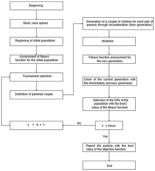
Figure 3.
Flow diagram of the implemented genetic algorithm.
3.3. Analytical Algorithm: Interior Point Method
In this subsection, a description of the interior point method will be presented, since this method was the analytical technique used to solve the optimal power flow in view of its ability to solve non-linear optimization problems. The description presented here is illustrative of the Matpower MIPS solver method [18]. It should be clarified that the solvers used to solve the optimal power flow can use different variations of the method [18,29,30].
The choice of the interior point method is due to a limitation on the part of the software that was used to solve the optimal power flow, since solvers that use Matlab code must be used to implement the non-linear cost functions, its gradients (marginal costs) and its Hessians (derivatives of marginal costs) [18].
3.3.1. Karush–Kuhn–Tucker Conditions
Karush–Kuhn–Tucker conditions are necessary conditions for a point to be a restricted local optimum [31].
If is a local maximum value for the following problem [31]:
The gradients of the constraints at the optimum are independent, then there is a vector such that [31]:
3.3.2. Lagrangian Function
The Lagrangian function is defined as shown below [31]:
3.3.3. MIPS Based Optimization
The optimization problem under study is redefined below [18]:
This optimization problem then becomes a problem where there are only equality restrictions through the inclusion of slack variables Z and the sum of a barrier function to the objective function:
As the perturbation parameter approaches zero, the solution of the previous problem approaches the solution of the original problem. The Lagrangian for a given value of from the previous optimization problem is then:
It should be noted that e is a vector of ones and represents a diagonal matrix with vector A on the diagonal.
To satisfy the Karush–Kuhn–Tucker conditions, the values of and must be found which make expressions (64) to (67) equal to zero as approaches zero. To determine these values, the Newton–Raphson method is used, which produces the following matrix equation:
Since it is possible that the variations , and take the variables to a new infeasible point, they are usually truncated by coefficients as shown below:
There are different ways to determine the values of such as functions of merit, confidence regions, and filtering methods [31]. Finally, the value of must be updated which, as mentioned, should decrease as the number of iterations increases.
4. Results: Optimal Power Flow Solution Considering Heuristic and Analytical Algorithms
For the solution of the optimal power flow consider three test systems: The IEEE system of nine nodes and the IEEE system of 57 nodes. This section shows the results of the optimal power flow solution in each of the aforementioned systems and a validation and comparison of the results obtained by analytical and heuristic methods.
4.1. Nine-Node IEEE System
4.1.1. Nine-Node IEEE System Description
The nine-node system is shown in Figure 4:
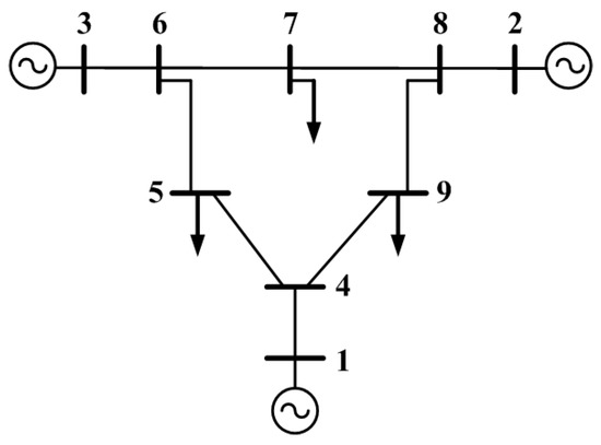
Figure 4.
Nine buses system.
For the case of the nine-node system in the metaheuristic algorithms, five continuous decision variables are used, corresponding to the value of the voltage at the slack node and the active and reactive powers of the other generators different to the slack.
4.1.2. Scenarios Analyzed
Scenario 1
Scenario 1 consists of keeping the generators connected to nodes 1 and 2 as they are established in the original case, that is, with quadratic cost functions; however, the generator connected to node 3 is assumed to be a hydraulic generator with the cost functions defined in [32].
Scenario 2
Scenario 2 now contemplates the connection of a solar plant to node 3, replacing the existing conventional generator. The other generators are not modified.
Scenario 3
In the same way as in scenarios 1 and 2, the conventional generator connected to node 3 is replaced by a wind generator.
Scenario 4
In this scenario, a new controllable load is added to node 5 with a maximum value equal to −30 MW with an average of −19.54 MW and a standard deviation of 0.54 MW.
Table 1, Table 2, Table 3 and Table 4 show the parameters of the renewable generators and the controllable load.

Table 1.
Parameters taken for the cost function of the wind generator.
Table 2.
Parameters taken for the cost function of the run-of-river hydroelectric plant [5].
Table 3.
Parameters taken for the cost function of the solar generator [4].
Table 4.
Parameters taken for the controllable load cost function [4].
4.1.3. Discussion of Obtained Results in the Nine Buses System
The results obtained for all the scenarios in the nine-node system are observed in Table 5, Table 6, Table 7 and Table 8 where the active and reactive power values, the voltage at the slack node, the execution time and the value of the objective function are shown for each optimization technique or solver with which the optimal power flow was solved.
Table 5.
Results obtained for the 9-node system in scenario 1.
Table 6.
Results obtained for the 9-node system in scenario 2.
Table 7.
Results obtained for the 9-node system in scenario 3.
Table 8.
Results obtained for the 9-node system in scenario 4.
It is noteworthy that, for scenario 1, as seen in Table 5, the DEEPSO algorithm yielded a slightly lower value than the analytical solver FMINCON. It is also observed that the analytical solver FMINCON outperforms heuristic algorithms in terms of computation times. On the other hand, it is also observed that the IPOPT and MIPS solvers did not converge for this scenario.
In scenarios 2 and 3 shown in Table 6 and Table 7, the three solvers analyzed reached the local optimum value. The MIPS solver had the best performance in terms of execution time. For the evaluation of the objective function the three solvers reached very similar answers.
In scenario 4, shown in Table 8, the IPOPT solver did not converge, while FMINCON had an excellent performance in terms of computational time. From the analyzed scenarios, the superiority in terms of computation times of the analytical methods with respect to the metaheuristic algorithms is clearly observed.
Although the genetic algorithm converged much faster than the DEEPSO algorithm, the results of the DEEPSO algorithm are much closer to the results obtained by the analytical methods; this is mainly observed in the reactive power values obtained for each generator. It is also observed in the analytical methods that, although the active power values in generators produced by each method are too close to each other, there are small differences in the reactive power values.
4.2. Fifty Seven-Node IEEE System
4.2.1. Fifty Seven-Node IEEE System Description
The IEEE 57-bus test system is used to evaluate the optimization problem of this study. Based on details given in [4] for system buses and branches, the data of the system have been structured in the MATPOWER [6] data format. Branch thermal limits were defined based on reference values given in [5]. A summary of the characteristics of the test system are: seven generators, 42 loads, 63 line/cables, 15 transformers step/wise, two transformers fixed taps and three shunt compensation binary On/Off. Figure 5 below shows the 57-node system on which solar, wind, run-of-the-river generators, controllable loads and batteries were mounted.
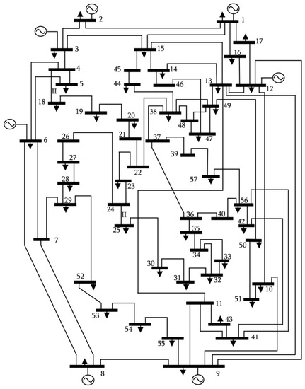
Figure 5.
57 buses system.
4.2.2. Scenarios Analyzed
For the 57-node system, only one scenario was analyzed that took into account all types of generation. It begins by clarifying that for this system the slack node is node 1. The nodes whose generators were changed by generators with uncertain costs are listed below. The nodes to which some type of generation was added and that previously did not have it are also listed.
- The generator connected to node 3 is replaced by a wind generator with uncertain costs;
- The generator connected to node 6 is replaced by a solar generator with uncertain costs;
- The generator connected to node 9 is replaced by a run-of-river hydraulic generator with uncertain costs;
- A battery bank is connected to node 57;
- A controllable charging or electric vehicle charging station is connected to node 47.
The parameters of the cost functions of the generators with cost of uncertainty and of the batteries are shown in Table 9, Table 10, Table 11 and Table 12 (data from previous research: [32]):
Table 9.
Parameters taken for the cost function of the wind generator.
Table 10.
Parameters taken for the cost function of the run-of-river hydroelectric plant [5].
Table 11.
Parameterstaken for the cost function of the solar generator [4].
Table 12.
Parameters taken for the controllable load cost function [4].
Finally, for the battery bank, an operation and maintenance cost is assumed MU/MW.
4.2.3. Discussion of Obtained Results in the 57 Buses System
The results obtained are presented in Table 13, where it is observed that the optimal power flow solution could be found using all optimization techniques. It is also observed that, for the heuristic methods, 17 decision variables are being taken, namely, active and reactive powers in all generators, except for the slack and the voltage of the slack node. Again the interior point method has superiority with respect to the speed of solving the problem, since the metaheuristic techniques took more than 10 min to solve the problem.
Table 13.
Results obtained for the 57 node system.
From the results shown in Table 13, it is possible to see that, as the number of variables in a problem grows, analytical methods have a greater advantage over the heuristics in terms of the speed with which they solve the optimal flow of power and due to the fact that they are not subject to random variation computation of the first iteration of the variable decisions and the computationally high costs for large systems.
It is also observed that the analytical optimum presents a value of the objective function that is lower than that presented by heuristic methods. Furthermore, in this case it is observed that the DEEPSO algorithm does not have such good behavior as to determine the highest value of the objective function, as is observed in the 57 buses system. Additionally, it is also observed that the genetic algorithm has a lower value of the objective function and takes less time than the DEEPSO algorithm. In this way, the appropriate optimization technique for solving the OPF was determined. The inclusion of the cost functions of renewable systems was also considered.
5. Conclusions
In this paper, an optimal power flow was developed that takes into account the uncertainties produced by the penetration of renewable energy sources and controllable loads. It was observed that including the Jacobian (First derivatives) and the Hessian (Second derivatives) of the uncertainty cost functions in the optimal power flow model brings great benefits, since it allows the use of analytical techniques for the determination of active and reactive power dispatches. The main benefit of analytical techniques over the metaheuristic techniques used in the state-of-the-art for the solution of the optimal power flow is the reduction of the computation times that was evidenced in all the cases analyzed, as shown in Table 13. Additionally, it was observed that the IPOPT solver did not converge to a solution in several of the systems and scenarios proposed. On the other hand, the Matlab FMINCON solver converged in all cases to a solution. The MIPS solver did not converge in scenario 1 of the nine-node system.
On the other hand, heuristic methods were used in order to validate the results obtained through analytical methods and very close responses were achieved for the active power dispatches in the IEEE systems of nine and 57 nodes, as shown in Table 5, Table 6, Table 7 and Table 8 and Table 13. However, for the 118-node system, the heuristic methods yielded significantly different dispatch values with respect to the analytical methods; in addition, the dispatches produced by the analytical methods produced a lower value in the objective function. Finally, the presented formulation and its respective solution allow network operators to have a tool to manage the controllable renewable resources found in the network, satisfying the different physical restrictions of the system.
In this way, in this paper the marginal costs of uncertainty are used to determine the active power values that a particular generator with uncertainty must deliver to minimize the uncertainty costs. The field of optimization in electrical power systems is in continuous development. In the case of controllable renewable sources and controllable loads, it is possible to extend this analysis to optimal power flows in DC. It is also possible to use the flow extension optimal power for controllable renewable systems and controllable loads and problems such as Unit Commitment or Security Constraints Optimal Power Flow.
To solve the proposed OPF, when controllable renewable systems and loads are considered, it is also necessary to take into account all the constraints that can affect the power system. The solution would allow the system to work between specified constraints considering uncertainty cost functions, making this problem very complex. Including all constraints in the traditional OPF interior point solution method could prevent convergence and tackling the problem using metaheuristic strategies makes the problem hard to solve within short periods of time (critical clearing times of the contingency in the case of the security constraint optimal power flow) without high computational power.
In this study, the developed research relies on two aspects: the first is analytical methods, using marginal uncertainty cost functions which allow us to use the interior point method for the optimization problem. The second is the solution of the problem using metaheuristic methods, in cases where it is not possible to determine the marginal cost functions. The use of marginal uncertainty cost functions (MUCF) strategies can be employed in small power systems, using strong assumptions of the analytical modeling of cost functions, which makes some of the applications infeasible in real operations or very costly in terms of hardware implementation for real systems. As a solution for those limitations, future research will address the problem using the potential of Parallel and Heterogeneous Computing (PHC).
Author Contributions
Conceptualization, S.R.; Data curation, E.D.R.; Formal analysis, E.D.R. and S.R.; Funding acquisition, S.R.; Investigation, E.D.R. and S.R.; Methodology, E.D.R. and S.R.; Supervision, S.R.; Writing—original draft, E.D.R.; Writing—review & editing, E.D.R. and S.R. All authors have read and agreed to the published version of the manuscript.
Funding
This research received no external funding.
Institutional Review Board Statement
Not applicable.
Informed Consent Statement
Not applicable.
Data Availability Statement
Not applicable.
Acknowledgments
This work was supported by Universidad Nacional de Colombia and Minciencias with project “Programa de Investigación en Tecnologías Emergentes para Microrredes Eléctricas Inteligentes con Alta Penetración de Energías Renovables”, contract No. 80740-542-2020. Additionally, the authors would like to give thanks to: Red Iberoamericana Para el Desarrollo y la Integracion de Pequenhos Generadores Eolicos (MICRO-EOLO) for their support.
Conflicts of Interest
The authors declare no conflict of interest.
References
- UPME. Solicitudes de Conexión de Proyectos de Generación. Available online: https://www.grupoenergiabogota.com/transmision/nosotros/solicitudes-de-conexion-de-generacion (accessed on 24 August 2021).
- Jordehi, A.R. How to deal with uncertainties in electric power systems? A review. Renew. Sustain. Energy Rev. 2018, 96, 145–155. [Google Scholar] [CrossRef]
- Hetzer, J.; Yu, D.C.; Bhattarai, K. An economic dispatch model incorporating wind power. IEEE Trans. Energy Convers. 2008, 23, 603–611. [Google Scholar] [CrossRef]
- Arevalo, J.; Santos, F.; Rivera, S. Uncertainty cost functions for solar photovoltaic generation, wind energy generation, and plug-in electric vehicles: Mathematical expected value and verification by Monte Carlo simulation. Int. J. Power Energy Convers. 2019, 10, 171–207. [Google Scholar] [CrossRef]
- Molina, F.; Perez, S.; Rivera, S. Formulación de funciones de costo de incertidumbre en pequeñas centrales hidroeléctricas dentro de una microgrid. Ing. USBMed 2017, 8, 29–36. [Google Scholar] [CrossRef]
- Bernal, J.; Neira, J.; Rivera, S. Mathematical uncertainty cost functions for controllable photo-voltaic generators considering uniform distributions. WSEAS Trans. Math. 2019, 18, 137–142. [Google Scholar]
- Vargas, S.; Rodriguez, D.; Rivera, S. Mathematical formulation and numerical validation of uncertainty costs for controllable loads. Rev. Int. Métodos Numéricos Calculo Diseño Ing. 2019, 35. [Google Scholar] [CrossRef]
- Martinez, C.; Rivera, S. Modelación cuadrática de costos de incertidumbre para generación renovable y su aplicación en el despacho económico. Rev. MATUA 2018, 5, 2389–7422. [Google Scholar]
- Arévalo, J.; Santos, F.; Rivera, S. Application of analytical uncertainty costs of solar, wind and electric vehicles in optimal power dispatch. Ingenieria 2017, 22, 324–346. [Google Scholar] [CrossRef]
- Li, P.; Zhou, Z.; Shi, R. Probabilistic optimal operation management of microgrid using point estimate method and improved bat algorithm. In Proceedings of the 2014 IEEE PES General Meeting | Conference Exposition, National Harbor, MD, USA, 27–31 July 2014; pp. 1–5. [Google Scholar] [CrossRef]
- Zhao, J.; Wen, F.; Dong, Z.Y.; Xue, Y.; Wong, K.P. Optimal dispatch of electric vehicles and wind power using enhanced particle swarm optimization. IEEE Trans. Ind. Inform. 2012, 8, 889–899. [Google Scholar] [CrossRef]
- Rivera, S.; Torres, J. Optimal energy dispatch in multiple periods of time considering the variability and uncertainty of generation from renewable sources/Despacho de energía óptimo en múltiples periodos de tiempo considerando la variabilidad y la incertidumbre de la generación a partir de fuentes renovables. Prospectiva 2018, 16, 75–81. [Google Scholar]
- Guzman, W.; Osorio, S.; Rivera, S. Modelado de cargas controlables en el despacho de sistemas con fuentes renovables y vehículos eléctricos. Ing. Reg. 2017, 17, 49–60. [Google Scholar] [CrossRef][Green Version]
- Peña, A.; Romero, D.; Rivera, S. Generation and demand scheduling in a micro-grid with battery-based storage systems, hybrid renewable systems and electric vehicle aggregators. WSEAS Trans. Power Syst. 2019, 10, 8–23. [Google Scholar]
- Torres Riveros, J.; Rivera, S. Despacho de energía óptimo en múltiples periodos considerando la incertidumbre de la generación a partir de fuentes renovables en un modelo reducido del sistema de potencia colombiano. Av. Investig. Ing. 2018, 15, 48–58. [Google Scholar] [CrossRef]
- UPME. Plan de Expansión de Generación-Transmisión 2017–2031. Available online: https://www.acolgen.org.co/estudio-servicios-complementarios-2/ (accessed on 24 August 2021).
- Gomez-Exposito, A.; Conejo, A.; Canizares, C. Electric Energy Systems: Analysis and Operation; Electric Power Engineering Series; CRC Press: Boca Raton, FL, USA, 2017. [Google Scholar]
- Zimmerman, R.D.; Murillo-Sánchez, C.E. MATPOWER User’s Manual. Available online: https://matpower.org/docs/MATPOWER-manual.pdf (accessed on 24 August 2021).
- Stevenson, J.J.G.W.D. Análisis de Sistemas de Potencia. Available online: https://ingenieria.udistrital.edu.co/course/view.php?id=1408 (accessed on 24 August 2021).
- Wen, Y.; Guo, C.; Pandžić, H.; Kirschen, D.S. Enhanced security-constrained unit commitment with emerging utility-scale energy storage. IEEE Trans. Power Syst. 2016, 31, 652–662. [Google Scholar] [CrossRef]
- Pozo, D.; Contreras, J.; Sauma, E.E. Unit commitment with ideal and generic energy storage units. IEEE Trans. Power Syst. 2014, 29, 2974–2984. [Google Scholar] [CrossRef]
- Miranda, V.; Alves, R. Differential Evolutionary Particle Swarm Optimization (DEEPSO): A Successful Hybrid. In Proceedings of the 2013 BRICS Congress on Computational Intelligence and 11th Brazilian Congress on Computational Intelligence, Ipojuca, Brazil, 8–11 September 2013; pp. 368–374. [Google Scholar] [CrossRef]
- Kennedy, J.; Eberhart, R. Particle swarm optimization. In Proceedings of the ICNN’95-International Conference on Neural Networks, Perth, WA, Australia, 27 November–1 December 1995; Volume 4, pp. 1942–1948. [Google Scholar] [CrossRef]
- Alam, M. Particle swarm optimization: Algorithm and its codes in matlab. ResearchGate 2016, 8, 1–10. [Google Scholar] [CrossRef]
- Arevalo, J.; Medina, D.; Rueda, J.; Rivera, S. 2018 competition on operational planning of sustainable power systems: Testsbeds and results. WSEAS Trans. Power Syst. 2019, 14, 98–106. [Google Scholar]
- Mostapha Kalami, H. Practical Genetic Algorithms in Python and MATLAB—Video Tutorial. Available online: https://www.udemy.com/course/genetic-algorithms-in-python-and-matlab/ (accessed on 24 August 2021).
- Goldberg, D.; Deb, K. A comparative analysis of selection schemes used in genetic algorithms. FOGA 1990, 1, 69–93. [Google Scholar]
- Miller, B.; Goldberg, D. Genetic algorithms, tournament selection, and the effects of noise. Complex Syst. 1995, 9, 193–212. [Google Scholar]
- Wang, H.; Murillo-Sanchez, C.E.; Zimmerman, R.D.; Thomas, R.J. On computational issues of market-based optimal power flow. IEEE Trans. Power Syst. 2007, 22, 1185–1193. [Google Scholar] [CrossRef]
- Wächter, A.; Biegler, L.T. On the implementation of an interior-point filter line-search algorithm for large-scale nonlinear programming. Math. Program. 2006, 106, 25–57. [Google Scholar] [CrossRef]
- Parkinson, A.R.; Balling, R.; Hedengren, J. Optimization Methods for Engineering Design, 2nd ed.; Brigham Young University: Provo, UT, USA, 2018. [Google Scholar]
- Reyes, E.D.; Bretas, A.S.; Rivera, S. Marginal uncertainty cost functions for solar photovoltaic, wind energy, hydro generators, and plug-in electric vehicles. Energies 2020, 13, 6375. [Google Scholar] [CrossRef]


Publisher’s Note: MDPI stays neutral with regard to jurisdictional claims in published maps and institutional affiliations. |
© 2021 by the authors. Licensee MDPI, Basel, Switzerland. This article is an open access article distributed under the terms and conditions of the Creative Commons Attribution (CC BY) license (https://creativecommons.org/licenses/by/4.0/).