Abstract
The use of distribution-based data representation to handle large-scale scientific datasets is a promising approach. Distribution-based approaches often transform a scientific dataset into many distributions, each of which is calculated from a small number of samples. Most of the proposed parallel algorithms focus on modeling single distributions from many input samples efficiently, but these may not fit the large-scale scientific data processing scenario because they cannot utilize computing resources effectively. Histograms and the Gaussian Mixture Model (GMM) are the most popular distribution representations used to model scientific datasets. Therefore, we propose the use of multi-set histogram and GMM modeling algorithms for the scenario of large-scale scientific data processing. Our algorithms are developed by data-parallel primitives to achieve portability across different hardware architectures. We evaluate the performance of the proposed algorithms in detail and demonstrate use cases for scientific data processing.
1. Introduction
Thanks to the power of modern supercomputers, scientists in various fields can use computer programs to simulate real-world phenomena with higher resolution. In addition, the development of data analysis and visualization technology has also helped these scientists to understand such datasets better. With the increasing size of scientific datasets, the challenges of analysis and visualization tasks continue to grow. The classic data analysis and visualization workflow needs to write the raw data produced by the simulation into the hard disk first and then conduct subsequent analysis. This workflow will suffer from storage space limitations and I/O bottlenecks if the dataset size is huge. Therefore, scientists are currently more inclined to process the scientific data in situ [1,2] while the data is still in the supercomputer’s memory. The primary purpose of the in situ workflow is to keep only the crucial information for data analysis and reduce the size of data to be written to the hard disk. Although many techniques can reduce the size of datasets, such as subsampling, lossy compression, etc., distribution-based data representation [1,3,4] is an emerging method of handling the large-scale scientific data problem, which can not only compactly represent the dataset, but also retain important statistical characteristics to facilitate data analysis tasks.
It is commonly agreed that distribution modeling is a time-consuming task when modeling distribution from a huge amount of samples. It is imperative to parallelize the distribution-fitting process and fully utilize the supercomputer’s power, as its use time is costly. Although many parallel single-distribution fitting algorithms have been proposed [5,6,7], these algorithms focus on modeling single distribution from a huge amount of input samples. For distribution-based scientific data modeling, a dataset is often transformed into multiple distributions and each distribution is calculated from a small number of samples. A classic example is to represent an ensemble dataset [8] by distributions. In an ensemble dataset, simulation produces hundreds to thousands of data values at each spatial location, and scientists are usually interested in studying the statistical characteristics in different spatial regions. If representing an ensemble dataset whose spatial resolution is and the sample count at each spatial location is 100, we have to model distributions, each of which is calculated from just 100 samples. Therefore, the parallel single-distribution fitting algorithms cannot fit the scenario of scientific data modeling well because they could lead to insufficient parallelism, and they still do not maximize the use of the supercomputer’s resources.
In this paper, we propose parallel algorithms for distribution-based scientific data modeling. We develop our algorithms based on data-parallel primitives, because many such frameworks have been proposed, such as Thurst [9], VTK-m [10], and PISTON [11], and algorithms implemented by these frameworks can be portable across different computing backends, such as GPUs and multi-core CPUs. Some supercomputer systems are heterogeneous clusters, such as the Darwin cluster in Los Alamos National Laboratory, in which different nodes may be equipped with different computing hardware. Our data-parallel primitive-based algorithms can facilitate the data process that is run on supercomputers with different types of computing nodes. In this work, we propose parallel multi-set distribution modeling algorithms for multi-variant histogram [3,12,13,14,15] and GMM [1,2,4,15,16,17] modeling, because these are the most popular non-parametric and parametric distribution representations in the scientific data modeling, respectively.
The rest of the paper is organized as follows. Section 2 discusses related work about distribution data processing techniques, parallel distribution modeling works, and data-parallel primitives. Section 3 briefly introduces the data format of scientific datasets and the popular distribution-based approaches for handling large-scale scientific datasets, and defines the data-parallel primitives we will use to design our proposed algorithms. The proposed histogram modeling and GMM modeling algorithms are introduced in Section 4 and Section 5, respectively. Section 6 shows the performance of the proposed algorithms, the influence of parameters, and the scalability using multiple scientific datasets. Section 7 demonstrates the use case of the proposed algorithms on scientific data processing and analysis. Section 9 discusses the pros and cons of our approach by comparing with other parallel options. Section 8 concludes this paper and discusses future work.
2. Related Work
2.1. Distribution-Based Large Data Processing and Analysis
Many distribution-based approaches have been proposed to handle, analyze, and visualize large-scale scientific datasets. Liu et al. [16] modeled ensemble data into several GMMs, and then used specific methods to convey the uncertainty. Li et al. [8] modeled the particle data using several multivariant GMMs after partitioning the dataset and then found the partitions with poor modeling quality to optimize. Thompson et al. [3] approximated the topological structure and fuzzy isosurface by partitioning the data into several histogram representations. Dutta et al. [1,2,18] used GMM to represent datasets compactly in an in situ environment. Furthermore, Wang et al. [4,15,19] used distributions to compactly store volume, time-varying, ensemble datasets for the post-hoc data analysis and visualization. Chaudhur et al. [20,21] and Lee et al. [12] employed distribution to conduct efficient data query and visualization. Wei et al. [13,14] used bitmap index to efficiently support both single and multivariant distribution queries for data analysis. Chen et al. [22] applied Gaussian distribution to model the uncertainty of the pathline in time-varying flow field datasets. Thus, even if the purposes of the applications are different, it is certain that modeling several distributions is indeed a frequently used technique for scientific data processing and reduction.
2.2. Parallelization of Modeling Distribution
Many parallel algorithms have been proposed to model single distribution from a huge amount of input samples. Kumar et al. [5] used CUDA to parallelize GMM modeling on the GPU. Kwedlo et al. [6] proposed an algorithm for parallel modeling of GMM on NUMA systems using OpenMP. Shams et al. [7] employed CUDA to parallelize the calculation of a histogram on the GPU. These algorithms focus on developing algorithms for specific hardware (CPU or GPU) to provide efficient distribution computation. However, they only consider single distribution modeling. Hence, these parallel algorithms cannot fully utilize the hardware resources and provide good performance when we seek to model multiple distributions from multiple small sample sets concurrently.
2.3. Data Parallel Primitives
It has been more than 30 years since Blelloch [23] proposed the parallel vector model, which treats a vector as a whole to be operated. With the development of this concept, data-parallel primitives(DPP) became a choice for parallel computing. For those algorithms that are suitable for vectorization, parallelization through DPP can achieve better acceleration results. In the application of optimizing probabilistic graphical models, Lessley et al. [24] found that DPP has a better acceleration performance than OpenMP.
DPP does not only accelerate computation, it also achieves cross-platform capability through encapsulation. For example, NVIDIA’s Thrust [9] and VTK-m [10] are libraries that provide several DPPs which can be compiled on multiple platforms. Many previous studies are devoted to hardware optimization when parallelizing certain algorithms on specific systems. Austin et al.[25] proposed a distributed memory parallel implementation of Tucker decomposition. Hawick et al.[26] proposed a distributed parallel algorithm for geographic information systems. The above research focuses on the underlying differences in memory access time or data communication time caused by different implementation methods of specific hardware. DPP can help us save the time of optimizing specific hardware implementations and provide good portability. Yenpure et al. [27] used DPP to deal with the problem of point merging. Larsen et al. [28] proposed a volume rendering algorithm based on DPP, which can support cross-platform execution. Lessley et al. [29] proposed a cross-platform hash table and conflict resolution method. Li et al. [30] used wavelet compression to solve the problem of IO bottlenecks caused by excessive datasets and achieved cross-platform advantages through DPP. In addition, Lessley et al. [31] proposed an algorithm based on DPP to solve the maximal clique enumeration problem. The DPP-based algorithms have comparable performance to parallel algorithms designed for specific platforms and even better portability. Therefore, users only have to write the code once using data-parallel primitives and can run the parallel programs on different computing backends by simply changing the complication options. DPP allows users to focus on the development of high-level algorithms without worrying about the underlying optimization, or even portability. This significantly reduces the programming time. In addition, the above algorithms are designed to solve problems in different fields, which also demonstrates that DPP can be used to develop parallel versions of various algorithms.
3. Background
3.1. Scientific Dataset
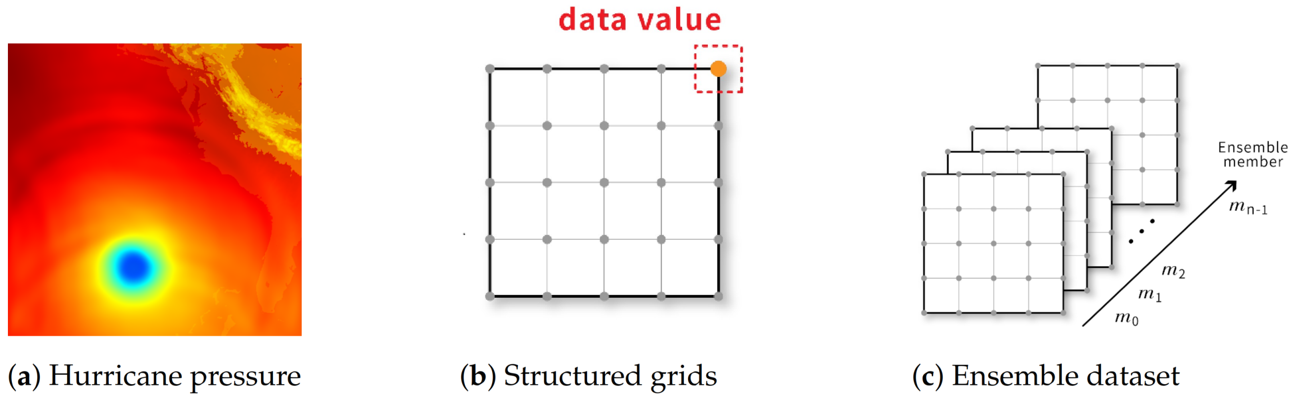
Scientific data are records of the observation or simulation of phenomena that occur in nature. To store the data from the continuous spatial space in a file, we usually decouple the data into attributes and the domain structure. Figure 1a,b show an example of a scientific dataset, with its domain structure and attributes. The domain structure describes the topological structure of a scientific dataset, which specifies the relationship among locations for storing data values. The attributes are the data values obtained from simulation or observation at grid points. The data value at a grid point could be a scalar or a vector. If grid points in a scientific dataset are arranged in a regular grid, this scientific dataset is called a structured grid dataset. Because the arrangement is regular, each grid point can be indexed through (i, j) in 2D or (i, j, k) in 3D, etc. The grid points can have many different appearances. In this paper, we will focus on the datasets stored by the simplest structured grid illustrated in Figure 1b. If a dataset stores data values in the spatial space and the data value at each grid point is a scalar value, we call it a volume dataset. If the data value on each grid point is a vector, we call it a vector dataset. If each grid point stores multiple data values and each data value comes from a simulation run, we call the dataset an ensemble dataset, and the data from one simulation run is called an ensemble member. We illustrate the ensemble dataset in Figure 1c.

Figure 1.
(a) is the visualization of a 2D slice of a 3D hurricane pressure dataset; (b) is the illustration of the corresponding grid structure of (a) and the pressure values are stored at grid points; (c) is an illustration of an ensemble dataset. In this example, we have n ensemble members and each ensemble member is a volume data or vector data from the same simulation.
3.2. Distribution-Based Scientific Data Modeling
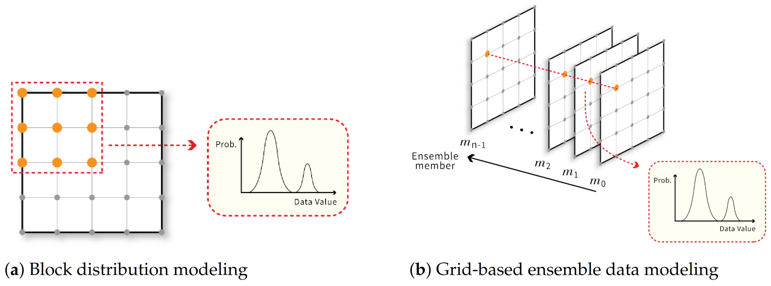
A dataset could be enormous if the spatial resolution of the volume dataset and vector dataset, or the number of members of the ensemble dataset, is large. When the dataset size increases, data I/O and analysis time will increase and obstruct the data analysis pipeline. One of the most popular approaches for handling large scientific datasets is to model datasets using distributions. For example, Dutta et al. [1] and Thompson et al. [3] divided a volume dataset into sub-blocks, where data values of each sub-block are stored by a univariant GMM or histogram when the spatial resolution of the dataset is huge. Li et al. [17] used the same idea to model vectors in a sub-block with a multivariant GMM to store the vector dataset compactly. Figure 2a illustrates the above ideas. This distribution-based approach reduces the data size and preserves the statistical characteristics to support the post-hoc analysis task more accurately. Another example is that scientists are usually interested in analyzing the statistical characteristics across all members in the ensemble dataset instead of individual members. Liu et al. [16] modeled data values at each grid point in an ensemble data using a univariant GMM and store. This compact distribution representation reduces the storage requirement, and the statistical characteristics can still be visualized in the post-hoc analysis stage. Figure 2b illustrates this distribution-based ensemble data representation. More sophisticated distribution-based representations for scientific datasets have been proposed, as discussed in Section 2.1.
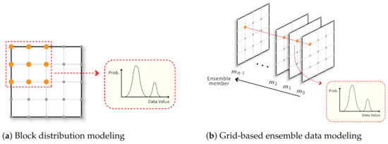
Figure 2.
(a) illustrates the approach that uses a distribution to model data values in each sub-block to compactly represent a volume or vector dataset. If the data is a vector dataset, the distributions should be multivariant distributions; (b) shows the use of a distribution to model data values of all ensemble members at the same grid point to compactly store an ensemble dataset.
3.3. Data Parallel Primitives
In this paper, we use parallel data primitives to parallelize the algorithms for histogram and GMM modeling. To form the basic units of parallelized algorithms, various algorithms can be produced through the permutations and combinations of many DPPs. In this section, we will briefly introduce a few DPP functions used in this paper.
Map receives N arrays with length K and an operator as arguments, and it returns M arrays of length K. N and M are determined by the operators in the parameters. Map will map the input arrays to output arrays by running the input operator on each element independently. For example, C=MAP(A,B,operator=Add()) will compute C[i]=A[i]+B[i] for all elements. Map primitive and user-defined operators are generally used to replace the traditional loop procedure.
Reduce receives an array and an operator as arguments and returns an output value. REDUCE builds a merge tree and uses multiple threads to merge all elements of the input array into a final output at the same time through the input operator. For example, C=REDUCE(A, operator=ADD()) will add all values together and store the result in C. ReduceByKey is similar to REDUCE, but needs an additional key array with the same length as the input array. ReduceByKey merges values in the input array which have the same corresponding elements in the key array into a single value using the operator. If the key array has N unique values, the length of the output array should be N.
Gather receives an array A of length N and an index array B of length M, and returns an array C of length M. For each element in array B, Gather copies the value in array A to .
4. Histogram Modeling Using Data-Parallel Primitives
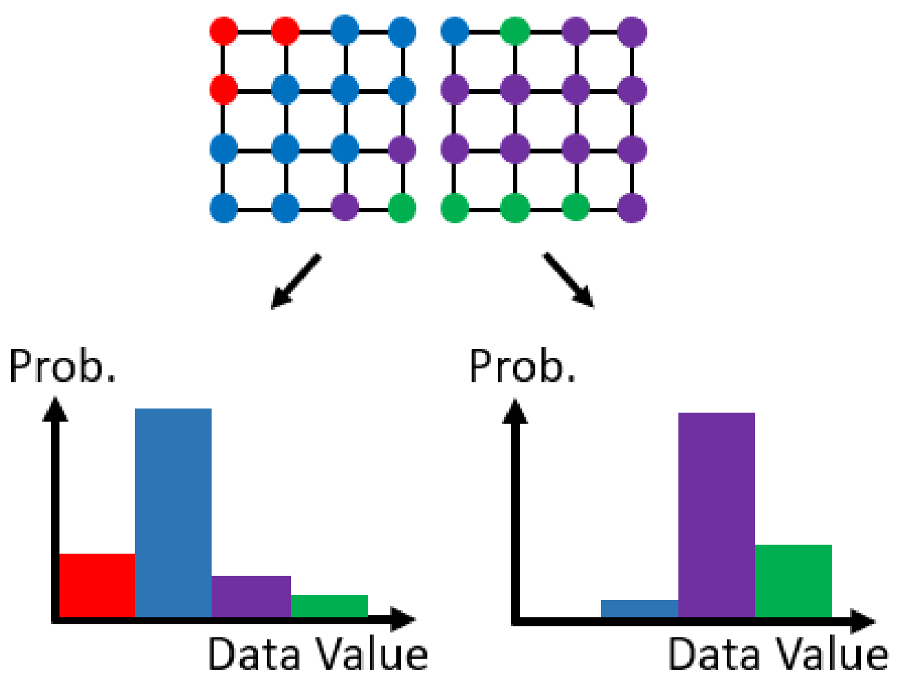
The histogram [32,33] is a popular non-parametric distribution representation which has been widely used in many fields [3,15,34,35,36]. A histogram divides the data value domain into bins and calculates the number (frequency) of input samples that belong to each bin. If the input samples are single-variant, the histogram contains pairs of bin index and frequency, , where B is the number of desired bins. If the input samples are multi-variant, the histogram also shows pairs of bin index and frequency. The major difference is that in the multi-variant histogram consists of multiple indices, according to the number of variables of input samples. When modeling multi-variant data using the histogram, the number of bins of the histogram is where is the number of bins of variable. The number of bins is large, so that the frequencies of many bins may be 0. Therefore, a sparse histogram representation, which does not store the bins with 0 frequency, is often used to save the storage. This section will introduce the algorithm to calculate multiple histograms using data-parallel primitives. Each histogram is computed from a set of input samples. Figure 3 is an example of modeling a scientific dataset using histograms. The resolution of the dataset is 8 × 4 and it is divided into two 4 × 4 sub-blocks (sets) to calculate two histograms. We first introduce the serial version of a multi-set histogram modeling algorithm, then introduce the parallel version algorithm using data-parallel primitives.
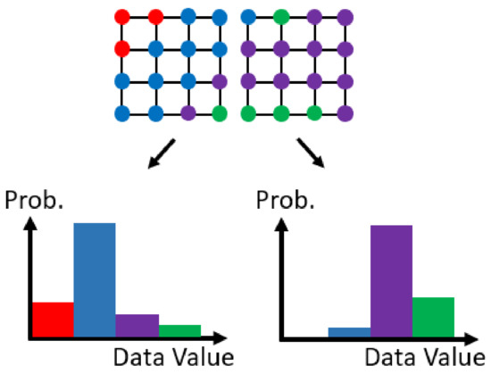
Figure 3.
An example of dividing a scientific dataset into two sets and transforming the data values in each set into a histogram.
Algorithm 1 is the pseudo-code of the serial version of the multi-set histogram modeling algorithm. respectively uses , and to represent the number of sets, the number of samples in each set, and the number of variables of all the samples. is an array whose length is the same as the number of variables. Each element of stores the number of bins of the corresponding variable.
is the output array to store multi-set histograms. The length of is the total number of sets, and each element is a dictionary to store a histogram of samples of a set. This algorithm first calculates the of all samples and the of the corresponding variable. stores the value range of each variable of all samples. stores the value interval of a bin of each variable. Then, we use the interval to calculate the bin indices for all samples. The following two main steps are used to compute the histograms:
- Use each bin interval in to compute the bin index of the corresponding variable of the samples (Lines 9–11).
- The sample’s bin indices of all variables are used as the key of the dictionary to accumulate the number of occurrences of the key (Line 12).
Dictionary (Line 7) is used to store the histogram of a set. Each item of a dictionary has a key/value pair. The key is a combination of bin indices of all variables. The value is the frequency of the corresponding bin indices. The get function at Line 12 returns the value of a key. If the key does not exist, the get function returns the default value, 0. We use the dictionary because we can use sparse representation to avoid storing large amounts of bins with zero frequency.
| Algorithm 1 Serial Version of the Multi-set Histogram Algorithm |
|
Algorithm 2 is the DPP version algorithm. At the top of the algorithm, there are five input arrays and two output arrays. stores all samples from all sets. stores the set ID of the corresponding element in so the lengths of and are the same. Each element of stores the number of desired bins of the corresponding variable. and are the maximal and minimal values of the variable. We then model the input samples with the same set ID into one histogram. The lengths of the output array and are M, which is determined by the total number of non-zero frequency bins. An element of stores the set ID and multi-variant index of a bin. The corresponding element of stores the frequency the bin.
| Algorithm 2 DPP Version of the Multi-set Histogram Modeling Algorithm |
|
The main purpose of computing multi-set histograms is to determine the number of samples whose set ID and multi-variant bin index are the same. To achieve this purpose in parallel, we can divide the process into the following three main steps:
- Calculate the multi-variant bin index of all samples in parallel (Line 10).
- Use 1D index to encode the set ID and multi-variant index of a sample (Line 11).
- Count the the number of samples whose 1D indices are the same (Line 14).
The idea of the second step is the same as converting the index of a multi-dimensional array into a 1D index. This calculation is completed by the operator at Line 11 using Equation (1).
stores the 1D indices of all samples and is used as the key in ReduceByKey at Line 14 to compute the number of samples whose 1D indices are the same. The major advantage of using the 1D index as the key to execute the ReduceByKey is that most of the data-parallel primitives libraries implement ReduceByKey by using scalar values as the key. At Line 15, we get unique indices and store them in . The length must be the same as . Finally, we compute from through operator . is the reversed process of , which converts the 1D index back to the set ID and multi-variant index.
5. Gaussian Mixture Model Modeling Using Data-Parallel Primitives
The Gaussian Mixture Model is a parametric distribution representation. It can represent a complicated distribution using a few parameters to provide a compact and accurate distribution representation. Therefore, GMM has been widely used to facilitate scientific data reduction and visualization [2,8,17,18,19,37,38].
GMM is an extension of a single Gaussian distribution; it is a statistical model that decomposes the distribution of samples into the weighted sum of K Gaussian distributions. GMM expresses the weighted sum of these K Gaussian components by Equation (2).
where x is the D-variant sample, is the weight of the Gaussian component, and , is the probability density of x on the D-variate Gaussian distribution with the mean vector, , and the covariance matrix, . The definition of is represented by Equation (3), which is called the parameter set of the Gaussian Mixture Model.
The expectation-maximization (EM) algorithm is generally used to estimate parameters of a GMM of the given samples. The EM algorithm estimates the parameters by maximizing the following likelihood function through an iterative process:
where represents the parameters of GMM and is the input sample. K is the number of Gaussian components. , , and represent the weight, mean vector, and covariance matrix of the Gaussian component, respectively.
Algorithm 3 is the pseudo code of the serial version of the multi-set EM algorithm for GMM modeling. Each set of input samples will be modeled by a GMM. The input array, , contains samples from all sets. As the input samples could be multi-variant, an input sample, , is a vector whose length is determined by the number of variables of the input dataset. is all input samples of set and is the total number of input samples of the set. The loop at Line 5 iterates through each set to fit the samples to a GMM with K Gaussian components.
| Algorithm 3 Serial Version of the Multi-set EM Algorithm |
|
In the initialization step, we set the responsibilities between all input samples and Gaussian components. The responsibilities are stored in the array. can be interpreted as the probability that the is generated by the Gaussian component. Therefore, responsibilities between sample and all Gaussian components must satisfy . will be updated through the EM algorithm and used to update the parameters of GMMs. The EM algorithm will iterate the following three steps to update , and thereby estimate the parameters of GMM of each set:
- M-step: use the current to estimate the parameter (Line 10).
- E-step: compute the maximum likelihood of current GMM, and update responsibilities between all samples and current Gaussian components of the corresponding GMM, and store responsibilities in (Line 31).
- Check whether the maximum likelihood has converged (Line 48).
When the algorithm is finished, the estimated weights, mean vectors, and covariance matrices of all GMMs are stored in , , and , respectively.
5.1. Input and Output Arrays
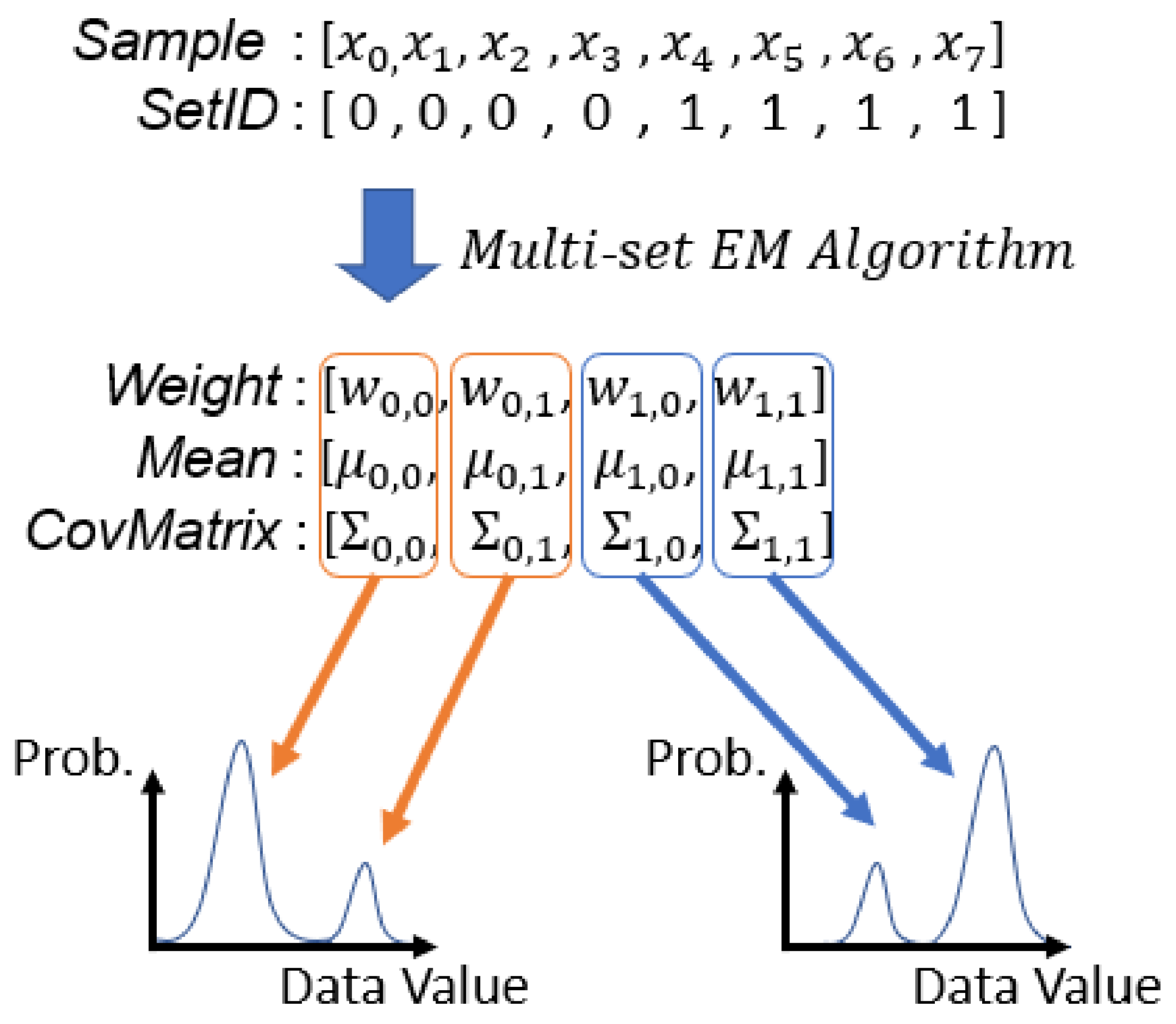
In this section, we introduce the proposed Data-Parallel Primitive (DPP) version of the multi-set EM algorithm. We first introduce the format of input and output arrays in the DPP version algorithm (Algorithm 4). Figure 4 is an example of input and output arrays. Our goal is to compute multiple EM results from multiple sets of samples concurrently using data-parallel primitives. A GMM is used to model samples of a set. The number of input samples of each set could be different and the samples might be multi-variant samples. All GMMs produced by our algorithm have the same number of Gaussian components (K). We then flatten most of the arrays in the DPP version algorithm, because flat arrays are easier to process with data-parallel primitives, to maximize the parallelization.
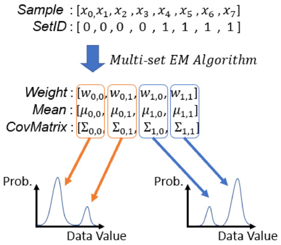
Figure 4.
Examples of input and output arrays of running EM algorithm with two sets of samples when the number of Gaussian components (K) of each GMM is 2. In this example, to are all in the first set and to are in the second set. , and are the parameters of the Gaussian component in the set.
All the input samples are stored in an 1D array . is an array whose length is the same as that of . Each element of stores the set ID of the corresponding sample in . , , and store the parameters of GMMs of all sets. As all GMMs have the same number of Gaussian components, the length of , , and is , where S is the total number of sets and K is the number of Gaussian components of a GMM. These three arrays respectively store the , and of each Gaussian component, which are the parameters of GMM. , , and , respectively, represent , and of the Gaussian component in the set.
is an array that stores all responsibilities between samples and the Gaussian components of the corresponding GMM. So, the size of is where is the number of input samples of the set and N is the total number of input samples. In the algorithm of GMM modeling, is an important array which is used to estimate new parameters of GMMs, and is also updated by GMMs and input samples. The values of at Line 8 of Algorithm 3 are randomly set. A responsibility in is computed from a sample and a Gaussian component which consists of a weight, mean vector, and a covariance matrix. The elements in and are indices of the sample and the Gaussian component, respectively, used to compute the corresponding responsibility, respectively. These arrays are used to assist our parallel algorithm to complete multiple tasks using data-parallel primitives, such as computing array from , , , and . The details will be introduced in the following sections.
| Algorithm 4 DPP Version of the Multi-set EM Algorithm |
|
5.2. M-Step
In this step, three parameters, , and , of all Gaussian components are estimated from and concurrently. The aim is to duplicate the array to create proper pairs between responsibilities and samples, and use data-parallel primitives to compute the information we need.
5.2.1. Weight Estimation
In general, the Gaussian component’s weight represents the Gaussian component’s contribution in the GMM, or the weight of a Gaussian component can be interpreted as how much ratio of input samples can be drawn from the Gaussian component.
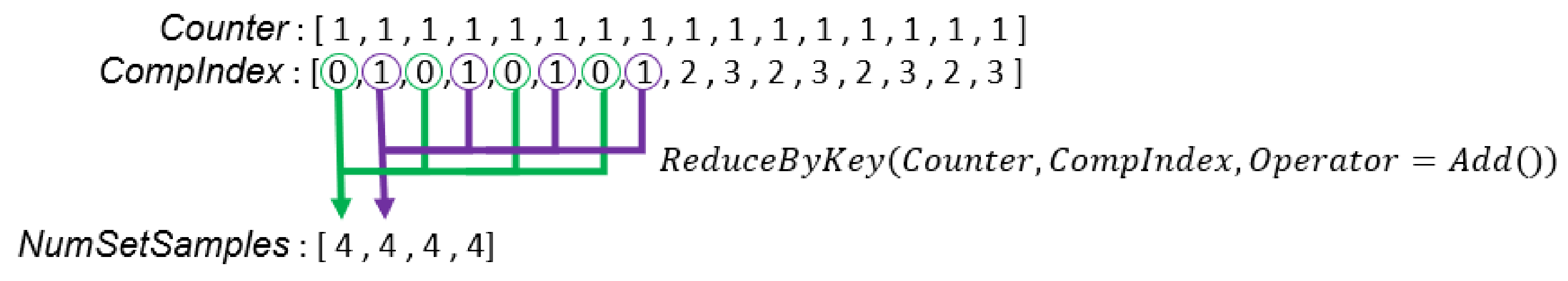
To calculate the weights of all Gaussian components from all sets, we should use data-parallel primitives to add up responsibilities that belongs to the same Gaussian. To achieve this goal, we prepare an array, , whose length is the same as array. Values in indicate the Gaussian component ID of the corresponding value in array. The component ID of a Gaussian component is unique among Gaussian components of all GMMs. Then, we can use the ReduceByKey primitive to compute non-normalized weights of all Gaussian components from all sets (Line 16 in Algorithm 4). We illustrate this process in Figure 5. To normalize the weights, we use the MAP primitive to divide each weight by the number of samples in the set (Line 17 in Algorithm 4). Figure 6 illustrates how to calculate for the weight normalization.
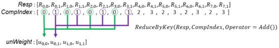
Figure 5.
In this example, there are two sets of samples, and each GMM has two Gaussian components. is the probability that the is generated by the Gaussian component. is the non-normalized weight of the Gaussian component in the set.
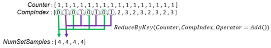
Figure 6.
The generation process of .
5.2.2. Mean Vector Estimation
At Line 21 in Algorithm 3, the loop shows the procedure of the serial algorithm to estimate new mean vectors, , of a GMM. In this step, mean vectors are computed from the responsibilities (), the non-normalized weight (), and input samples ().
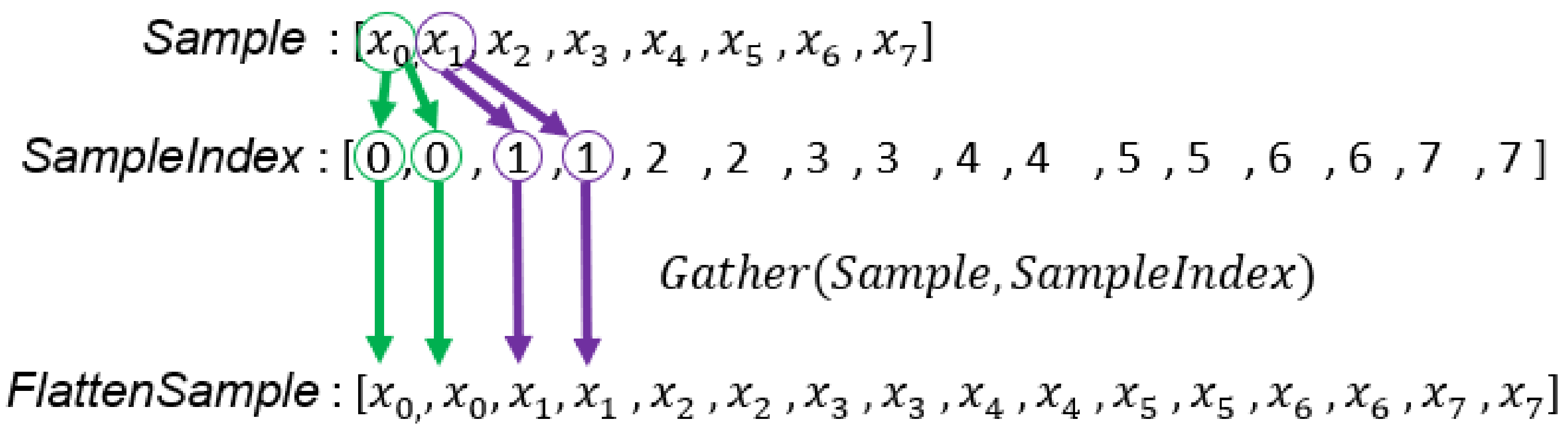
From Lines 19–23 in Algorithm 3, we know that in order to compute mean vectors of a GMM with K Gaussian components, an input sample will be accessed K times. To use the data-parallel primitives to complete this calculation, we duplicate the array so that the length of the duplicated array is the same as the array. To achieve this goal, we need the array; this has a length of . The content consists of all indices of the array repeated K times. Figure 7 illustrates the procedure that uses to create a duplicated sample array, . We only create once before the main loop of the EM algorithm because input samples never change (Line 10 in Algorithm 4). Then, we can apply the Map and ReduceByKey primitives to calculate the mean vectors of all GMMs concurrently. Figure 8 illustrates the computation of the mean vectors, which corresponds to Lines 19 to Line 21 in Algorithm 4.
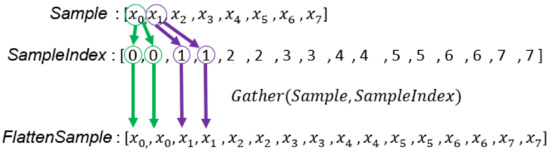
Figure 7.
The generation process of . For example, is copied twice because each GMM has two Gaussian components and each sample will be accessed to compute .
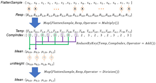
Figure 8.
The computation process of . is a responsibility computed from the sample and Gaussian component. is the mean vector of the Gaussian component in the set.
5.2.3. Covariance Matrix Estimation
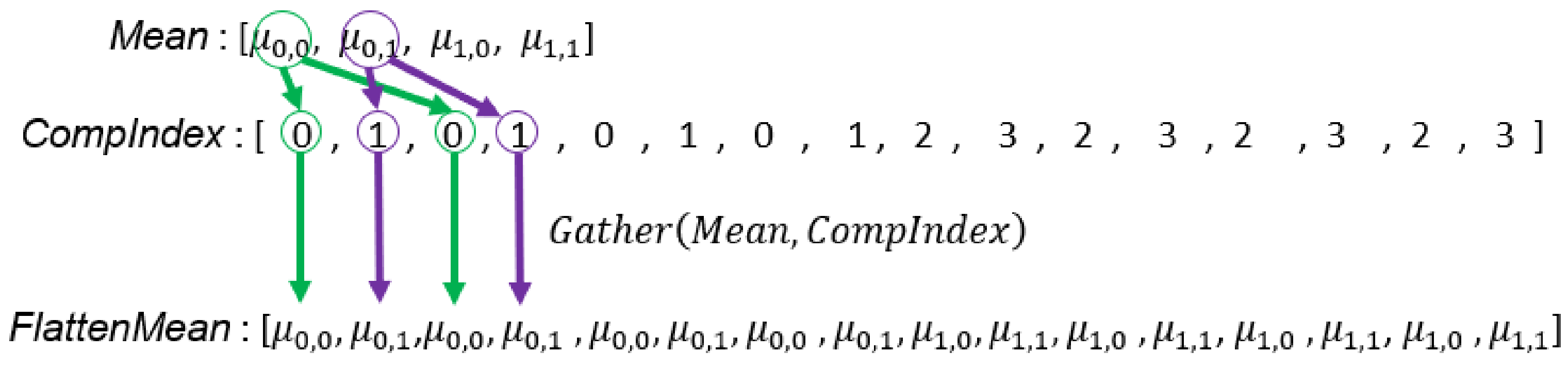
Line 5 and Lines 25–27 in Algorithm 3 compute the differences between a sample and all mean vectors in the corresponding set. The corresponding code segment in the DPP version algorithm is Lines 10, 23, and 24 in Algorithm 4. To parallelize this operator using data-parallel primitives, we need two arrays that store all combinations of samples and mean vectors to compute in parallel. These two arrays store duplicated samples: , introduced in Section 5.2.2 and duplicated mean vectors, , produced by Line 23 in Algorithm 4, where is the predefined array used to correctly produce . Figure 9 and the top part of Figure 10 illustrate this computation.
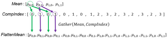
Figure 9.
Illustration of the creation of duplicated mean vectors (Line 23 in Algorithm 4). In this example, the GMM of each set has two Gaussian components, and each mean vector will match with four samples because every set has four input samples. Therefore, the length of the duplicated mean vector array is 16 (the total number of mean vectors multiplied by the sample count in each set).
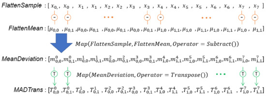
Figure 10.
Illustration of computation of mean deviations and the transpose of mean deviations. is the mean deviation computed from the mean vector of the Gaussian component in the set and the sample.
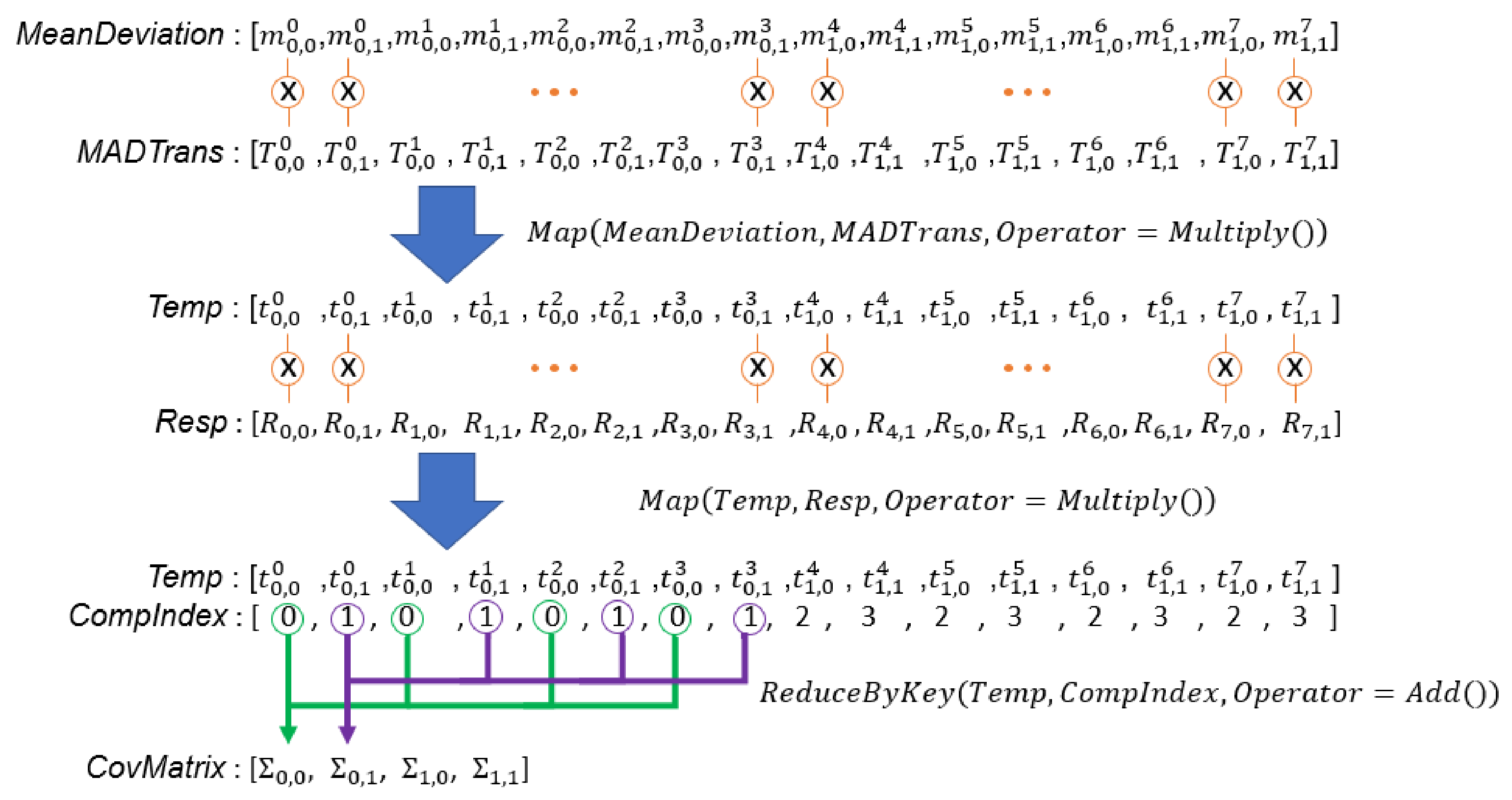
Lines 5, 25, 26, and 28 in Algorithm 3 compute the covariance matrices of all sets using responsibilities, mean deviations, and unnormalized weights. The corresponding code segment in the DPP version algorithm is Lines 25–29 in Algorithm 4. Each mean deviation has to be multiplied with the transpose of itself. Lines 25 and 26 complete this calculation in parallel using MAP primitives. Note that each element in is an n by 1 vector, where n is the number of variables of the input samples. Therefore, the operation at Line 26 is a vector multiplication, and an element in the output array, , is an n by n matrix. The second part of Figure 10 and the first part of Figure 11 illustrate this operation. In addition, the multiplication of responsibility, mean deviation, and the transpose of mean deviation that belong to the same Gaussian component are ultimately accumulated in a matrix. Each matrix is divided by the unnormalized weight of the corresponding Gaussian component to update the covariance matrix of the Gaussian component. This operation is completed in parallel by Lines 28 and 29 in Algorithm 4. Figure 11 illustrates this computation.
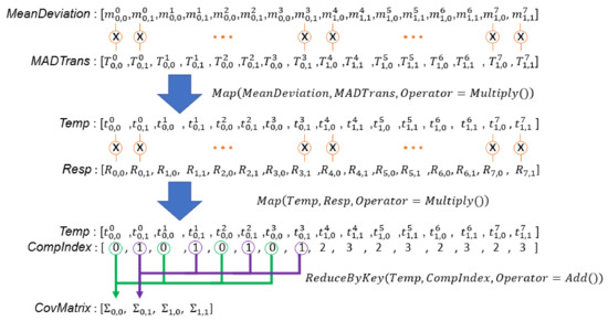
Figure 11.
Illustration of computation of covariance matrices of all sets. is an n by 1 vector, is a 1 by n vector, is an n by n matrix, and is a scalar value.
5.3. E-Step
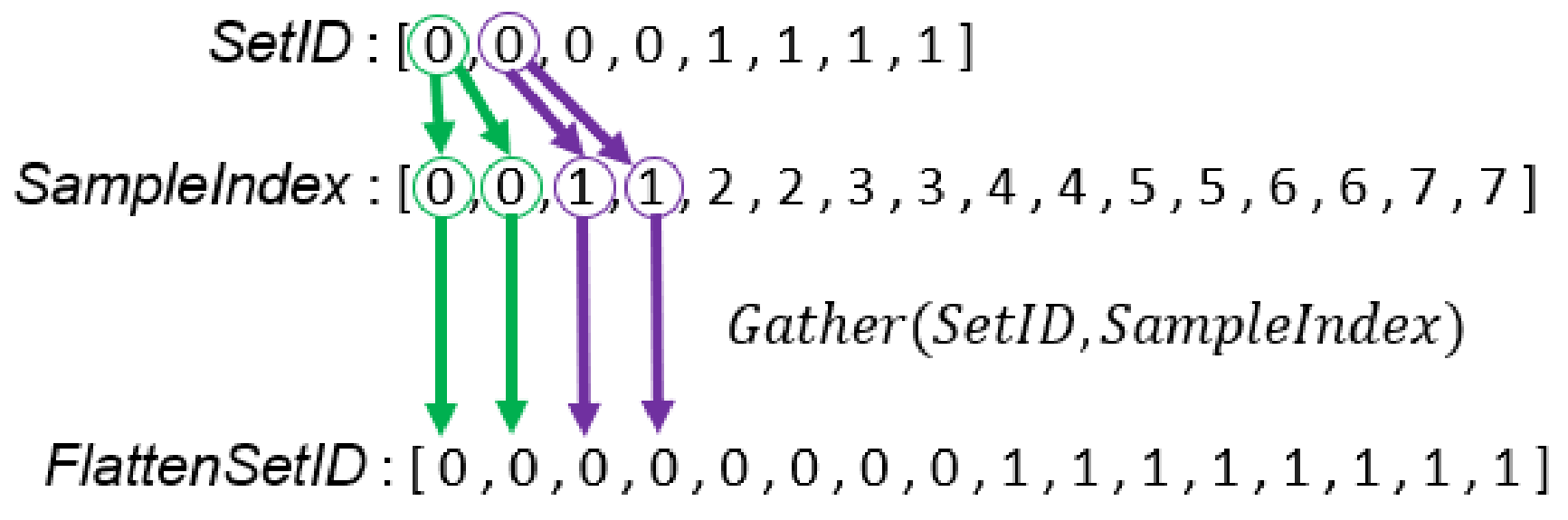
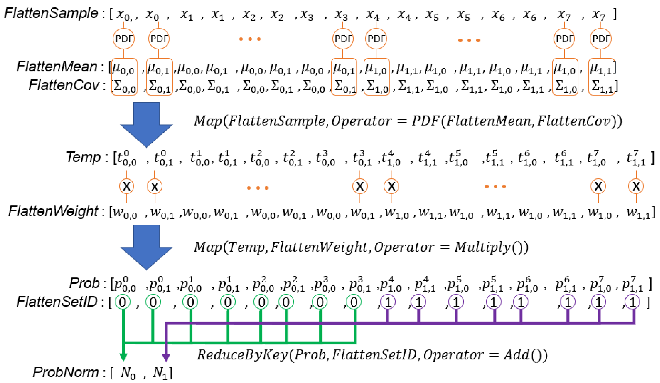
Line 5 and Lines 34–39 in Algorithm 3 estimate the weighted probability densities between all samples and all Gaussian components of the corresponding GMM, and add up all of the weighted probability densities of each set. Therefore, each GMM calculates a . The corresponding code segment in the DPP version algorithm is Lines 31–36 in Algorithm 4. To compute probability densities between all samples and all Gaussian components of the corresponding GMM, we need arrays which store all combinations among input samples, weights, mean vectors, and covariance matrices. These arrays store duplicated samples (), weights (), mean vectors (), and covariance matrices (). We have created and in previous steps. Similar to the procedure for , we create and at Lines 32 and 33 in Algorithm 4. In Line 34, a MAP primitive with the PDF() operator is used to calculate the probability density of any pair between a sample and a Gaussian component. Note that a covariance matrix decomposition is required to compute the probability density of a sample. We directly use an external library to compute the decomposition and do not design the algorithm. To fairly evaluate our algorithm, our evaluation also does not involve this part. Line 35 uses a MAP primitive to compute the weighted probability density using multiple probability density with the corresponding weight. Finally, the probabilities that belongs to the same GMM are added to obtain a value. To complete this task in parallel, we need an array, , with the same length as array. An element in indicates the set ID of the corresponding sample in . As input samples never change, we prepare at Line 11 in Algorithm 4. Figure 12 illustrates the process to create . Line 36 in Algorithm 4 aggregates probabilities that belong to the same GMM to compute array. Figure 13 illustrates the above calculation.
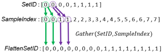
Figure 12.
Illustration of creating the array which stores the corresponding set ID of array.
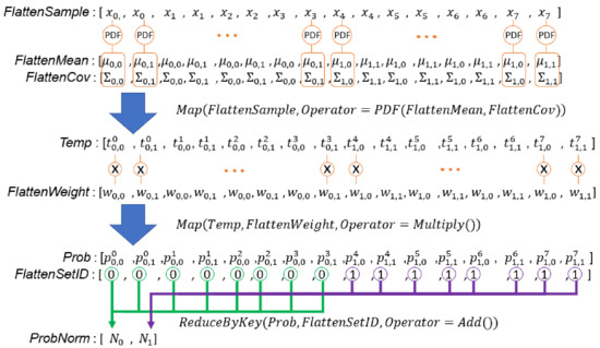
Figure 13.
Illustration of E-step computation by data-parallel primitives. , , and are the weight, mean vector, and covariance matrix of the Gaussian component in the set. is a probability density computed from the sample and the Gaussian component in the set. is of the GMM of set.
5.4. Responsibility Update
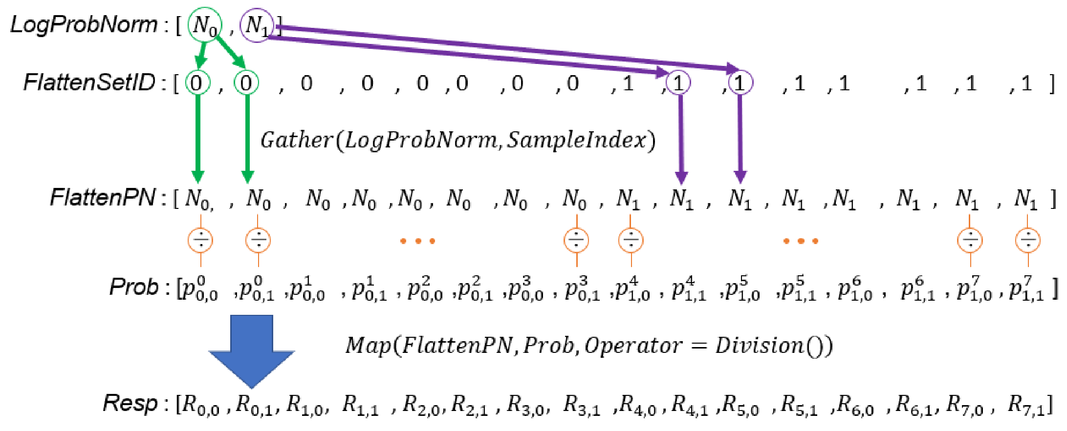
Line 5 and Lines 42–46 in Algorithm 3 divide all weighted probability densities by the of the corresponding set to compute the array. The corresponding code segment in the DPP version algorithm is Line 38 and 39 in Algorithm 4. To complete this task in parallel, we should first prepare an array, , whose length is the same as . Each element in is a value from whose set ID is the same as the corresponding element in . This task is completed by Line 38 in Algorithm 4. Line 39 uses a MAP primitive to calculate the responsibilities by computing element-wise division of and in parallel. Figure 14 illustrates the process of updating responsibilities by data-parallel primitives.
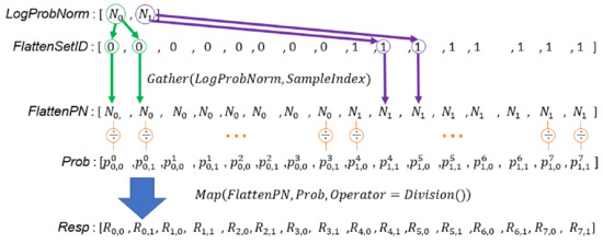
Figure 14.
Illustration of the process of updating responsibilities by data-parallel primitives.
5.5. EM Termination Conditions
When the likelihood value () of each GMM starts to oscillate, it means that the estimation of the GMM has converged to the local optimum, and we can stop the algorithm to save the computational resource. At Lines 41 and 42 in Algorithm 4, we use to compute the absolute difference between each value in before and after updating and use the primitive to calculate the sum of all differences. If the sum is less than a , it means the algorithm has reached stable status. In addition, if the number of iteration reaches the limit set by the user, the EM algorithm should also stop. We simply use the loop at Line 14 in Algorithm 4 to check this termination condition. In any case, as long as the program ends the iteration, the current parameters are the fitting result of the EM algorithm.
5.6. Improvement of the Shared Memory Environment
Algorithm 4 duplicates , , , and to enable parallelization using data-parallel primitives. The algorithm can be used on both distributed memory and shared memory environments because all the arrays processed by data-parallel primitives are equal in length, and can easily be distributed to computing nodes or threads. However, duplicating , , , and needs extra computational time. If we run the algorithm on a shared memory environment, the duplication is not necessary because we can randomly access arrays.
We have to use the MAP primitive with a customizing operator which can access some input arrays randomly. The operator must have the same number of arguments as the MAP primitive, and their arguments have one-to-one correspondence. The arguments in brackets are the array that the operator can randomly access. All elements of the arguments without brackets are computed concurrently. Therefore, the lengths of all arguments without brackets and the output array must be the same. The code segment defines the computation of each element of the arguments without brackets. Line 18 and the operator defined at Line 43 in Algorithm 5 is an example of the MAP primitive with a customizing operator.
Algorithm 5 is the most efficient algorithm for shared memory parallelization. It has the same aim as Algorithm 5; the difference is its use of the MAP primitives with a customizing operator to avoid the array duplication. We remove Line 10 in Algorithm 4. Furthermore, Line 19, Lines 23–24, Lines 32–35, and Lines 38–39 in Algorithm 4 are replaced by the MAP primitives at Line 18, Line 22, Line 30, and Line 34 in Algorithm 5, respectively. In addition, we remove most of the Gather primitives used to duplicate arrays in Algorithm 5.
| Algorithm 5 DPP Version of the Multi-set EM Algorithm for Shared Memory Environment |
|
5.7. Covariance Matrix Computation Simplification
If the number of the variables of input samples is D, the size of the covariance matrix is D by D. We already know the covariance matrix must be a symmetric matrix. Considering the step that the covariance matrix involves, except for the vector multiplication in Line 26 of Algorithm 4, all other operations are scalar operations, so the covariance matrix is still a symmetric matrix, as follows:
where is the covariance matrix of the Gaussian component of the GMM in the set.
Due to the symmetry of the covariance matrix, we can only compute the lower triangular matrix of the covariance matrix to simplify the computation and reduce the memory requirement. From Lines 22–24 in Algorithm 5, we know that a covariance matrix is computed from a mean vector and an input sample. Therefore, each element in a covariance matrix can be computed by Equation (6). With this method, we only access the elements in the lower triangular matrix to complete any computation related to the covariance matrix, to save the computational time and memory. In addition, from Equation (6), we know that the computation of each element in the covariance matrix is independent. We can compute each element in parallel to maximize the parallelization:
where .
Figure 15 is a schematic diagram of the process of computing the covariance matrix when there are three variables of the input samples.
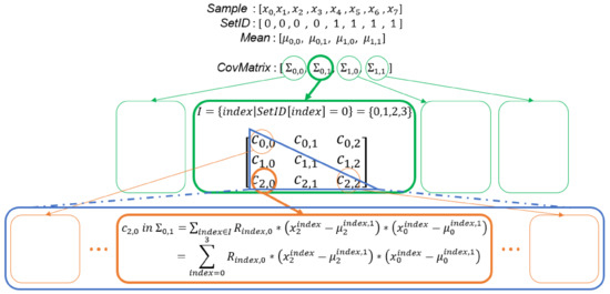
Figure 15.
In this example, two 3-variate GMMs are modeled at the same time, and each GMM has two Gaussian components. The level of parallelism is when the optimization introduced in this section is applied.
6. Experiment
In this section, we evaluate the impact of parameters and the number of threads on the execution time of our proposed algorithms using three different scientific datasets. We conduct the experiments on a supercomputer, Taiwania 2. Each node of Taiwania 2 has two Intel Xeon Gold 6154 18-Cores 3.0GHz and eight NVIDIA® Tesla® V100 SXM2. We implement our proposed algorithms using the VTK-m library [10], a platform that enables scientists to develop scientific data analysis and visualization algorithms using data-parallel primitives. VTK-m supports both CPU and GPU computing backends. When using CPU as the computing backend, VTK-m allows users to use either Intel Threading Building Block (TBB) or OpenMP libraries to run the program using multiple CPU cores. The programs for the performance evaluations of our proposed algorithms which are carried out on CPU are implemented by a VTK-m library that uses Intel TBB.
The three datasets are listed as follows:
- Dataset 1 is hurricane pressure volume data. The resolution is 500 × 500 × 100 and each grid point is a scalar value.
- Dataset 2 is dark matter momentum vector data. The resolution is 64 × 64 × 64 and each grid point is a three-variant vector.
- Dataset 3 is dark matter density ensemble data with 1000 ensemble members. The resolution of each ensemble member is 64 × 64 × 64 and each grid point is a scalar value.
The dataset1 is provided by Scivis Contest 2004 and can be downloaded from its website [39]. Dataset2 and dataset3 are produced by Nyx simulation. The simulation can be downloaded from its official website [40], and we run the simulation by ourselves to generate dataset2 and dataset3. For datasets 1 and 2, we subdivide them into several sub-blocks according to the given block size, and calculate a distribution from samples in each sub-block. As datasets 1 and 2 have different resolutions, we have different block size settings for these two datasets. We subdivide dataset 1 into blocks with block sizes of 8, 16, 32, and 64, and subdivide dataset 2 into block sizes of 2, 4, 8, and 16. For dataset 3, we calculate a distribution from samples across all ensemble members at the same grid points. Therefore, we will compute 64 × 64 × 64 distributions, and each distribution is calculated from 1000 samples.
6.1. Performance Analysis of the Algorithms
Table 1 and Table 2 show the speedup of the proposed histogram and GMM modeling algorithms using a different number of threads on CPU and GPU. We use the execution time for single thread CPU of each dataset as the baseline to calculate the speedup of different settings. When we use two cores, the speedup of both the algorithms and all datasets is almost doubled. When we use 18 cores, the worst speedup of the histogram modeling algorithm is 13.30 times and the worst speedup of the GMM modeling algorithm is 14.74 times. Therefore, both the proposed algorithms have good scalability from using two cores to 18 cores on the CPU. We also test the same algorithms on one NVIDIA® Tesla® V100 SXM2 GPU. As the GPU has a much more extensive computing thread, we gain 48-98x speedup on histogram modeling and 71-460x speedup on GMM modeling for different datasets.

Table 1.
Speedup of our proposed parallel multi-set histogram modeling algorithm.
Table 2.
Speedup of our proposed parallel multi-set GMM modeling algorithm.
6.2. Parameter Analysis of the Algorithms
6.2.1. Histogram
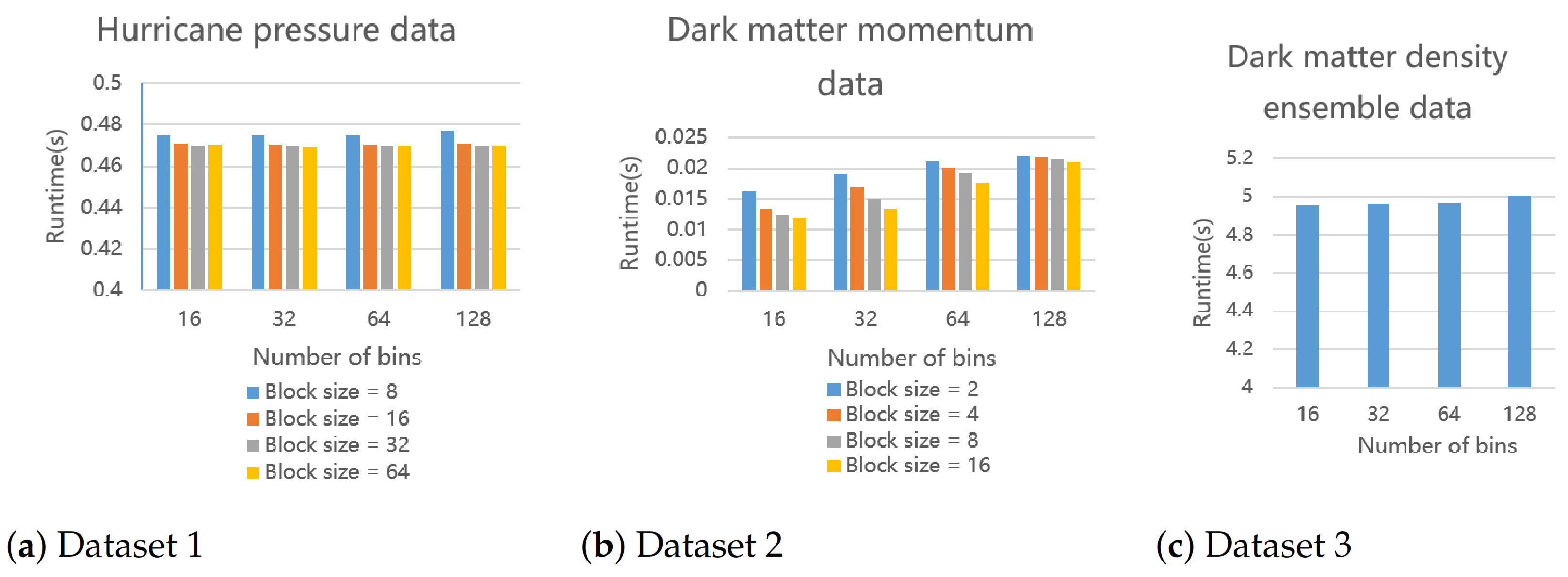
Figure 16 shows the results of the three datasets using 16 3.0 GHz cores to run the parallel histogram modeling algorithm. We can observe that both different block sizes and bin counts have an impact on the execution time. If the block size is smaller or bin count is larger, the execution time will increase. If the block size is smaller (the number of sets increases) or the number of bins is larger, we will have more unique 1D indices (keys) in the array at Line 14 of Algorithm 2. Therefore, more threads are required when the ReduceByKey primitive merges elements with the same key. If the number of samples required to be parallelized is greater than the number of available threads, the execution time will increase.
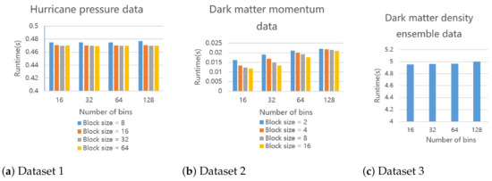
Figure 16.
The execution time of our proposed parallel histogram modeling algorithm. We run it for three datasets on a 16-core CPU under given parameter settings. Dataset 3 is an ensemble data so there is no block size to change.
6.2.2. GMM
In this subsection, we divide the steps of the EM algorithm into five parts to analyze the execution time. They are:
- Time for the E-step.
- Time to update the weights.
- Time to update mean vectors.
- Time to flatten the covariance matrix.
- Time to update the covariance matrix.
Since the number of iterations of the EM algorithm is not fixed, we report the execution time of each step on average for comparison. We can observe the changes in the execution time of these five different steps when the number of Gaussian components and the block size change.
Gaussian component: Figure 17 shows the average execution time of three different datasets with different numbers of Gaussian components. In all datasets, each step requires more execution time when the number of Gaussian components increases. This is because the amount of calculation in each step is positively correlated with the number of Gaussian components in the EM algorithm.
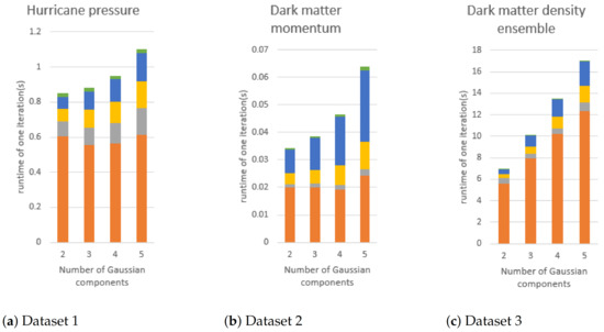
Figure 17.
The execution time of GMM modeling if the number of Gaussian components is changed. The block size of (a,b) is fixed to 16. In the figures, orange, gray, yellow, blue, and green bars are the execution times of E-step, mean vector updating, covariance matrix flattening, and covariance matrix updating, respectively.
Block size: Figure 18 shows the changes in execution time of dataset 1 and dataset 2 when different block sizes are used. We can observe that a smaller block size setting requires a longer execution time in each dataset; this is because a smaller block size setting generates more blocks. Therefore, the total number of sets, S, in Algorithm 5 will increase and the execution time, except for E-step, will increase.
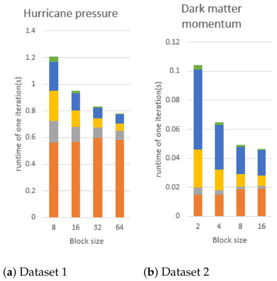
Figure 18.
We fix the number of Gaussian components to 4 and change the block size to conduct this experiment, using dataset1 and dataset2 on the CPU using 16 core. In the figures, orange, gray, yellow, blue, and green bars are the execution time of E-step, mean vector updating, covariance matrix flattening, and covariance matrix updating, respectively. Dataset 3 is an ensemble data so there is no block size to change.
7. Use Cases
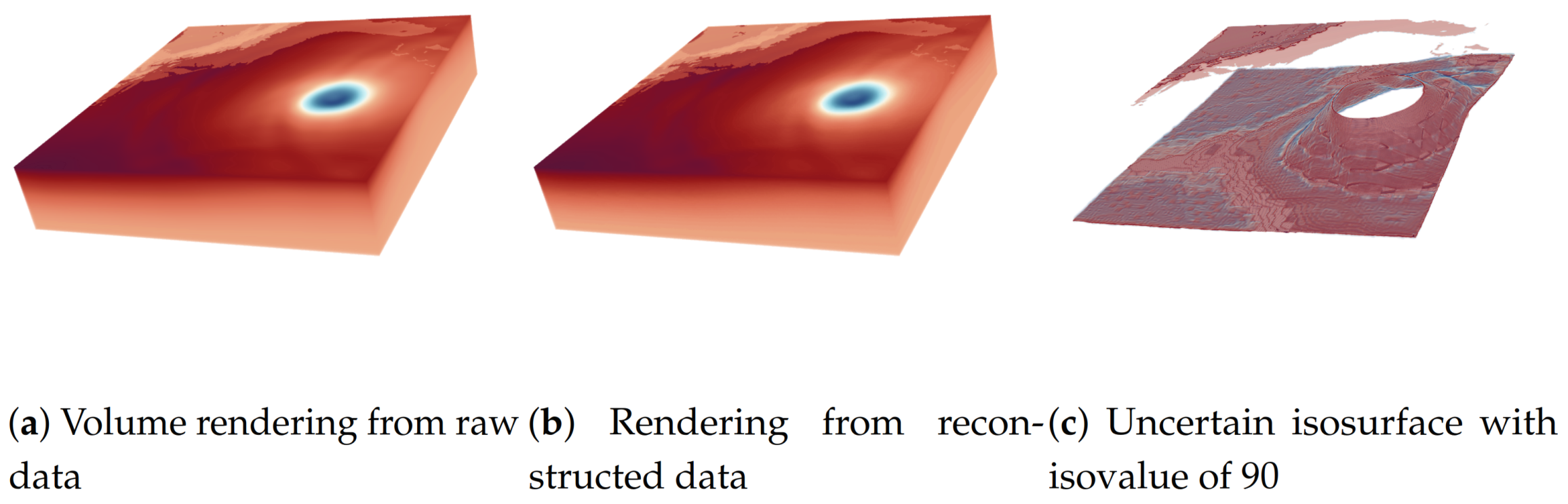
In this use case, we are going to use a more complicated distribution representation to demonstrate our proposed algorithms. Wang et al. [4] proposed a compact distribution-based representation for volume scientific datasets. Their approach subdivides volume data into multiple sub-blocks. The data values in a sub-block are decoupled into value distribution and location information. The value distribution of a sub-block is represented by a histogram. The location information is represented by 3-variant GMMs. If the number of histogram bins is B, the sub-block should store B 3-variant GMMs. Each GMM describes the occurrence probability of data values that belong to a bin in the sub-block space. Each block’s histogram and 3-variant GMMs can be combined using the Bayes rule to compute the value distribution at each grid point and perform arbitrary data analysis and visualization tasks. We use the proposed parallel histogram and GMM modeling algorithms to compute the distribution representation of a hurricane pressure dataset, Isabel. The spatial resolution of Isabel is 500 × 500 × 100, and the size of Isabel is 95 MB. We divide the dataset into sub-blocks, and the size of each sub-block is 16 × 16 × 16. So, Isabel is divided into 32 × 32 × 7 blocks. Each sub-block is modeled by a single-variant histogram with 128 bins. If the frequency of a bin is not 0, we have to compute a 3-variant GMM for the bin. Therefore, we have to compute 7186 histograms and 46226 GMMs in total for the Isabel dataset. We run this use case on NVIDIA® Tesla® V100 SXM2. The time of the histograms and GMMs modeling using the proposed algorithms are 0.165064 seconds and 2.35(0.117 per iteration) seconds, respectively. We also use the Bayes rule described in [4] to compute the value distribution at each grid point and use the data value with the highest probability at each grid point to reconstruct the volume. Figure 19 is the visualization using uncertain isosurface and volume rendering techniques to show the reconstructed dataset. It also validates the correctness of the proposed algorithms using a real scientific dataset.

Figure 19.
The result of using the two proposed parallel multi-set distribution modeling algorithms in a real application.
8. Conclusions and Future Work
This paper presents parallel algorithms of multi-variant histogram and GMM modeling. The algoithms are designed for distribution-based large-scale scientific data processing. The algorithms can efficiently model histograms and GMMs from samples that are divided into multiple sets. We use data-parallel primitives to develop the algorithms because many data-parallel primitives have been used to develop libraries which can execute a code on different hardware architectures, such as multi-core CPU and GPU, without rewriting the code. Therefore, scientists can easily deploy the data processing algorithms on the computing hardware they have. We demonstrate the efficiency of the proposed algorithms and influence of parameters, such as the size of sets, the number of Gaussian components of GMM, the number of bins of histogram, and the number of threads. We also demonstrate the proposed algorithms using two distribution-based scientific data representations. In the future, we would like to extend our work to a parallel library for large-scale scientific data processing and analysis to facilitate the scientists’ research. The library should support more popular data models and file formats of scientific datasets. We should also develop more parallel algorithms for scientific data analysis and visualization from distribution-based representations. The proposed algorithms in this paper will be the core algorithms in the library.
9. Discussion
This section will discuss the pros and cons of the proposed parallel multi-set distribution modeling algorithms. We will compare our proposed algorithm with the serial algorithm and the extension version of the parallel single distribution modeling algorithm. The serial algorithms are simply Algorithm 1 and 3. Several parallel single distribution modeling algorithms are already proposed. A straightforward way to extend them to deal with the multi-set distribution modeling problem is to iterate through every set and use the existing parallel single distribution modeling algorithm to concurrently model samples of each set to a distribution. We call it a parallel single-set distribution modeling algorithm in this subsection. The reported computation time in this section is carried out on a CPU and by the Dataset1 introduced in Section 6.
Table 3 and Table 4 show that the simple serial algorithm is faster than our algorithm when we only use a single core. This is because our algorithm requires extra computation to organize data from all sets for the parallel computation when more cores are available. When only one core is available, our algorithm will spend more time because the total computation load of our algorithm is more than the simple serial algorithm. However, compared with the simple serial algorithm, our algorithm can utilize more computing cores to reduce the total computation time. The computation time of our algorithm is much shorter than the simple serial algorithm when eight cores are available. If more threads are available, our algorithms can further reduce the computation time.
Table 3.
The computation time of our proposed parallel multi-set histogram algorithm and the parallel single-set histogram modeling algorithm. The computation time is in seconds.
Table 4.
The computation time of our proposed parallel multi-set EM algorithm and the parallel single-set histogram modeling algorithm.
We also compare our algorithm with the parallel single-set distribution modeling algorithm. We use OpenMP to implement parallel single-set distribution modeling algorithms and a loop to iterate through all sets. One of the main differences between our proposed and parallel single-set algorithms is the number of parallel procedure calls. The single-set algorithm concurrently processes the data samples that belong to a set to generate one distribution and uses a loop to iterate through all sets. Our proposed algorithm concurrently processes data samples from all sets and generates all distributions. Therefore, the number of the parallel procedure calls of the parallel single-set algorithm is much larger than our proposed algorithm. We know that a parallel procedure not only needs to spend time sharing works to all threads but also has to synchronize all threads at the end of the parallel procedure to ensure the program can leave the parallel procedure and continue. The work sharing and thread synchronization are the overhead of a parallel procedure. Although the overhead is usually very short, it will count up to a large amount if the program calls the parallel procedure many times.
The columns with block size 8 in Table 3 and Table 4 show that our algorithm has a much better speedup than the parallel single-set algorithm. In this experiment, the dataset is subdivided into around 50 thousand sets if the block size is 8. Therefore, the parallel single-set algorithms have to pay overhead to handle the work sharing and the thread synchronization and not gain a good speedup. In addition, if more cores are used, the overhead is essentially longer because more threads are required to synchronize. Therefore, it does not guarantee that the total computation time is shorter if more cores are used. The single-set GMM modeling has a negative speedup because it uses much more parallel primitives than the histogram modeling. We also carry out the same experiment but change the block size to 2. In this experiment, the dataset is subdivided into around three million sets. The number of sets of the block size of 2 is much more than that of 8. In Table 3 and Table 4, we can observe that the computation time of the single-set algorithms becomes much longer because it has to handle much more overhead. By contrast, the computation time of our proposed algorithms stays on the same scale.
Author Contributions
Conceptualization, K.-C.W.; Project administration, K.-C.W.; Resources, K.-C.W.; Software, H.-Y.Y., Z.-R.L. and K.-C.W.; Supervision, K.-C.W.; Writing—original draft, H.-Y.Y., Z.-R.L. and K.-C.W.; Writing—review & editing, K.-C.W. All authors have read and agreed to the published version of the manuscript.
Funding
This research was funded by “Ministry of Science and Technology, Taiwan” grant number “109B0054”.
Institutional Review Board Statement
Not applicable.
Informed Consent Statement
Not applicable.
Data Availability Statement
Not applicable.
Conflicts of Interest
The authors declare no conflict of interest.
References
- Dutta, S.; Chen, C.M.; Heinlein, G.; Shen, H.W.; Chen, J.P. In situ distribution guided analysis and visualization of transonic jet engine simulations. IEEE Trans. Vis. Comput. Graph. 2016, 23, 811–820. [Google Scholar] [CrossRef] [PubMed]
- Dutta, S.; Shen, H.W.; Chen, J.P. In Situ prediction driven feature analysis in jet engine simulations. In Proceedings of the 2018 IEEE Pacific Visualization Symposium (PacificVis), Kobe, Japan, 10–13 April 2018; pp. 66–75. [Google Scholar]
- Thompson, D.; Levine, J.A.; Bennett, J.C.; Bremer, P.T.; Gyulassy, A.; Pascucci, V.; Pébay, P.P. Analysis of large-scale scalar data using hixels. In Proceedings of the 2011 IEEE Symposium on Large Data Analysis and Visualization, Providence, RI, USA, 23–24 October 2011; pp. 23–30. [Google Scholar]
- Wang, K.C.; Lu, K.; Wei, T.H.; Shareef, N.; Shen, H.W. Statistical visualization and analysis of large data using a value-based spatial distribution. In Proceedings of the 2017 IEEE Pacific Visualization Symposium (PacificVis), Seoul, Korea, 18–21 April 2017; pp. 161–170. [Google Scholar]
- Kumar, N.P.; Satoor, S.; Buck, I. Fast parallel expectation maximization for gaussian mixture models on gpus using cuda. In Proceedings of the 2009 11th IEEE International Conference on High Performance Computing and Communications, Seoul, Korea, 25–27 June 2009; pp. 103–109. [Google Scholar]
- Kwedlo, W. A parallel EM algorithm for Gaussian mixture models implemented on a NUMA system using OpenMP. In Proceedings of the 2014 22nd Euromicro International Conference on Parallel, Distributed, and Network-Based Processing, Seoul, Korea, 25–27 June 2014; pp. 292–298. [Google Scholar]
- Shams, R.; Kennedy, R. Efficient histogram algorithms for NVIDIA CUDA compatible devices. In Proceedings of the ICSPCS 2007, Dubai, United Arab Emirates, 24–27 November 2007; pp. 418–422. [Google Scholar]
- Li, G.; Xu, J.; Zhang, T.; Shan, G.; Shen, H.W.; Wang, K.C.; Liao, S.; Lu, Z. Distribution-based particle data reduction for in-situ analysis and visualization of large-scale n-body cosmological simulations. In Proceedings of the 2020 IEEE Pacific Visualization Symposium (PacificVis), Tianjin, China, 3–5 June 2020; pp. 171–180. [Google Scholar]
- Bell, N.; Hoberock, J. Thrust: A productivity-oriented library for CUDA. In GPU Computing Gems Jade Edition; Elsevier: Amsterdam, The Netherlands, 2012; pp. 359–371. [Google Scholar]
- Moreland, K.; Sewell, C.; Usher, W.; Lo, L.t.; Meredith, J.; Pugmire, D.; Kress, J.; Schroots, H.; Ma, K.L.; Childs, H.; et al. Vtk-m: Accelerating the visualization toolkit for massively threaded architectures. IEEE Comput. Graph. Appl. 2016, 36, 48–58. [Google Scholar] [CrossRef] [PubMed]
- Sewell, C.M. Piston: A Portable Cross-Platform Framework for Data-Parallel Visualization Operators; Technical Report; Los Alamos National Lab. (LANL): Los Alamos, NM, USA, 2012. [Google Scholar]
- Lee, T.Y.; Shen, H.W. Efficient local statistical analysis via integral histograms with discrete wavelet transform. IEEE Trans. Vis. Comput. Graph. 2013, 19, 2693–2702. [Google Scholar] [PubMed]
- Wei, T.H.; Dutta, S.; Shen, H.W. Information guided data sampling and recovery using bitmap indexing. In Proceedings of the 2018 IEEE Pacific Visualization Symposium (PacificVis), Kobe, Japan, 10–13 April 2018; pp. 56–65. [Google Scholar]
- Wei, T.H.; Chen, C.M.; Woodring, J.; Zhang, H.; Shen, H.W. Efficient distribution-based feature search in multi-field datasets. In Proceedings of the 2017 IEEE Pacific Visualization Symposium (PacificVis), Seoul, Korea, 18–21 April 2017; pp. 121–130. [Google Scholar]
- Wang, K.C.; Wei, T.H.; Shareef, N.; Shen, H.W. Ray-based exploration of large time-varying volume data using per-ray proxy distributions. IEEE Trans. Vis. Comput. Graph. 2019, 26, 3299–3313. [Google Scholar] [CrossRef] [PubMed]
- Liu, S.; Levine, J.A.; Bremer, P.T.; Pascucci, V. Gaussian mixture model based volume visualization. In Proceedings of the IEEE Symposium on Large Data Analysis and Visualization (LDAV), Seattle, WA, USA, 14–15 October 2012; pp. 73–77. [Google Scholar]
- Li, C.; Shen, H.W. Winding angle assisted particle tracing in distribution-based vector field. In Proceedings of the SIGGRAPH Asia 2017 Symposium on Visualization, Bangkok, Thailand, 27–30 November 2017; pp. 1–8. [Google Scholar]
- Dutta, S.; Shen, H.W. Distribution driven extraction and tracking of features for time-varying data analysis. IEEE Trans. Vis. Comput. Graph. 2015, 22, 837–846. [Google Scholar] [CrossRef] [PubMed]
- Wang, K.C.; Xu, J.; Woodring, J.; Shen, H.W. Statistical super resolution for data analysis and visualization of large scale cosmological simulations. In Proceedings of the 2019 IEEE Pacific Visualization Symposium (PacificVis), Bangkok, Thailand, 23–26 April 2019; pp. 303–312. [Google Scholar]
- Chaudhuri, A.; Lee, T.Y.; Shen, H.W.; Peterka, T. Efficient range distribution query in large-scale scientific data. In Proceedings of the 2013 IEEE Symposium on Large-Scale Data Analysis and Visualization (LDAV), Atlanta, GA, USA, 13–14 October 2013; pp. 125–126. [Google Scholar]
- Chaudhuri, A.; Wei, T.H.; Lee, T.Y.; Shen, H.W.; Peterka, T. Efficient range distribution query for visualizing scientific data. In Proceedings of the 2014 IEEE Pacific Visualization Symposium, Yokohama, Japan, 4–7 March 2014; pp. 201–208. [Google Scholar]
- Chen, C.M.; Biswas, A.; Shen, H.W. Uncertainty modeling and error reduction for pathline computation in time-varying flow fields. In Proceedings of the 2015 IEEE Pacific Visualization Symposium (PacificVis), Hangzhou, China, 14–17 April 2015; pp. 215–222. [Google Scholar]
- Blelloch, G.E. Vector Models for Data-Parallel Computing; MIT Press: Cambridge, MA, USA, 1990; Volume 2. [Google Scholar]
- Lessley, B.; Perciano, T.; Heinemann, C.; Camp, D.; Childs, H.; Bethel, E.W. DPP-PMRF: Rethinking optimization for a probabilistic graphical model using data-parallel primitives. In Proceedings of the 2018 IEEE 8th Symposium on Large Data Analysis and Visualization (LDAV), Berlin, Germany, 21–21 October 2018; pp. 34–44. [Google Scholar]
- Austin, W.; Ballard, G.; Kolda, T.G. Parallel tensor compression for large-scale scientific data. In Proceedings of the 2016 IEEE international parallel and distributed processing symposium (IPDPS), Chicago, IL, USA, 23–27 May 2016; pp. 912–922. [Google Scholar]
- Hawick, K.A.; Coddington, P.D.; James, H.A. Distributed frameworks and parallel algorithms for processing large-scale geographic data. Parallel Comput. 2003, 29, 1297–1333. [Google Scholar] [CrossRef]
- Yenpure, A.; Childs, H.; Moreland, K.D. Efficient Point Merging Using Data Parallel Techniques; Technical Report; Sandia National Lab. (SNL-NM): Albuquerque, NM, USA, 2019. [Google Scholar]
- Larsen, M.; Labasan, S.; Navrátil, P.A.; Meredith, J.S.; Childs, H. Volume Rendering Via Data-Parallel Primitives. In Proceedings of the 15th Eurographics Symposium on Parallel Graphics and Visualization, Cagliari, Sardinia, Italy, 25–26 May 2015; pp. 53–62. [Google Scholar]
- Lessley, B.; Li, S.; Childs, H. HashFight: A Platform-Portable Hash Table for Multi-Core and Many-Core Architectures. Electron. Imaging 2020, 2020, 376-1–376-13. [Google Scholar] [CrossRef]
- Li, S.; Marsaglia, N.; Chen, V.; Sewell, C.M.; Clyne, J.P.; Childs, H. Achieving Portable Performance for Wavelet Compression Using Data Parallel Primitives. In Proceedings of the 17th Eurographics Symposium on Parallel Graphics and Visualization, Barcelona, Spain, 12–13 June 2017; pp. 73–81. [Google Scholar]
- Lessley, B.; Perciano, T.; Mathai, M.; Childs, H.; Bethel, E.W. Maximal clique enumeration with data-parallel primitives. In Proceedings of the IEEE 7th Symposium on Large Data Analysis and Visualization (LDAV), Phoenix, AZ, USA, 2 October 2017; pp. 16–25. [Google Scholar]
- Esbensen, K.H.; Guyot, D.; Westad, F.; Houmoller, L.P. Multivariate Data Analysis: In Practice: An Introduction to Multivariate Data Analysis and Experimental Design. Available online: https://www.google.com/books?hl=en&lr=&id=Qsn6yjRXOaMC&oi=fnd&pg=PA1&dq=Multivariate+data+analysis:+in+practice:+an+introduction+to+++multivariate+data+analysis+and+experimental+design&ots=cD1l2TqOT2&sig=1CUTO79G3V3-gGuEODBYBODjDJs (accessed on 26 September 2021).
- Zhang, Y. Improving the accuracy of direct histogram specification. Electron. Lett. 1992, 28, 213–214. [Google Scholar] [CrossRef]
- Jones, M.; Viola, P. Fast Multi-View Face Detection. Available online: https://www.researchgate.net/profile/Michael-Jones-66/publication/228362107_Fast_multi-view_face_detection/links/0fcfd50d35f8570d70000000/Fast-multi-view-face-detection.pdf (accessed on 26 September 2021).
- Chakravarti, R.; Meng, X. A study of color histogram based image retrieval. In Proceedings of the Sixth International Conference on Information Technology: New Generations, Las Vegas, NV, USA, 27–29 April 2009; pp. 1323–1328. [Google Scholar]
- Bachtis, D.; Aarts, G.; Lucini, B. Extending machine learning classification capabilities with histogram reweighting. Phys. Rev. E 2020, 102, 033303. [Google Scholar] [CrossRef] [PubMed]
- Hazarika, S.; Biswas, A.; Shen, H.W. Uncertainty visualization using copula-based analysis in mixed distribution models. IEEE Trans. Visual Comput. Graphics 2017, 24, 934–943. [Google Scholar] [CrossRef] [PubMed]
- Hazarika, S.; Dutta, S.; Shen, H.W.; Chen, J.P. Codda: A flexible copula-based distribution driven analysis framework for large-scale multivariate data. IEEE Trans. Visual Comput. Graphics 2018, 25, 1214–1224. [Google Scholar] [CrossRef] [PubMed]
- IEEE Visualization 2004 Contest. Available online: http://vis.computer.org/vis2004contest/ (accessed on 26 September 2021).
- Nyx Simulation. Available online: https://amrex-astro.github.io/Nyx/ (accessed on 26 September 2021).


Publisher’s Note: MDPI stays neutral with regard to jurisdictional claims in published maps and institutional affiliations. |
© 2021 by the authors. Licensee MDPI, Basel, Switzerland. This article is an open access article distributed under the terms and conditions of the Creative Commons Attribution (CC BY) license (https://creativecommons.org/licenses/by/4.0/).