An Algorithm for Making Regime-Changing Markov Decisions

Abstract

In industrial applications, the processes of optimal sequential decision making are naturally formulated and optimized within a standard setting of Markov decision theory. In practice, however, decisions must be made under incomplete and uncertain information about parameters and transition probabilities. This situation occurs when a system may suffer a regime switch changing not only the transition probabilities but also the control costs. After such an event, the effect of the actions may turn to the opposite, meaning that all strategies must be revised. Due to practical importance of this problem, a variety of methods has been suggested, ranging from incorporating regime switches into Markov dynamics to numerous concepts addressing model uncertainty. In this work, we suggest a pragmatic and practical approach using a natural re-formulation of this problem as a so-called convex switching system, we make efficient numerical algorithms applicable.

1. Introduction

Decision-theoretic planning is naturally formulated and solved using Markov Decision Processes (MDPs, see [1]). This theory provides a fundamental and intuitive formalism not only for sequential decision optimization, but also for diverse learning problems in stochastic domains. A typical goal in such framework is to model an environment as a set of states and actions that can be performed to control these states. Thereby, the goal is to drive the system maximizing specific performance criteria.

The methodologies of MDPs have been successfully applied to (stochastic) planning, learning, robot control, and game playing problems. In fact, MDPs nowadays provide a standard toolbox for learning techniques in sequential decision making. To explain our contribution to this traditional and widespread area, let us consider a simplified example of motion control. Suppose that a robot is moving in two horizontal directions on a rectangular grid whose cells are identified with the states of the system. At any time step, there are four actions to guide the robot from the current position to one of the neighboring cells. These actions are UP, DOWN, RIGHT, LEFT, which command a move to the corresponding direction. However, the success of these actions is uncertain and is state-dependent: For instance, a command (UP) may not always cause a transition to the intended (upper) cell, particularly if the robot is at the (upper) boundary. The controller aims to reach a pre-specified target cell at minimal total costs. These costs are accumulated each time when a control is applied and depend on the current position—the cell currently occupied—accounting for obstacles and other adverse circumstances that may be encountered at some locations. In mathematical terms, such a motion is determined by a so-called controlled discrete-time discrete-space Markov chain. In a more realistic situation, the environment is dynamic: The target can suddenly change its location, or navigation through certain cells can become more difficult, changing the control costs and transitions. In principle, such problems can be addressed in terms of the so-called partially observable Markov decision processes (POMDPs, see [2]), but this approach may turn out to be cumbersome due its higher complexity than that of ordinary MDPs. Instead, we suggest a technique which overcomes this difficulty by a natural and direct modeling in terms of a finite number of Markov decision processes (sharing the same set of sets and actions), each active in a specific regime, when the regime changes, another Markov decision processes takes over. Thereby, the regime is not directly observable, thus the controller must guess which of those Markov decision processes is valid at the current decision time: Determining an optimal control becomes challenging due to regime switches. Surprisingly, one can re-formulate such control problems as a convex switching system [3], in order to take advantage from efficient numerical schemes and advanced error control. As a result, we obtain sound algorithms for solutions of regime-modulated Markov decision problems.

This work models random environment as selection of a finite-number ordinary Markov Decision Processes which are mixed by uncertain observations. On this account, we follow a traditional path facing well-known difficulties originated from high-dimensional state spaces and all problems from incorporating an information flow into a centralized decision process. However, let us emphasize that there is an approach which aims to bypass some of the problems through an alternative modeling. Namely, a game-theoretic framework has attracted significant attention (see [4,5]) as an alternative to the traditional centralized decision optimization within a random and dynamic environment. Here, individual agents aiming at selfishly maximizing their own wealth are acting in a game whose equilibrium replaces a centralized decision optimization. In such a context, the process of gathering and utilizing information is easier to model and manage since the individual strategy optimization is simpler and more efficient in collecting and processing all relevant information which may be private, noisy and highly dispersed.

Before we turn to technical details, let us we summarize in the notations and abbreviations used in this work

Table 1. Notations and measurement units.

stochastic kernel	${\mathcal{K}}_t^a$	vector with unit entries	$\overrightarrow{1}$	volume	cubic meter
controlled probability	${\mathbb{P}}^{x,\pi }$	$l^1$-norm	$\parallel ·\parallel$	area	hectare
controlled expectation	${\mathbb{E}}^{x,\pi }$	maximum	⋁	currency	USD
Bellman operator	${\mathcal{T}}_t$	binding by row	⊔	costs	USD per hectare

.

2. Discrete-Time Stochastic Control

First, let us review a finite-horizon control theory. Consider a random dynamics within a time horizon $\{0,1,\dots ,T\}\subset \mathbb{N}$ whose state x evolves in a state space $\mathcal{X}$ (subset of a Euclidean space) and is controlled by actions a from a finite action set A. The mapping ${\pi }_t:\mathcal{X}\mapsto A$, describing the action ${\pi }_t\left(x\right)$ that the controller takes at time $t=0,\dots T$ in the situation $x\in \mathcal{X}$ is referred to as decision rule. A sequence of decision rules $\pi ={\left({\pi }_t\right)}_{t=0}^{T-1}$ is called a policy. Given a family of

$$\mathrm{stochastic}\mathrm{kernels}{\mathcal{K}}_t^a(x,d{x}^{\prime }),t=0,\dots ,T-1a\in A\mathrm{on}\mathcal{X},$$

there exists an appropriately constructed probability space which supports a stochastic process ${\left(X_t\right)}_{t=0}^T$ such that for each initial point $x_0\in \mathcal{X}$ and each policy $\pi ={\left({\pi }_t\right)}_{t=0}^{T-1}$ there exists a measure ${\mathbb{P}}^{x_0,\pi }$ and such that

$${\mathbb{P}}^{x_0,\pi }(X_0=x_0)=1,{\mathbb{P}}^{x_0,\pi }(X_{t+1}\in B|X_0,\dots ,X_t)={\mathcal{K}}_t^{{\pi }_t\left(X_t\right)}(X_t,B)$$

(1)

holds for $t=0,\dots ,T-1$ for each measurable $B\subset \mathcal{X}$. Such a system is called controlled Markovian evolution. The interpretation is that if at time t the process state is $X_t$ and the action ${\pi }_t\left(X_t\right)$ is applied, then the distribution $K_t^{{\pi }_t\left(X_t\right)}(X_t,·)$ randomly changes the state from $X_t$ to $X_{t+1}$.

Stochastic kernels are equivalently described in terms of transition operators. The transition operator, associated with the stochastic kernel ${\mathcal{K}}_t^a$ will be denoted by the same letter, but it acts on functions $v:\mathcal{X}\to \mathbb{R}$ by

$$({\mathcal{K}}_t^{a}vs.)\left(x\right)={\int }_{\mathcal{X}}v\left(x^{\prime }\right){\mathcal{K}}_t^a(x,d{x}^{\prime })x\in \mathcal{X},t=0,\dots ,T-1$$

(2)

whenever the above integrals are well-defined.

Having introduced such controlled Markovian dynamics, let us turn to control costs now. Suppose that for each time $t=0,\dots ,T-1$, we are given the t-step reward function $r_t:\mathcal{X}\times A\mapsto \mathbb{R}$ where $r_t(x,a)$ represents the reward for applying an action $a\in A$ when the state of the system is $x\in \mathcal{X}$ at time t. At the end of the time horizon, at time T, it is assumed that no action can be taken. Here, if the system is in a state x, a scrap value $r_T\left(x\right)$, described by a pre-specified scrap function $r_T:\mathcal{X}\to \mathbb{R}$ is collected. The expectation of the cumulative reward from following a policy $\pi$ is referred to as policy value:

$$v_0^{\pi }\left(x\right)={\mathbb{E}}^{x,\pi }\left(\sum _{t=0}^{T-1}{r}_t(X_t,{\pi }_t\left(X_t\right))+r_T\left(X_T\right)\right),x\in \mathcal{X},$$

where ${\mathbb{E}}^{x,\pi }$ denotes the expectation over the controlled Markov chain whose distribution is defined by (1). For $t=0,\dots ,T-1$, introduce the backward induction operator

$$\begin{array}{c}\hfill {\mathcal{T}}_t^{a}v\left(x\right)=r_t(x,a)+{\mathcal{K}}_t^{a}v\left(x\right),x\in \mathcal{X},a\in A\end{array}$$

(3)

which acts on each measurable function $v:\mathcal{X}\to \mathbb{R}$ where ${\mathcal{K}}_t^{a}v$ is well-defined. The policy value is obtained as a result of the recursive procedure

$$\begin{array}{c}\hfill v_T^{\pi }=r_T,v_t^{\pi }\left(x\right)={\mathcal{T}}_t^{\pi \left(x\right)}{v}_{t+1}^{\pi }\left(x\right)x\in \mathcal{X},\mathrm{for}t=T-1,\dots ,0\end{array}$$

(4)

which is referred to as the policy iteration. The value of a “best possible” policy is addressed using

$$v_0^{*}\left(x\right)=\underset{\pi }{sup}{v}_0^{\pi }\left(x\right),x\in \mathcal{X},$$

(5)

where $\pi$ runs through the set of all policies, the function $v_0^{*}$ is called the value function. The goal of the optimal control is to find a policy ${\pi }^{*}={\left({\pi }_t^{*}\right)}_{t=0}^{T-1}$ where the above maximization is attained:

$$v_0^{{\pi }^{*}}\left(x\right)=v_0^{*}\left(x\right)\mathrm{for}\mathrm{each}x\in \mathcal{X}.$$

Such policy optimization is well-defined (see [6], p. 199). Thereby, the calculation of an optimal policy ${\pi }^{*}$ is performed in the following framework: For $t=0,\dots ,T-1$, introduce the Bellman operator

$$\begin{array}{c}\hfill {\mathcal{T}}_{t}v\left(x\right)=\underset{a\in A}{max}\left(r_t(x,a)+{\mathcal{K}}_t^{a}v\left(x\right)\right),x\in \mathcal{X}\end{array}$$

(6)

which acts on each measurable function $v:\mathcal{X}\to \mathbb{R}$ where ${\mathcal{K}}_t^{a}v$ is well-defined for all $a\in A$. Further, consider the Bellman recursion, (also called backward induction)

$$\begin{array}{c}\hfill v_T^{*}=r_T,v_t^{*}={\mathcal{T}}_t{v}_{t+1}^{*}\mathrm{for}t=T-1,\dots ,0.\end{array}$$

(7)

There solution ${\left(v_t^{*}\right)}_{t=0}^T$ to the above Bellman recursion returns the value function $v_0^{*}$ and determines an optimal policy ${\pi }^{*}$ via

$${\pi }_t^{*}\left(x\right)={\mathrm{argmax}}_{a\in A}\left(r_t(x,a)+{\mathcal{K}}_t^a{v}_{t+1}^{*}\left(x\right)\right),x\in \mathcal{X},t=0,\dots ,T-1.$$

(8)

Remark 1.

In practice, discounted versions the above stochastic control are popular. These are obtained by replacing the stochastic kernel ${\mathcal{K}}_t^a$ by $\kappa {\mathcal{K}}_t^a$ in the backward induction where $\kappa \in [0,1]$ is a discount factor. The advantage of this approach is that for long time horizons, the optimal policy becomes stationary, provided that all rewards and transition kernels are time-independent.

3. Markov Decisions under Partial Observation

In view of the general framework from Section 2, the classical Markov Decision Processes (MDPs) are obtained by specifying controlled Markovian evolution ${\left(X_t\right)}_{t=0}^T$ in terms of assumptions on the state space and on the transition kernels. Here, the state space is given by a finite set P such that states are driven in terms of

$$\mathrm{stochastic}\mathrm{matrices}{({\alpha }_{p,p^{\prime }}^a)}_{p,p^{\prime }\in P},a\in A.$$

(9)

indexed by a finite number of actions $a\in A$ with the interpretation that ${\alpha }_{p,p^{\prime }}^a\in [0,1]$ stands for the transition probability from $p\in P$ to $p^{\prime }\in P$ if the action $a\in A$ was taken. In this settings, the stochastic kernels ${\mathcal{K}}_t^a$ are acting functions $v:P\to \mathbb{R}$ by

$${\mathcal{K}}_t^{a}v\left(p\right)=\sum _{p^{\prime }\in P}{\alpha }_{p,p^{\prime }}^{a}v\left(p^{\prime }\right)p\in P,t=0,\dots T-1.$$

(10)

There is no specific assumption on scrap and reward functions, they are given by following mappings on the state space P:

$$p\to r_T\left(p\right),(p,a)\mapsto r_t(p,a),t=0,\dots ,T-1,a\in A.$$

(11)

In this work, we consider control problems where a finite number of Markov decision problems are involved, sharing the same state space: each is activated by a certain regime. For this reason, we introduce a selection of MDPs indexed by a finite set S of regimes. Here, we assume that stochastic matrices as in (9) and control costs as in (11) are now indexed by S:

$$\begin{array}{c}{({\alpha }_{p,p^{\prime }}^a\left(s\right))}_{p,p^{\prime }\in P},p\to r_T\left(p\right)\left(s\right),\\ (p,a)\mapsto r_t(p,a)\left(s\right),t=0,\dots ,T-1,\end{array}a\in A,s\in S.$$

(12)

Let us now consider decision making under incomplete information. Given family of Markov decision problems as in (12), the controller deals with a dynamic mixture of these problems in the sense that each of these MDPs becomes valid under a certain regime which changes exogenously in an uncontrolled way and is not observed directly. More precisely, interpreting each probability distribution $\widehat{s}={\left(\widehat{s}\left(s\right)\right)}_{s\in S}$ on S as controllers believe about the current regime, we introduce the following convex mixtures of the ingredients (12):

$$\begin{array}{c}{\alpha }_{p,p^{\prime }}^a\left(\widehat{s}\right)={(\sum _{s\in S}\widehat{s}\left(s\right){\alpha }_{p,p^{\prime }}^a\left(s\right))}_{p,p^{\prime }\in P}p\to \sum _{s\in S}\widehat{s}\left(s\right)r_T\left(p\right)\left(s\right),\\ (p,a)\mapsto \sum _{s\in S}\widehat{s}\left(s\right)r_t(p,a)\left(s\right),t=0,\dots ,T-1,\end{array}a\in A,\widehat{s}\in \widehat{S}.$$

(13)

where $\widehat{S}$ stands for the simplex of all probability distributions on S. That is, the transition kernels and the control costs are now modulated by an external variable $\widehat{s}\in \widehat{S}$ which represents the evolution of controller’s believe about the current situation. To describe its dynamics, we suppose that the information is updated dynamically through the observation of another process ${\left(y_t\right)}_{t=1}^T$ which follows the so-called hidden Markov dynamics. Let us introduce this concept before we finish the definition of our regime-changing Markov decision problem.

Consider a time-homogeneous Markov chain ${\left(s_t\right)}_{t=0}^T$ evolving on a

$$\begin{array}{c}\mathrm{finite}\mathrm{space}S\mathrm{which}\mathrm{is}\mathrm{identified}\mathrm{with}\mathrm{the}\mathrm{set}\mathrm{of}\mathrm{orthonormal}\mathrm{basis}\\ \mathrm{vectors}\mathrm{of}\mathrm{a}\mathrm{finite}-\mathrm{dimensional}\mathrm{Euclidean}\mathrm{space}.\end{array}$$

(14)

Assume that this Markov chain is governed by the stochastic matrix $\Gamma ={\left({\Gamma }_{s,s^{\prime }}\right)}_{s,s^{\prime }\in S}$. It is supposed that the evolution of ${\left(s_t\right)}_{t=0}^T$ is unobservable, representing a hidden regime. The available information is realized by another stochastic process ${\left(y_t\right)}_{t=0}^T$ taking values in a space Y, such that at any time t, the distribution of the next observation $y_{t+1}$ depends on the past $\{y_0,\dots ,y_t\}$ through the recent state $s_t$ only. More precisely, we suppose that ${\left((s_t,y_t)\right)}_{t=0}^T$ follows a Markov process whose transition operators are acting on functions $v:S\times Y\to \mathbb{R}$ as

$$(s,y)\mapsto \sum _{s^{\prime }\in S}{\int }_{Y}v(s^{\prime },y^{\prime }){\Gamma }_{s,s^{\prime }}{\mu }_s\left(\mathrm{d}{y}^{\prime }\right).$$

(15)

Here, ${\left({\mu }_s\right)}_{s\in \mathcal{S}}$ stands for the family of distributions for the next-time observation of $y_{t+1}$, conditioned on $s_t=s\in S$. For each $s\in S$, we assume that the distribution ${\mu }_s$ is absolutely continuous with respect to a reference measure $\mu$ on Y and introduce the densities

$${\nu }_s\left(y\right)=\frac{\mathrm{d}{\mu }_s}{\mathrm{d}\mu }\left(y\right)\mathrm{for}y\in Y\mathrm{and}s\in S.$$

Since the state evolution ${\left(s_t\right)}_{t=0}^T$ is not available, one must rely on the believe distribution ${\widehat{s}}_t$ of the state $s_t$, conditioned on the observations $y_0,\dots ,y_t$. With this, the hidden state estimates ${\left({\widehat{s}}_t\right)}_{t=0}^T$ yield a process that takes values in the set $\widehat{S}$ of all probability measures on S which is identified with the convex hull of S due to (14). It turns out that although the observation process ${\left(y_t\right)}_{t=0}^T$ is non-Markovian, it can be augmented by the believes process to obtain ${(z_t=({\widehat{s}}_t,y_t))}_{t=0}^T$ which follows a Markov process on the state space $Z=\widehat{S}\times Y$. This process is driven by the transition kernels acting on functions $v:\widehat{S}\times Y\to \mathbb{R}$ as

$$\begin{array}{c}\hfill {\mathcal{K}}_{t}v(\widehat{s},y)={\int }_{Y}vs.\left(\frac{{\Gamma }^{\top }\mathcal{V}\left(y^{\prime }\right)\widehat{s}}{\parallel \mathcal{V}\left(y^{\prime }\right)\widehat{s}\parallel },y^{\prime }\right)\parallel \mathcal{V}\left(y^{\prime }\right)\widehat{s}\parallel \mu \left(\mathrm{d}{y}^{\prime }\right),(\widehat{s},y)\in \widehat{S}\times Y,\end{array}$$

(16)

for all $t=0,\dots T-1$. In this formula, $\mathcal{V}\left(y\right)$ stands for the diagonal matrix whose diagonal elements are given by ${\left({\nu }_s\left(y\right)\right)}_{s\in S}$, $y\in Y$ whereas $\parallel ·\parallel$ represents the usual $l_1$ norm.

Remark 2.

In the Formula (16) the quantity

$$\widehat{s}\left(y^{\prime }\right):=\frac{{\Gamma }^{\top }\mathcal{V}\left(y^{\prime }\right)\widehat{s}}{\parallel \mathcal{V}\left(y^{\prime }\right)\widehat{s}\parallel }$$

(17)

represents the updated believe state under the assumption that prior to the observation $y^{\prime }\in Y$, the believe state was $\widehat{s}\in \widehat{S}$. On this account, this vector must be an element of $\widehat{S}$, which is seen as follows (the author would like to thank to anonymous referee for highlighting out this point): Having observed that all entries of ${\Gamma }^{\top }\mathcal{V}\left(y^{\prime }\right)\widehat{s}$ and of $\mathcal{V}\left(y^{\prime }\right)\widehat{s}$ are non-negative (ensured by multiplication of $\widehat{s}$ by matrices with non-negative entries), we have to verify that they sum up to one, thus (17) represents a probability distribution on S. For this, we introduce a vector $\overrightarrow{1}=(1,1,\dots ,1)$ of ones with our believe state dimension, in order to verify that the scalar product is

$$\begin{array}{ccc}\hfill {\overrightarrow{1}}^{\top }\widehat{s}\left(y^{\prime }\right)& =& \frac{{\overrightarrow{1}}^{\top }{\Gamma }^{\top }\mathcal{V}\left(y^{\prime }\right)\widehat{s}}{\parallel \mathcal{V}\left(y^{\prime }\right)\widehat{s}\parallel }=\frac{{\overrightarrow{1}}^{\top }\mathcal{V}\left(y^{\prime }\right)\widehat{s}}{\parallel \mathcal{V}\left(y^{\prime }\right)\widehat{s}\parallel }=1\hfill \end{array}$$

in other words, all entries of $\widehat{s}\left(y\right)$ sum up to one. Here, we have used that ${\overrightarrow{1}}^{\top }{\Gamma }^{\top }=\overrightarrow{1}$ since all rows of stochastic matrix Γ are probability vector whose $l_1$ norm is representable by a scalar product with $\overrightarrow{1}$.

The optimal control for such modulated MDP is formulated in terms of the transitions operators, rewards and scrap functions which we define now. With notations introduced above, consider a state space $X=P\times Z$ with $Z=\widehat{S}\times Y$. First, introduce a controlled Markovian dynamics in terms of the transition operators acting on functions $v:P\times Z\to \mathbb{R}$ as

$$\begin{array}{c}\hfill {\mathcal{K}}_t^{a}v(p,\widehat{s},y)=\sum _{p^{\prime }\in P}{\alpha }_{p,p^{\prime }}^a\left(\widehat{s}\right){\int }_{Y}v\left(p^{\prime },\frac{{\Gamma }^{\top }\mathcal{V}\left(y^{\prime }\right)\widehat{s}}{\parallel \mathcal{V}\left(y^{\prime }\right)\widehat{s}\parallel },y^{\prime }\right)\parallel \mathcal{V}\left(y^{\prime }\right)\widehat{s}\parallel \mu \left(\mathrm{d}{y}^{\prime }\right)={\mathcal{K}}_t^{a}v(p,\widehat{s})\end{array}$$

(18)

for all $p\in P$, $(\widehat{s},y)\in \widehat{S}\times Y$, $t=0,\dots T-1$. This kernel describes the following evolution: Based on the current situation $(p,\widehat{s},y)$, a transition to the next decision state $p^{\prime }\in P$ occurs according to the mixture ${\alpha }_{p,p^{\prime }}^a\left(\widehat{s}\right)$ of transition probabilities introduced in (13). Furthermore, our believe state evolves due to the information update based on the new observations $y^{\prime }$, as described in (16). Obviously, this transformation does not depend on the decision variable $y\in \mathcal{Y}$, with abbreviation introduced by the last equality of (18). Finally, we introduce the control costs that are expressed by scrap and reward functions in terms of mixtures (13):

$$\begin{array}{ccc}\hfill r_T(p,\widehat{s},y)& =& \sum _{s\in S}\widehat{s}\left(s\right)r_T\left(p\right)\left(s\right)=r_T(p,\widehat{s}),\hfill \end{array}$$

(19)

$$\begin{array}{ccc}\hfill r_t(p,\widehat{s},y,a)& =& \sum _{s\in S}\widehat{s}\left(s\right)r_t(p,a)\left(s\right)=r_t(p,\widehat{s},a),\hfill \end{array}$$

(20)

for $t=0,\dots ,T-1$, $a\in A$, $\widehat{s}\in \widehat{S}$, and $y\in Y$. Note that (18), (20) and (19) uniquely define a sequential decision problem in terms of specific instances to controlled dynamics and its control costs. In what follows, we show that this problem seamlessly falls under the umbrella of a general scheme that allows an efficient numerical treatment.

4. Approximate Algorithmic Solutions

Although there are a number theoretical and computational methods to solve stochastic control problems, many industrial applications exhibit complexity and size driving numerical techniques to their computational limits. For an overview on this topic we referrer the reader to [7]. One of the major difficulties originates from high-dimensionality. Here, approximate methods have been proposed based on state and action space discretization or approximations of functions on this space. Among function approximation methods, the least-squares Monte Carlo approach represents a traditional way to approximate the value function s in [8,9,10,11,12,13]. However, function approximation methods have also been used to capture local behavior of value functions and advanced regression methods such as kernel methods [14,15], local polynomial regression [16], and neural networks [17], have been suggested.

Considering partial observability, several specific approaches are studied in [18], with bound estimation presented in [19]. The work [20] provides an overview of modern algorithms in this field with the main focus on the so-called point-based solvers. The main aspect of any point-based POMDP algorithm (see [21]) is a dynamical adaptation of the state-discretized grid.

In this work, we treat our regime switching Markov decision problem in terms of efficient numerical schemes, which deliver an approximate solution along with its diagnostics. The following section presents this methodology and elaborates on specific assumptions, required in this setting. The numerical solution method is based on function approximations which require convexity and linear state dynamics. For technical details, we refer the interested reader to [22]. Furthermore, there are applications to pricing financial options [23], natural resource extraction [3], battery management [24] and optimal asset allocation under hidden state dynamics [25], many applications are illustrated using R in [26].

Suppose that the state space $\mathcal{X}=P\times {\mathbb{R}}^d$ is a Cartesian product of a finite set P and the Euclidean space ${\mathbb{R}}^d$. Consider a controlled Markovian process ${\left(X_t\right)}_{t=0}^T:={(P_t,Z_t)}_{t=0}^T$ that consists of two parts. The discrete-space component ${\left(P_t\right)}_{t=0}^T$ describes the evolution of a finite-state controlled Markov chain, taking values in a finite set P, while the continuous-space component ${\left(Z_t\right)}_{t=0}^T$ follows uncontrolled evolution with values in ${\mathbb{R}}^d$. More specifically, we assume that at any time $t=0,\dots ,T-1$ in an arbitrary state $(p,z)\in \mathcal{X}$ the controller chooses an action a from A in order to trigger the one-step transition from the mode $p\in P$ to the mode $p^{\prime }\in P$ with probability ${\alpha }_{p,p^{\prime }}^a\left(z\right)$, given in terms of pre-specified transition probability matrices ${({\alpha }_{p,p^{\prime }}^a\left(z\right))}_{p,p^{\prime }\in P}$ indexed by actions $a\in A$. Note that these transition probabilities can depend on continuous state component $z\in {\mathbb{R}}^d$. For the continuous-state process ${\left(Z_t\right)}_{t=0}^T$, we assume an uncontrolled evolution which is governed by linear state dynamics

$$Z_{t+1}=W_{t+1}{Z}_t,t=0,\dots ,T-1,$$

(21)

with independent disturbance matrices ${\left(W_t\right)}_{t=1}^T$, thus the transition operators ${\mathcal{K}}_t^a$ are

$${\mathcal{K}}_t^{a}v(p,z)=\sum _{p^{\prime }\in P}{\alpha }_{p,p^{\prime }}^a\left(z\right)\mathbb{E}\left(v(p^{\prime },W_{t+1}z)\right),p\in P,z\in {\mathbb{R}}^d,t=0,\dots ,T-1,$$

(22)

acting on all function $v:P\times {\mathbb{R}}^d\to \mathbb{R}$ where the required expectations exist. Furthermore, we suppose that the reward and the scrap functions

$$\begin{array}{c}\hfill r_t:P\times {\mathbb{R}}^d\times A\to \mathbb{R},r_T:P\times {\mathbb{R}}^d\to \mathbb{R},\\ \hfill \mathrm{are}\mathrm{convex}\mathrm{in}\mathrm{the}\sec \mathrm{ond}\mathrm{argument}.\end{array}$$

(23)

The numerical treatment aims determining approximations to the true value functions ${\left(v_t^{*}\right)}_{t=0}^{T-1}$ and to the corresponding optimal policies ${\pi }^{*}={\left({\pi }_t^{*}\right)}_{t=0}^{T-1}$. Under some additional assumptions, the value functions turn out to be convex and can be approximated by piecewise linear and convex functions.

To obtain an efficient (approximative) numerical treatment of these operations, the concept of the so-called sub-gradient envelopes was suggested in [22]. A sub-gradient ${▿}_{g}f$ of a convex function $f:{\mathbb{R}}^d\to \mathbb{R}$ at a point $g\in {\mathbb{R}}^d$ is an affine–linear functional supporting this point ${▿}_{g}f\left(g\right)=f\left(g\right)$ from below ${▿}_{g}f\le f$. Given a finite grid $G=\{g^1,g^2,\dots ,g^m\}\subset {\mathbb{R}}^d$, the sub-gradient envelope ${\mathcal{S}}_{G}f$ of f on G is defined as a maximum of its sub-gradients

$${\mathcal{S}}_{G}f=\underset{g\in G}{\bigvee }\left({▿}_{g}f\right),$$

(24)

which provides a convex approximation of the function f from below ${\mathcal{S}}_{G}f\le f,$ and enjoys many useful properties. Using the sub-gradient envelope operator, define the double-modified Bellman operator as

$${\mathcal{T}}_t^{m,n}v(p,z)=\underset{a\in A}{max}\left({\mathcal{S}}_G{r}_t(p,z,a)+\sum _{p^{\prime }\in P}\sum _{k=1}^n{\nu }_{t+1}^{\left(k\right)}{\mathcal{S}}_G{\alpha }_{p,p^{\prime }}^a(·)v(p^{\prime },W_{t+1}^{\left(k\right)}·)\left(z\right)\right),$$

(25)

where the probability weights ${({\nu }_{t+1}^{\left(k\right)})}_{k=1}^n$ correspond to the distribution sampling ${(W_{t+1}^{\left(k\right)})}_{k=1}^n$ of each disturbance matrix $W_{t+1}$. The corresponding backward induction

$$\begin{array}{ccc}\hfill v_T^{m,n}(p,z)& =& {\mathcal{S}}_G{r}_T(p,z),\hfill \end{array}$$

(26)

$$\begin{array}{ccc}\hfill v_t^{m,n}(p,z)& =& {\mathcal{T}}_t^{m,n}{v}_{t+1}^{m,n}(p,z),t=T-1,\dots 0,\hfill \end{array}$$

(27)

yields the so-called double-modified value functions ${\left(v_t^{m,n}\right)}_{t=0}^T$. Under appropriate assumptions on increasing grid density and disturbance sampling, the double-modified value functions converge uniformly to the true value functions on compact sets (see [22]). The crucial point of our algorithm is a treatment of piecewise linear convex functions in terms of matrices. To address this aspect, let us agree on the following notation: Given a function f and a matrix F, we write $f\sim F$ whenever $f\left(z\right)=max\left(Fz\right)$ holds for all $z\in {\mathbb{R}}^d$, and call Fa matrix representative of f. To be able to capture a sufficiently large family of functions by matrix representatives, an appropriate embedding of the actual state space into a Euclidean space might be necessary: For instance, to include constant functions, one adds a dimension to the space and amends all state vectors by a constant 1 in this dimension.

It turns out that the sub-gradient envelope operation ${\mathcal{S}}_G$ acting on convex piecewise linear functions corresponds to a certain row-rearrangement operator ${\mathsf{{\rm Y}}}_G$ acting on the matrix representatives of these functions, in the sense that

$$f\sim F\Rightarrow {\mathcal{S}}_{G}f\sim {\mathsf{{\rm Y}}}_G\left[F\right].$$

Such row-rearrangement operator ${\mathsf{{\rm Y}}}_G$, associated with the grid

$$G=\{g^1,\dots ,g^m\}\subset {\mathbb{R}}^d$$

acts on each matrix F with d columns as follows:

$${\left({\mathsf{{\rm Y}}}_G\left[F\right]\right)}_{i,·}=F_{\mathrm{argmax}\left(F{g}^i\right),·}\mathrm{for}\mathrm{all}i=1,\dots ,m.$$

(28)

If piecewise linear and convex functions ${\left(f_i\right)}_{i=1}^n$ are given in terms of their matrix representatives ${\left(F_{i,·}\right)}_{i=1}^n$, such that

$$f_k\sim F^k,k=1,\dots ,n.$$

then it holds that

$$\begin{array}{ccc}\hfill {\mathcal{S}}_G(\sum _{k=1}^n{f}_k)& \sim & \sum _{k=1}^n{\mathsf{{\rm Y}}}_G\left[F^k\right]\hfill \end{array}$$

(29)

$$\begin{array}{ccc}\hfill {\mathcal{S}}_G(\underset{k=1}{\overset{n}{\bigvee }}{f}_k)& \sim & {\mathsf{{\rm Y}}}_G\left[{\bigsqcup }_{k=1}^n{F}^k\right]\hfill \end{array}$$

(30)

$$\begin{array}{ccc}\hfill {\mathcal{S}}_G(f_k(W·)& \sim & {\mathsf{{\rm Y}}}_G\left[F^{k}W\right]k=1,\dots ,n,\hfill \end{array}$$

(31)

where the operator ⊔ denotes binding matrices by rows (for details, we refer the reader to [22]) and to ([23]). The algorithms presented there use the properties (29)–(31) to calculate approximate value functions in terms of their matrix representatives as follows:

• Pre-calculations: Given a grid $G=\{g^1,\dots ,g^m\}$, implement the row rearrangement operator ${\mathsf{{\rm Y}}}_G$ and the row maximization operator ${\bigsqcup }_{a\in A}$. Determine a distribution sampling ${(W_t^{\left(k\right)})}_{k=1}^n$ of each disturbance $W_t$ with corresponding weights ${({\nu }_t^{\left(k\right)})}_{k=1}^n$ for $t=1,\dots ,T$. Given reward functions ${\left(r_t\right)}_{t=0}^{T-1}$ and scrap value $r_T$, assume that the matrix representatives of their sub-gradient envelopes are given by

  $$R_t(p,a)\sim {\mathcal{S}}_G{r}_t(p,·,a),R_T\left(p\right)\sim {\mathcal{S}}_G{r}_T(p,·)$$

  for $t=0,\dots ,T-1$, $p\in P$ and $a\in A$. The matrix representatives of each double-modified value function

  $$v_t^{(m,n)}(p,·)\sim V_t\left(p\right)\mathrm{for}t=0,\dots ,T,p\in P$$

  are obtained via the following matrix-form of the approximate backward induction (also depicted in the Algorithm 1.
• Initialization: Start with the matrices

  $$V_T\left(p\right)=R_T\left(p\right),\mathrm{for}\mathrm{all}p\in P.$$
• Recursion: For $t=T-1,\dots ,0$ and for $p\in P$ calculate

  $$\begin{array}{ccc}\hfill V_{t+1}^E(p,a)& =& \sum _{p^{\prime }\in P}\sum _{k=1}^n{\nu }_{t+1}^{\left(k\right)}{\alpha }_{p,p^{\prime }}^a(·)\star \left[V_{t+1}\left(p^{\prime }\right)W_{t+1}^{\left(k\right)}\right],\hfill \end{array}$$

  (32)

  $$\begin{array}{ccc}\hfill V_t\left(p\right)& =& {\bigsqcup }_{a\in A}\left(R_t(p,a)+V_{t+1}^E(p,a)\right).\hfill \end{array}$$

  (33)

Algorithm 1: Value Function Approximation.

Here, the term ${\alpha }_{p,p^{\prime }}^a(·)\star V_{t+1}\left(p^{\prime }\right)W_{t+1}^{\left(k\right)}$ stands for the matrix representative of the sub-gradient envelope of the product function

$${\mathcal{S}}_G\left[z\mapsto {\alpha }_{p,p^{\prime }}^a\left(z\right)·max\left(V_{t+1}\left(p^{\prime }\right)W_{t+1}^{\left(k\right)}z\right)\right]$$

which must be calculated from both factors using the product rule. The product rule has to be modified due to the assumption that in our context, the sub-gradient ${\nabla }_{g}f$ of a function f at a point g is an affine–linear function, which represents the Taylor approximation developed at g to the linear term. For such sub-gradients, the product is given by ${\nabla }_g\left(f_1{f}_2\right)=\left({\nabla }_g{f}_1\right)f_2\left(g\right)+f_1\left(g\right)\left({\nabla }_g{f}_2\right)-f_1\left(g\right)f_2\left(g\right)$. The concrete implementation of this operation depends on how the matrix representative of a constant function is expressed. In Section 6.1, we provide a code which realizes such a product rule, based on the assumption that the state space is represented by probability vectors.

Having calculated matrix representatives ${\left(V_t^E\right)}_{t=0}^T$, approximations to expected value functions are obtained as

$$\begin{array}{ccc}\hfill v_{t+1}^E(p,z,a)& =& max\left(V_{t+1}^E(p,a)z\right)\hfill \end{array}$$

(34)

for all $z\in {\mathbb{R}}^d$, $t=0,\dots ,T-1$, $a\in A$ and $p\in P$. Furthermore, an approximately optimal strategy ${\left({\pi }_t\right)}_{t=0}^{T-1}$ is obtained for $t=0,\dots ,T-1$ by

$${\pi }_t(p,z)={\mathrm{argmax}}_{a\in A}(r_t(p,z,a)+v_{t+1}^E(p,z,a)),p\in P,z\in {\mathbb{R}}^d.$$

(35)

In what follows, we apply this technique to our regime-switching Markov decision problems.

5. HMM-Modulated MDP as a Convex Switching Problem

Now, we turn to the main step—an appropriate extension of the state space $P\times \mathcal{S}$ (as introduced in Section 3). This procedure will allow treating our regime-switching Markov decision problems by numerical methodologies described in the previous section.

With notations and conventions of Section 3, we consider the so-called positively homogeneous function extensions: A function $\tilde{v}:P\times {\mathbb{R}}_{+}^d\to \mathbb{R}$ is called positively homogeneous if $\tilde{v}(p,cx)=c\tilde{v}(p,x)$ holds for all $c\in {\mathbb{R}}_{+}$ and $(p,x)\in P\times {\mathbb{R}}_{+}^d$. Obviously, for each $v:P\times \widehat{S}\to \mathbb{R}$ the definition

$$\tilde{v}(p,z)=\parallel z\parallel v(p,\frac{z}{\parallel z\parallel }),(p,z)\in P\times {\mathbb{R}}_{+}^S$$

yields a positively-homogeneous extension of v.

Given the stochastic kernel (18), we construct a probability space supporting a sequence ${\left(Y_t\right)}_{t=1}^T$ of independent identically distributed random variables, each following the same distribution $\mu$ in order to introduce the random matrices (disturbances)

$$W_t={\Gamma }^{\top }\mathcal{V}\left(Y_t\right),t=1,\dots ,T.$$

These disturbances are used to define the following stochastic kernels in $P\times {\mathbb{R}}_{+}^S$:

$$\begin{array}{c}\hfill {\tilde{\mathcal{K}}}_t^a\tilde{v}(p,z)=\sum _{p^{\prime }\in P}{\alpha }_{p,p^{\prime }}^a(\frac{z}{\parallel z\parallel })\mathbb{E}\left(\tilde{v}(p^{\prime },W_{t+1}z)\right),(p,z)\in P\times {\mathbb{R}}_{+}^S,t=0,\dots ,T-1\end{array}$$

(36)

acting on all functions $\tilde{v}:P\times {\mathbb{R}}_{+}^S\to R$ where the above expectations are well-defined. A direct verification shows that for each $a\in A$ and $t=0,\dots ,T-1$ it holds that

$$\begin{array}{c}\mathrm{if}\tilde{v}\mathrm{is}\mathrm{a}\mathrm{positively}\mathrm{homogeneous}\mathrm{extension}\mathrm{of}v\mathrm{then}\\ {\tilde{\mathcal{K}}}_t^a\tilde{v}\mathrm{is}\mathrm{a}\mathrm{positively}\mathrm{homogeneous}\mathrm{extension}\mathrm{of}{\mathcal{K}}_t^{a}v.\end{array}$$

(37)

The kernels (36) satisfy the linear dynamics assumption (21) required in (22) and define a control problem of convex switching type whose value functions also solve the underlying regime-switching Markov decision problem.

Proposition 1.

Given a regime modulated Markov decision problem whose dynamics are defined by the stochastic kernel (18) with control costs given by (19) and (20), consider the value functions ${\left(v_t\right)}_{t=0}^T$ returned by the corresponding backward induction

$$\begin{array}{ccc}\hfill v_T(p,\widehat{s})& =& r_T(p,\widehat{s}),\hfill \\ \hfill v_t(p,\widehat{s})& =& \underset{a\in A}{max}\left(r_t(p,\widehat{s},a)+{\mathcal{K}}_t^a{v}_{t+1}(p,\widehat{s})\right),p\in P,\widehat{s}\in \widehat{S},t=T-1,\dots ,0.\hfill \end{array}$$

(38)

Moreover, consider functions ${\left({\tilde{v}}_t\right)}_{t=0}^T$ returned by

$$\begin{array}{ccc}\hfill {\tilde{v}}_T(p,z)& =& {\tilde{r}}_T(p,z),\hfill \\ \hfill {\tilde{v}}_t(p,z)& =& \underset{a\in A}{max}\left({\tilde{r}}_t(p,z,a)+{\tilde{\mathcal{K}}}_t^a{\tilde{v}}_{t+1}(p,z)\right),p\in P,z\in {\mathbb{R}}_{+}^S,t=T-1,\dots ,0.\hfill \end{array}$$

(39)

where ${\tilde{r}}_t$, ${\tilde{r}}_T$ are positively homogeneous extensions of $r_t$, $r_T$ and ${\tilde{\mathcal{K}}}_t^a$ is from (36). Then for $t=0,\dots ,T,$ it holds that

$$\begin{array}{c}{\tilde{v}}_{t}ispositivelyhomogeneousextensionof{v}_t\end{array}$$

(40)

Proof. 

Let us prove (40) inductively. Starting at $t=T$, assertion (40) holds since ${\tilde{r}}_T$ is a positively homogeneous extension of $r_T$. Having assumed that (40) holds for $t+1$ with a positively homogeneous ${\tilde{v}}_{t+1}$, we apply observation (37) to conclude that

$${\tilde{\mathcal{K}}}_t^a{\tilde{v}}_{t+1}\mathrm{is}\mathrm{a}\mathrm{positively}\mathrm{homogeneous}\mathrm{extension}\mathrm{of}{\mathcal{K}}_t^a{v}_{t+1}$$

thus adding ${\tilde{r}}_t(·,·,a)$, which is a positively homogeneous extension of $r_t(·,·,a)$ and maximizing over $a\in A$ yields (40).

To finish the proof, we verify (37). Given v, with a positively homogeneous extension $\tilde{v}$, for $p\in P$ and $z\in {\mathbb{R}}_{+}^S$ it holds that

$$\begin{array}{ccc}\hfill {\tilde{\mathcal{K}}}_t^a\tilde{v}(p,z)& =& \sum _{p^{\prime }\in P}{\alpha }_{p,p^{\prime }}^a(\frac{z}{\parallel z\parallel })\mathbb{E}\left(\tilde{v}(p^{\prime },{\Gamma }^{\top }\mathcal{V}\left(Y_{t+1}\right)z)\right)\hfill \end{array}$$

$$\begin{array}{ccc}& =& \sum _{p^{\prime }\in P}{\alpha }_{p,p^{\prime }}^a(\frac{z}{\parallel z\parallel }){\int }_Y\tilde{v}\left(p^{\prime },{\Gamma }^{\top }\mathcal{V}\left(y^{\prime }\right)z\right)\parallel \mu \left(\mathrm{d}{y}^{\prime }\right)\hfill \end{array}$$

(41)

$$\begin{array}{ccc}& =& \sum _{p^{\prime }\in P}{\alpha }_{p,p^{\prime }}^a(\frac{z}{\parallel z\parallel }){\int }_{Y}v\left(p^{\prime },\frac{{\Gamma }^{\top }\mathcal{V}\left(y^{\prime }\right)z}{\parallel \mathcal{V}\left(y^{\prime }\right)z\parallel }\right)\parallel \mathcal{V}\left(y^{\prime }\right)z\parallel \mu \left(\mathrm{d}{y}^{\prime }\right).\hfill \end{array}$$

(42)

From the expression (41) we conclude that ${\tilde{\mathcal{K}}}_t^a\tilde{v}$ is indeed positively homogeneous. Setting $z=\widehat{s}\in \widehat{S}$, we observe ${\tilde{\mathcal{K}}}_t^a\tilde{v}(p,\widehat{s})={\mathcal{K}}_t^{a}v(p,\widehat{s})$, meaning that ${\tilde{\mathcal{K}}}_t^a\tilde{v}$ is a function extension of ${\mathcal{K}}_t^{a}v$. □

6. Algorithm Implementations and Performance Analysis

The stylized algorithm presented in Algorithm 1 is appropriate for problems whose scale is similar to that of the illustration provided in the next section. In this example, although we have used a relatively slow scripting language R, all calculations are performed within a few seconds. This shows a practical relevance of such implementations for small and medium-size applications. However, to address larger problems, a significant increase in calculation performance is needed and can be achieved by approximations, which are based on a standard technique from big data analysis, the so-called next-neighbor search. A realization of this concept within a package for the statistical language R is described in [26]. With all critical parts of the algorithm written in C, this implementation shows a reasonable performance which is examined and discussed in [26]. For technical details, we address the reader to [23,27]. Let us merely highlight the main idea here. The point is that the computational performance of our approach suffers from the fact that most of the calculation time is being spent on matrix rearrangements required by the operator ${\mathsf{{\rm Y}}}_G$. Namely, in order to calculate an expression

$$\sum _{k=1}^n{\nu }_{t+1}^{\left(k\right)}{\mathsf{{\rm Y}}}_G[V_{t+1}\left(p\right)·W_{t+1}^{}\left(k\right)]$$

(43)

as in (25), the row-rearrangement ${\mathsf{{\rm Y}}}_G$ must be performed n times, once for each disturbance matrix multiplication. This task becomes increasingly demanding for larger values of the disturbance sampling sizes n, particularly in high state space dimensions. Let us omit $t+1$ and p in (43) to clarify the idea of efficiency improvement developed in [23]. This approach focuses on the two major computational problems

$$\begin{array}{c}\mathrm{the}\mathrm{rearrangement}{\mathsf{{\rm Y}}}_G\left[VW\left(k\right)\right]\mathrm{of}\\ \mathrm{large}\mathrm{matrices}V·W\left(k\right)\end{array}$$

(44)

and

$$\begin{array}{c}\mathrm{the}\mathrm{summation}\mathrm{of}\mathrm{matrices}\mathsf{{\rm Y}}[V·W(k\left)\right]\mathrm{over}\\ \mathrm{a}\mathrm{large}\mathrm{index}\mathrm{range}k=1,\dots ,n.\end{array}$$

(45)

It turns out that one can approximate the procedure in (44) by replacing the row-rearrangement operation with an appropriate matrix multiplication using next-neighbor techniques. To address (45) each random disturbance matrix $W_t$ is represented as the linear combination

$$W_t=\overline{W}+\sum _{j=1}^J{ϵ}_j\left(t\right)E\left(j\right)$$

(46)

with non-random matrices $\overline{W}$ and ${\left(E\left(j\right)\right)}_{j=1}^J$, and random coefficients ${\left({\epsilon }_j\left(t\right)\right)}_{j=1}^J$ whose dimension J is preferably significantly lower than the dimension of the state space. Both techniques are applicable and save a significant amount of calculations. Only the disturbances ${\left(W_t\right)}_{t=1}^T$ are identically distributed, so that all pre-calculations have to be done only once. However, since a detailed discussion of this approximation and its performance gain are out of the scope here, we refer the reader to [23,26,27].

Note that an application of convex switching techniques under partial observations requires some adaptations, due to the non-observable nature of the state space. More precisely, the user must realize a recursive filter to extract believe states from the current information flow, before optimal decisions can be made. In other words, filtering must be followed by the application of the decision policy, returned from the optimization. A stylized realization of this approach is depicted in Figure 1.

6.1. An illustration

Let us consider a typical application of Markov decision theory to agricultural management [28] which addresses a stochastic forest growth model in the context of timber harvesting optimization. The work [28] re-considers the classical results of Faustmann in the framework of random growth and potential ecological hazards (for a derivation of Faustmann’s result from 1849 and its discussion, we refer the reader to [28]). The idea is that as a reasonable approximation, one supposes that the only stochastic element is the growth of trees: That is, the timber volume per hectare defines the state. To facilitate the analysis, this timber volume (cubic meter per hectare) is discretized as shown in the first row of the

Table 2. Discrete states and their control costs.

	State 1	State 2	State 3	State 4	State 5	State 6
volume	0	29	274	530	728	868
acting	–494	–117	3068	6396	8970	10,790
being idle	0	0	0	0	0	0

. Furthermore, the costs of action (in USD per hectare) are shown in the second row, assuming that the action means timber harvest for all states (state 2–state 6) followed by re-forestation with the exception of the bare land (state 1), where there is re-forestation only. There are no costs if no action is taken, as seen from the third row of Table 2.

Given the state space $P=\{1,\dots ,6\}$ and control costs as defined in Table 2, define the action space $A=\{1,2\}$, where 1 means being idle and 2 means acting. Assuming decision intervals of 20 years, a Markov decision problem is determined with the action-dependent stochastic matrices

$${\alpha }^1=\left[\begin{array}{cccccc}1& 0& 0& 0& 0& 0\\ 0.1& 0.1& 0.7& 0.1& 0& 0\\ 0.1& 0& 0.1& 0.7& 0.1& 0\\ 0.1& 0& 0& 0.1& 0.7& 0.1\\ 0.1& 0& 0& 0& 0.1& 0.8\\ 0.1& 0& 0& 0& 0& 0.9\end{array}\right],{\alpha }^2=\left[\begin{array}{cccccc}0.1& 0.9& 0& 0& 0& 0\\ 0.1& 0.9& 0& 0& 0& 0\\ 0.1& 0.9& 0& 0& 0& 0\\ 0.1& 0.9& 0& 0& 0& 0\\ 0.1& 0.9& 0& 0& 0& 0\\ 0.1& 0.9& 0& 0& 0& 0\end{array}\right].$$

Note that the transitions to state 1 (bare land) from higher state in ${\alpha }^1$ may be interpreted as a result of a natural disaster, whereas those to a neighboring state may describe a randomness in the forest growth. The matrix ${\alpha }^2$ describes the timber harvest followed by re-forestation. The work [28] discusses an optimal policy for this model assuming an infinite time horizon with a discounting which is inferred from the interest rate effects. The optimal policy is compared to that from a non-random growth model, represented by the same parameters with the exception of the free-growth transition ${\alpha }^1$, being replaced by

$${\alpha }^1=\left[\begin{array}{cccccc}1& 0& 0& 0& 0& 0\\ 0& 0& 1& 0& 0& 0\\ 0& 0& 0& 1& 0& 0\\ 0& 0& 0& 0& 1& 0\\ 0& 0& 0& 0& 0& 1\\ 0& 0& 0& 0& 0& 1\end{array}\right].$$

This non-random model resembles the well-known results of Faustmann, claiming that the only optimal strategy is a roll-over of harvesting and re-planting after a number of years. In the above Markov decision problem, the discount factor is set to $\kappa ={(1+g)}^{20}=0.61$ (corresponding to $g=2.5\%$ annual interest rates). Here, it turns out that it is optimal to reforest in state 1, do nothing in state 2 and 3, and cut and reforest in states 4, 5, and 6. That is, the resulting roll-over is three times the decision period, 60 years. In contrast, the random model suggests that in the presence of ecological risks, it is optimal to reforest in state 1, do nothing in state 2, and cut and reforest in states 3,4, 5, and 6, giving a shorter roll-over of two decision periods, 40 years.

Using our techniques, the optimal forest management can be refined significantly. Major improvement can be achieved by incorporating all adverse ecological situations into a selection of transition matrices representing a random forest evolution within appropriate regimes. The regime switch can be monitored and estimated using stochastic filtering techniques as described above. For instance, the potential climate change with an anticipated increase of average temperature and extended drought periods can be managed adaptively. In what follows, we consider a simplified numerical example based on the stochastic forest growth model presented above.

First, let us replicate the results of [28] in the following code

Indeed, the above plot shows that in the stochastic forest growth model, it is optimal to do nothing in state 2, but harvest and replant in all other states—an optimal roll-over of two periods, 40 years. Running the same algorithm for the deterministic growth, returns the value functions and policies given below—an optimal roll-over over three periods, 60 years.

Now let us illustrate an adaptive forest management in presence of regime-changing risk. First, let us specify the hidden Markovian dynamics of the information process ${\left(Y_t\right)}_{t=1}^T$. For this, a stochastic matrix $\Gamma ={\left({\Gamma }_{s,s^{\prime }}\right)}_{s,s^{\prime }\in S}$ and a family of measures ${\left({\mu }_s\right)}_{s\in S}$ must be specified, according to (15). For simplicity, we suppose that the state comprises two regimes $S=\{s_1,s_2\}$ and that an indirect information ${\left(Y_t\right)}_{t=1}^T$ is observed within the interval $[0,1]$, after appropriate transformation. For instance, $Y_t$ could measure a percentage of rainy days over a pre-specified sliding window over a past period. Alternatively, $Y_t$ may stand for a specific quantity (average temperature) with distribution function typical for this quantity in the normal regime, applied on its recording. With this assumption, we consider $s_1$ as a regular regime, under which the observations follow a beta distribution $\beta \left(s_1\right)$ with specific parameters defined for the state $s_1$, whereas in the presence of environmental hazards, in the regime $s_2$, the observation follows a beta distribution $\beta \left(s_2\right)$ with other parameters typical for $s_2$. Finally, let us suppose that the regime change matrix

$$\Gamma =\left[\begin{array}{cc}{\gamma }_1,& 1-{\gamma }_1\\ 1-{\gamma }_2& {\gamma }_2\end{array}\right]$$

describes a situation where the regular regime is more stable $1\ge {\gamma }_1>{\gamma }_2>0$. The following code illustrates a simulation of such observations and the corresponding filtered information with results of filtering procedure depicted in Figure 2.

Let us address an implementation of the Algorithm 1. Having defined the appropriate operators we introduce arrays as data containers these containers are filled with appropriate quantities:

After such initialization, the backward induction is run:

The Figure 3 depicts the value function for the state $p=2$ depending on the believe state, such that the x- axes is interpreted as the conditioned probability that the system is in the deterministic growth regime. That is, the end points of the graph represent values of the expected return of the optimal strategy under the condition that it is known with certainty that the system starts in random growth (left end) or in deterministic growth (right end). Observe that those values are close to 2660.412 and 3012.010 obtained in the classical Markov decision setting. Naturally, the uncertainty about the current regime yields intermediate values, connected by a convex line.

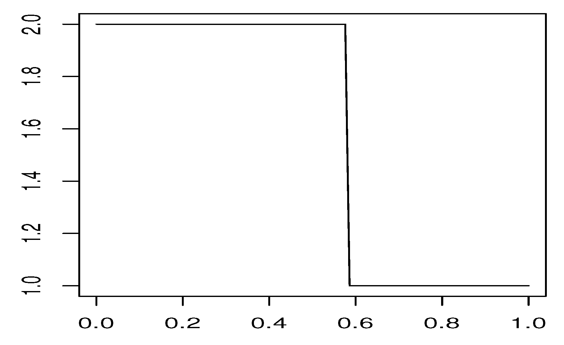
The Figure 4 illustrates the choice of the optimal action for the state $p=3$ depending on the believe state depicted in the same way as in Figure 3. Again the end points of the graph represent optimal actions conditioned on certainty about the current regime. As expected, the optimal decision switches from $a=2$ (act) to $a=1$ (be idle) at some believe probability of approximately $0.55$.

7. Conclusions

Having utilized a number of specific features of our problem class, we suggest a simple, reliable, and easy-to-implement algorithm that can provide a basis for rational sequential decision-making under uncertainty. Our results can be useful if there are no historical data about what could go wrong, or when high requirements on risk assessment are proposed. In such situations, we suggest encoding all relevant worst-case scenarios as potential regime changes, making conservative a priori assumptions on regime change probabilities. Using our algorithm, all optimal strategies can be efficiently examined in such a context, giving useful insights about parameter sensitivity and model risk associated with this sensitivity. The author believes that the suggested algorithm can help gaining a better understanding of risks and opportunities in such context.

References

- Puterman, M. Markov Decision Processes: Discrete Stochastic Dynamic Programming; Wiley: New York, NY, USA, 1994. [Google Scholar]
- Smallwood, R.D.; Sondik, E.J. The Optimal Control of Partially Observable Markov Processes over a Finite Horizon. Oper. Res. 1973, 21, 1071–1088. [Google Scholar] [CrossRef]
- Hinz, J.; Tarnopolskaya, T.; Yee, T. Efficient algorithms of pathwise dynamic programming for decision optimization in mining operations. Ann. Oper. Res. 2020, 286, 583–615. [Google Scholar] [CrossRef]
- Tsiropoulou, E.E.; Kastrinogiannis, T.; Symeon, P. Uplink Power Control in QoS-aware Multi-Service CDMA Wireless Networks. J. Commun. 2009, 4. [Google Scholar] [CrossRef]
- Huang, X.; Hu, F.; Ma, X.; Krikidis, I.; Vukobratovic, D. Machine Learning for Communication Performance Enhancement. Wirel. Commun. Mob. Comput. 2018, 2018, 3018105:1–3018105:2. [Google Scholar] [CrossRef]
- Bäuerle, N.; Rieder, U. Markov Decision Processes with Applications to Finance; Springer: Heidelberg, Germany, 2011. [Google Scholar] [CrossRef]
- Powell, W.B. Approximate Dynamic Programming: Solving the Curses of Dimensionality; Wiley: Hoboken, NJ, USA, 2007. [Google Scholar]
- Belomestny, N.; Kolodko, A.; Schoenmakers, J. Regression methods for stochastic control problems and their convergence analysis. SIAM J. Control Optim. 2010, 48, 3562–3588. [Google Scholar] [CrossRef] [Green Version]
- Carriere, J.F. Valuation of the Early-Exercise Price for Options Using Simulations and Nonparametric Regression. Insur. Math. Econ. 1996, 19, 19–30. [Google Scholar] [CrossRef]
- Egloff, D.; Kohler, M.; Todorovic, N. A dynamic look-ahead Monte Carlo algorithm. Ann. Appl. Probab. 2007, 17, 1138–1171. [Google Scholar] [CrossRef] [Green Version]
- Tsitsiklis, J.N.; Van Roy, B. Regression Methods for Pricing Complex American-Style Options. IEEE Trans. Neural Netw. 2001, 12, 694–703. [Google Scholar] [CrossRef] [Green Version]
- Tsitsiklis, J.; Roy, B.V. Optimal Stopping of Markov Processes: Hilbert Space, Theory, Approximation Algorithms, and an Application to Pricing High-Dimensional Financial Derivatives. IEEE Trans. Automat. Contr. 1999, 44, 1840–1851. [Google Scholar] [CrossRef] [Green Version]
- Longstaff, F.; Schwartz, E. Valuing American options by simulation: A simple least-squares approach. Rev. Financ. Stud. 2001, 14, 113–147. [Google Scholar] [CrossRef] [Green Version]
- Ormoneit, D.; Glynn, P. Kernel-Based Reinforcement Learning. Mach. Learn. 2002, 49, 161–178. [Google Scholar] [CrossRef] [Green Version]
- Ormoneit, D.; Glynn, P. Kernel-Based Reinforcement Learning in Average-Cost Problems. IEEE Trans. Automat. Contr. 2002, 47, 1624–1636. [Google Scholar] [CrossRef]
- Fan, J.; Gijbels, I. Local Polynomial Modelling and Its Applications; Chapman and Hall: London, UK, 1996. [Google Scholar]
- Bertsekas, D.P.; Tsitsiklis, J.N. Neuro-Dynamic Programming; Athena Scientific: Nashua, NH, USA, 1996. [Google Scholar]
- Kaelbling, L.P.; Littman, M.L.; Cassandra, A.R. Planning and acting in partially observable stochastic domains. Artific. Intell. 1998, 101, 99–134. [Google Scholar] [CrossRef] [Green Version]
- Lovejoy, W.S. Computationally Feasible Bounds for Partially Observed Markov Decision Processes. Operat. Res. 1991, 39, 162–175. [Google Scholar] [CrossRef]
- Shani, G.; Pineau, J.; Kaplow, R. A survey of point-based POMDP solvers. Autonom. Agents Multi-Agent Syst. 2013, 27, 1–51. [Google Scholar] [CrossRef]
- Pineau, J.; Gordon, G.; Thrun, S. Point-based value iteration: An anytime algorithm for POMDPs. In Proceedings of the 18th International IJCAI’03: Joint Conference on Artificial Intelligence, Acapulco, Mexico, 9–15 August 2003; pp. 1025–1032. [Google Scholar]
- Hinz, J. Optimal stochastic switching under convexity assumptions. SIAM J. Contr. Optim. 2014, 52, 164–188. [Google Scholar] [CrossRef]
- Hinz, J.; Yap, N. Algorithms for optimal control of stochastic switching systems. Theor. Prob. Appl. 2015, 60, 770–800. [Google Scholar] [CrossRef] [Green Version]
- Hinz, J.; Yee, J. Optimal forward trading and battery control under renewable electricity generation. J. Bank. Financ. 2017. [Google Scholar] [CrossRef] [Green Version]
- Hinz, J.; Yee, J. Stochastic switching for partially observable dynamics and optimal asset allocation. Int. J. Contr. 2017, 90, 553–565. [Google Scholar] [CrossRef]
- Hinz, J.; Yee, J. Rcss: R package for optimal convex stochastic switching. R J. 2018. [Google Scholar] [CrossRef] [Green Version]
- Hinz, J.; Yee, J. Algorithmic Solutions for Optimal Switching Problems. In Proceedings of the 2016 Second International Symposium on Stochastic Models in Reliability Engineering, Life Science and Operations Management (SMRLO), Beer Sheva, Israel, 15–18 February 2016; pp. 586–590. [Google Scholar] [CrossRef]
- Buongiorno, J. Generalization of Faustmann’s Formula for Stochastic Forest Growth and Prices with Markov Decision Process Models. For. Sci. 2001, 47, 466–474. [Google Scholar] [CrossRef]
Figure 1.
Stylized implementation of the control flow within a realistic application.
Figure 2.
Believe state evolution: Observations depicted by red line, the probability that the system is in the regime 2 by black (true state) and blue (filtered believe) line.
Figure 3.
Value function for the state 2 depending on believe probability.
Figure 4.
Optimal action for the state 3 depending on believe probability.