Improving the Robustness of AI-Based Malware Detection Using Adversarial Machine Learning

Abstract

Cyber security is used to protect and safeguard computers and various networks from ill-intended digital threats and attacks. It is getting more difficult in the information age due to the explosion of data and technology. There is a drastic rise in the new types of attacks where the conventional signature-based systems cannot keep up with these attacks. Machine learning seems to be a solution to solve many problems, including problems in cyber security. It is proven to be a very useful tool in the evolution of malware detection systems. However, the security of AI-based malware detection models is fragile. With advancements in machine learning, attackers have found a way to work around such detection systems using an adversarial attack technique. Such attacks are targeted at the data level, at classifier models, and during the testing phase. These attacks tend to cause the classifier to misclassify the given input, which can be very harmful in real-time AI-based malware detection. This paper proposes a framework for generating the adversarial malware images and retraining the classification models to improve malware detection robustness. Different classification models were implemented for malware detection, and attacks were established using adversarial images to analyze the model’s behavior. The robustness of the models was improved by means of adversarial training, and better attack resistance is observed.

1. Introduction

Malware has been a threat to individuals and organizations for a very long time. It dates back to the 1970s, when the Creeper Virus was first encountered. Since then, the world has faced a constant and never-ending stream of malware attacks from hundreds of thousands of its variants [1,2]. The sole intent of such programs is to cause as much disruption and destruction as possible [3,4,5]. Even after advancements in cybersecurity, malware attacks are still a great threat to the world. Recent studies have shown that more than 60% of organizations still face malware threats, and just 5% of companies’ documents are properly protected, on average. These dangers cost a lot of money and time, with the average cost of a malware assault on a corporation being USD 2.6 million and the average time it takes to recover from a malware attack being 50 days [6,7]. Machine learning in malware detection has become increasingly important in the face of such serious attacks.

Every day we face a new threat in cyberspace. With the onslaught of such threats, we need a tool to go toe to toe with it [8,9]. Machine learning is the answer to not just this but many other problems [10]. Even though today’s systems are built with some of the most secure code and penetrate systems, there are still many vulnerabilities, primarily due to human error, obsolete software, and the use of insecure protocols and systems. Malware is the modern-day artillery used by attackers to hurt unsuspecting consumers and steal their data by violating their privacy [11,12]. Malware detection systems have progressed from detecting binary files to detecting executables. However, such attacks can also target the detection system [13].

Machine learning models learn to classify malware by a learning process in which the model is provided with a training data set and testing data set. The model learns with the help of the training dataset [14,15]. There is a huge drawback to this approach. The attackers can affect the learning process and circumvent the classifiers, helping them to bypass the detection systems. It also affects the privacy preservation of the data in such systems [9,16]. Along with machine learning, deep learning techniques have also been applied to improve malware detection’s accuracy [17]. DL models such as LSTM, RNN, CNN have been implemented in the literature [18,19].

Adversarial attacks are these types of attacks, and adversarial modeling (AML) is the process of training a model to withstand them without compromising its overall effectiveness (adversarial machine learning) [20,21]. It has been extensively tested and applied in areas such as spam detection and image classification. In domains such as malware detection, its exploration is currently insufficient [22,23]. Robust malware detection is not only needed for standalone systems, but also IoT-based systems [24,25] and Android systems, which also require an aggressive malware management framework. Lots of attacks happen at the sensor level, and also in Android-based devices [26].

In this work, the authors examined various state-of-the-art ML and DL architectures and their optimization for malware detection in this research work, and how those algorithms may be made more robust by attacking and training them using adversarial data.

2. Theoretical Background

2.1. Malware and Types of Malware

Malware is malicious software that causes extensive damage to the data and systems or gains access to the sensitive information of a network. Based on its purpose, malware classification can be performed in the following ways.

2.2. Malware Analysis

Before initiating malware detection techniques, there is a need to analyze the different functionalities of a particular malware, how it executes these functionalities, and the purpose behind its development. Malware analysis techniques are classified into three main categories [27]:

• Statics Analysis—This includes examining a program’s or software’s source code without running it. The static information from the source code is extracted in this procedure to see if it contains any dangerous code. Debuggers, de-compilers, de-assemblers, code analyzers, and other tools are used for this type of analysis. File format extraction, string extraction, fingerprinting, AV scanning, and disassembly are some of the methods used to do perform static analysis with the help of these tools.
• Dynamic Analysis—The functionality of the software or a program is examined using this method, which involves running the source code. In other words, a software’s behavior is examined, and the software’s intents or purpose are deduced from these observations. This is commonly done in a virtual environment with a sandbox, simulator, emulators, RegShot, a process explorer, and other tools. This strategy makes malware detection simple.
• Hybrid Analysis—This is a hybrid of static and dynamic analysis techniques. The source code is first analyzed in this manner, and then it is run in a virtual environment to examine its actual behavior [28].

  Table 1. Comparison between static analysis and dynamic analysis.

  Static Analysis	Dynamic Analysis
  Signature-based malware detection	Behavior-based malware detection
  Simple and Straightforward analysis	Thorough analysis
  Best suited to detect common malware	Can detect advanced malware
  It is fast and safe	It is time-consuming and vulnerable

  shows the comparative analysis of static and dynamic methods.

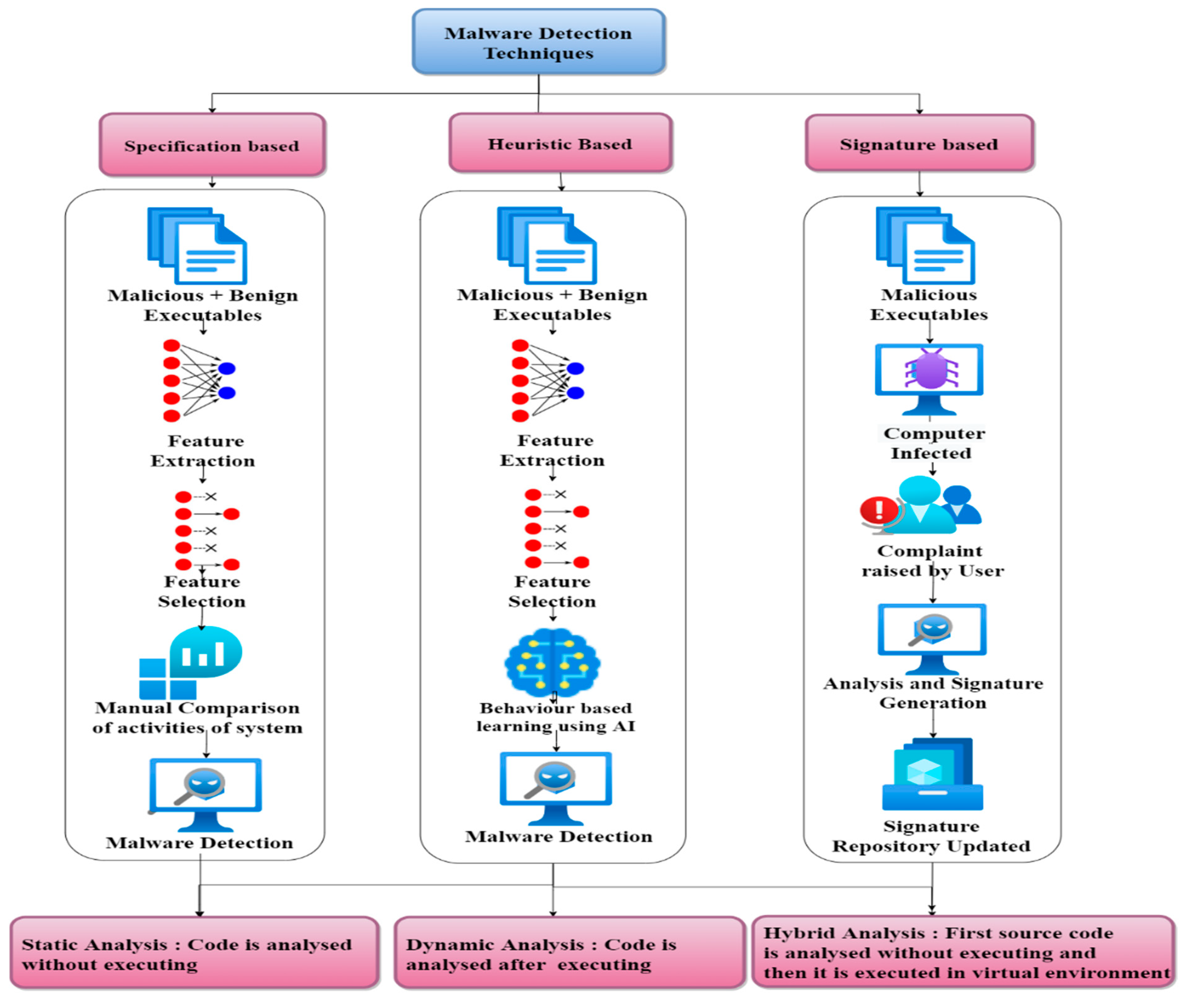
2.3. Malware Detection Techniques

Malware detection strategies can be divided into three categories based on signatures, heuristics, and requirements. These strategies describe and track malware, as well as taking countermeasures against it, to safeguard information systems, data, and resources from being harmed by it [27]:

• Signature-based detection technique: When malware is created, it has a signature, which may determine which malware family it belongs to. The majority of antivirus solutions use a signature-based identifying mechanism. The antivirus software decodes the corrupted file code and looks for malware-related sequences. Signatures of malware are stored in a database and are compared later during the detection process. This type of identification technique is also known as scanning or matching string or pattern. It could be static, dynamic, or hybrid in nature.
• Heuristic-based detection technique: Heuristic-based identification detects or distinguishes between a system’s normal and abnormal activities, allowing known and suspected malware threats to be identified and resolved. The heuristic-based detection technique is divided into two parts. In the first stage, the behavior of the mechanism is observed in the absence of an attack, and a record of essential details is kept that may be confirmed and tested in the event of an assault. This disparity is noted in the second phase to detect malware from a certain family. The action detector in the heuristic-based methodology is made up of the three basic components listed below.

  (a)

  Data collection: Under this component, the data collection is performed with either static or dynamic techniques.

  (b)

  Interpretation: This component turns the data obtained by the data collection component into the intermediate form after interpretation.

  (c)

  Matching algorithm: This component is used to match the transformed information to the behavior signature in the interpretation component.

• Specification-based detection techniques: Applications are managed according to their parameters and controls for normal and abnormal behavior in specification-based detection approaches. This methodology is derived from a heuristic technique. The key difference is that heuristic detection techniques use machine learning and AI to identify a legitimate program’s valid and invalid behavior. In contrast, specification-based detection techniques study the actions defined in the system specification. This method is more of a manual comparison of the system’s typical operations. It solves the flaws of heuristic-based techniques by lowering the number of false positives and increasing the number of erroneous negatives. Each malware detection technique might be static, dynamic, or hybrid. Figure 1 shows an overview of the different malware detection techniques.

2.4. Need for Artificial Intelligence

Malware detection systems based on signatures work flawlessly when the malware is previously known and has been detected by some other antivirus vendors. However, such a system is practically useless in polymorphic malwares, as they would go undetected because such malware can change their signatures. So generally, malware detection depends on the heuristic-based approach for such kinds of malware. However, it is not very efficient in adequately detecting malware, as it gives many false positives and false negatives.

Now, the spread of such polymorphic malware has overwhelmed the traditional heuristic-based approach. One solution to this problem is to amalgamate the heuristic-based approach and the powers of machine learning methods [29] to yield higher accuracy during the detection.

3. Malware Detection and Classification with Machine Learning

Machine learning is a methodology in which we make the computer learn about the problem statement. We make it learn by giving it the data and the information in observation and real-world interactions. In the architecture of malware detection proposed by Gupta et al. [30], they used data from the VXheaven, Nothing, and VirusShare datasets on models and applied 10-fold cross-validation to it. Multiple classification algorithms were used, including support vector machine, naive Bayes and random forest. The performance was evaluated using the FPR, FNR, TPR, accuracy and precision. The naive Bayes, SVM, and random forest gave the accuracy of 96.8%, 97.68%, 99.11%, respectively [31]. Among the three, random forest showed the highest accuracy, with the lowest FPR & FNP.

Burnap et al., 2018 [32] presented a novel approach where the self-organizing feature maps are used to classify and reduce the overfitting between the malware and benign files occurring during training of the dataset. This dataset is gathered with the help of the VirusTotal API. Random forest, BayesNet, MLP, and SVM are among the classifiers used in this paper. The random forest classifier has the highest accuracy, with a score of 98 percent. However, due to overfitting, it was reduced by 12% when applied with various datasets. The problem of overfitting was addressed with the program Self-Organizing Feature Map (SOFM), which is a classifier based on the ANN technique, and the accuracy increased by 7%.

Al Ahmadi et al., 2018 [33] suggested a novel mal classifier technique. CTU13 and the Stratosphere IPS project were the datasets used. With 95.5 percent accuracy, KNN and Random Forest were employed for malware classification and training.

Pai et al., 2017 [34] proposed a novel malware classification method based on clustering techniques such as k-means, expectation-maximization, and hidden Markov models. The information was gathered from the Malicia website. Among all of the methods, expectation-maximization had the best accuracy.

Liu et al. [35] provided an approach in which the unknown malware instances are classified into a cluster according to their families. The shared nearest neighbor clustering algorithm was used, giving an accuracy of 98.9% for available malware and 86.7% for unavailable malware.

Neural networks were employed by Kosmidis et al., 2017 [36] to classify unknown malware. The methods used for malware classification were perceptron, decision tree, closest centroid, stochastic gradient, multilayer perceptron, and random forest, with the random forest approach providing the best average of training and testing accuracy.

Gandotra et al., 2014 [37] presented a framework to classify unknown malware extracted from static and dynamic features. Multilayer perceptron, IB1, decision tree, and random forest were the four classifiers used to classify the data. With a 99.58 percent accuracy rate, random forest was the most accurate.

Tian et al., 2009 [38] proposed a method for classifying malware using printable strings. Naive Bayes, support vector machine, IB1, random forest, and decision trees were used on the retrieved features. The AdaBoostM1 meta-classifier was employed to increase efficiency. With a 97 percent accuracy, random forest and IB1 produced superior outcomes.

Devesa et al., 2010 [39], To improve the performance, Naive Bayes, SMO, Random forest and J48, were used to the retrieved features in this work. Random forest classifiers were the most accurate, with a 96.2 percent accuracy rate.

4. Challenges

Detection systems empowered by machine learning usually react to evasion attacks by analyzing the attack and retraining the model based on the newly collected data. The next time the attacker uses a similar approach, the system can counter the attacker’s strategy. This system works fine in the scenario mentioned above, but what if it is under attack? A type of attack that feeds the system with an example that makes the model learn to misclassify? Such types of attacks are known as adversarial attacks, and are an increasing threat in the security area. Such a challenge can be overcome by none other than what is called adversarial machine learning [40].

Table 2. Overview of existing techniques.

Paper	Algorithms Used	Dataset Sources	Results
[30]	Naive Bayes methodology, SVM, random forest	VX Heaven, Virus, Share, Nothin K.	The Random Forest gives the best accuracy
[32]	Random forest, BN, MLP, SVM, SOFM	Virus total AP	Performance increased by 7.24% to 25.68%
[33]	KNN, random forest	CTU13, Stratosphere IPS project	Performance increased. An accuracy of 95.5% was accomplished
[34]	Clustering algorithms	Collected from Malicious website	Expectation maximization techniques give a high accuracy
[35]	Shared nearest neighbor (SNN)	Kingsoft, ESET NOD3 2, and Anubis	98.9% accuracy of known malware and 86.7% of accuracy for unknown malware detected
[36]	Stochastic gradient, multilayer perceptron, random forest, decision tree, nearest centroid and perceptron	Making a dataset	Improved accuracy results using random forest algorithms
[37]	MLP, DT, IB1, random forest	University of California	Random Forest had high accuracy values of 99.58 percent
[38]	Random forest, IB1, DT, support	CA’s (Computer Associates) VETZoo	Better accuracy and improved performance by 9% using random forest
[41]	Ada Boost, IB1, random forest, support vector machine, DT, naive Bayes	CA’s VET zoo	Overall classification accuracy is 97%
[39]	Naive Bayes, random forest, SMO, J48	VX Heaven	Random Forest gave high accuracy of 96.2%

shows an overview of the existing systems and also discusses the AI algorithms used in these systems.

5. Adversarial Machine Learning

Machine learning algorithms are developed to assume that the environment is benign, but they fail when even a small adversary can modify their inputs. This is where adversarial machines come in handy [42]. Adversarial machine learning is a branch of machine learning that studies a set of assaults aimed at degrading the performance of classifiers on certain tasks. Adversarial machine learning ensures the machine learning model’s resilience [22,43]. Figure 2 and Figure 3 show the taxonomy of the adversarial attacks and defenses.

5.1. Adversarial Attacks

Several attack tactics and approaches have been studied and utilized to identify malware, with a trade-off between several characteristics, including performance, complexity, computing efficiency, and application situation, including black box and white box assaults [44]. White box attacks are those in which the attacker has all the information and know-how about the internal workings of that particular model, including training data, model parameters, and other useful information about the classifier. In contrast, black-box attacks are those in which the attacker cannot or does not know the internal workings of the model and has no prying access to it.

On the other hand, gradient-based techniques frequently include certain perturbations that are specifically developed and optimized for specific distance metrics between the original input samples and the perturbed ones.

The following are three frequently used distance measures that have been studied in the literature:

• Linf—This effectively reduces the maximum amount of disturbance that every feature is subjected to;
• L0—On the other hand, this reduces the number of characteristics that are affected;
• L2—This lowers the ED between the initial and altered samples on average.

Different Adversarial Attacks

• L-BFGS: This attack method uses the L2 Distance Metric. To reduce the number of perturbations applied to the pictures, the L-BFGS optimization is utilized [20]. This approach is quite good at generating adversarial instances. However, it is computationally rigorous, because this attack approach is categorized as an optimization method with box constraints.
• FGSM: This assault technique uses the Distance Metric LinF. In this assault technique, flat perturbations are applied to every feature in the direction of the gradient. This assault technique saves time in terms of computing. The main disadvantage of this assault approach is that perturbations are produced even when they are not needed and are applied to every feature.
• JSMA: This assault tactic uses the Distance Metric L0. Flat perturbations are applied to features in decreasing order in this attack approach, depending on their saliency value. Because just a few characteristics are disrupted, this attack technique is highly successful. It is, nevertheless, more computationally expensive than FGSM.
• Deepfool: Distance Metric L2 is used for this attack strategy. This attack strategy estimates decision boundaries between the classes, and the perturbations are added iteratively. This strategy is highly effective at producing adversarial examples. This strategy, however, is computationally more intensive than FGSM and JSMA, and adversarial examples likely produced may not be optimal.
• C&W: This assault plan employs all distance measurements, L0, L2, and Linf. This attack technique is similar to the L-BFGS attack (i.e., optimization problem), except it does not need box restrictions and has different objective functions. Although this method is computationally more rigorous and demanding than other attack tactics, such as FGSM, JSMA, and Deepfool, it is highly successful at creating adversarial instances and can quickly overcome various adversarial defenses.
• GAN/WGAN: This assault tactic employs no distance metric. This approach entails training two neural networks, one for generating samples and the other for distinguishing between actual and produced samples. This approach is quite good at producing samples that are not the same as those used in training. However, training a GAN requires a lot of computing power and can be quite unstable.
• ZOO: This assault tactic uses the Distance Metric L2. This approach predicts the gradient and hessian by querying the target model with updated individual characteristics and utilizing Adam or Newton’s technique to minimize perturbations. Its effectiveness is comparable to that of the C&W assault. This assault strategy’s sole disadvantage is that it necessitates a high number of requests to the target classifier.

5.2. Adversarial Defenses

• Adversarial Training: This method integrates hostile instances (adversarial example) into the training set or the model’s loss function, making it easy to use. When assaults during deployment are identical to those in training, it is the most successful defense technique. The only downside is that this method requires retraining the classifier in use, and it may be ineffective against assaults not listed above [20].
• Gradient Masking: This entails employing strategies that cause the attacker to become perplexed regarding the model’s gradient, causing them to underestimate it. If attacks are transferable across various models, this defense technique will fail.
• Defensive Distillation: This requires creating and training a new network with the last structure, using neural network distillation. However, the C&W attack appeared to have defeated them. Aside from that, it necessitates the training of a completely new model, which is another drawback of this defense.
• Feature Squeezing: This is a collection of techniques that classify data using compressed characteristics and features. It is best for working with images because it is only beneficial in specific cases where compression is achievable without considerable data loss.
• Transferability Block: As part of this defense mechanism, the model is trained with new labels (NULL) with values proportional to the amount of noise in the sample. This is one of the most effective strategies for finding conflicting instances. It is, on the other hand, unable to recognize an antagonistic sample’s original labels.
• Universal perturbation defense method: This method employs a network that takes features from adversarial instances and trains another model that recognizes and identifies these adversarial samples. This does not necessitate the training of new models and works in the same way as other defense mechanisms, but attacks with different parameters can have identical effects.
• MagNet: With reconstruction error, this method trains an autoencoder to recognize adversarial examples and then utilizes a different one to produce non-adversarial samples for classification on a separate classifier. It necessitates autoencoders, which might be difficult to train at times, which is a disadvantage of this technique.

A malware detection approach based on autoencoders and GANs was proposed by Jin-Young Kim et al. [45]. They used a typical malware challenge dataset that was accessible on Kaggle. In identifying adversarial assaults, their suggested model beat models of machine learning used in the past, such as support vector machines, KNN, random forest, MLP, and naive Bayes. Joseph Clements et al. used the Kitsune network IDS (NIDS) classifier on the Mirai botnet dataset to detect malware using four adversarial attacks: FGSM, ENM, JSMA, and C&W.

Their study’s primary findings were that all attacks had 100% FNR in integrity attack scenarios. In comparison, JSMA and FGSM only had 4% and 0% FNR in availability attacks, respectively, while C&W and ENMc had 100 percent.

Biggio et al. [46] created various adversarial cases and tested them against malware classifiers for PDF files using the Contagion dataset. Both neural networks and SVM classifiers obtained false negative rates of up to 100%, suggesting that the assaults were extremely successful in a black-box scenario.

In a black-box oracle setting, Weiwei Hu and Ying Tan employed MalGAN to create adversarial malware. The classifiers addressed included random forest, linear regression, decision tree, SVM, MLP, and a voting ensemble of the preceding classifiers. The study discovered that all classifiers could achieve a TPR of 90%, with decision trees performing the best. All classifiers’ TPRs went below 0.20 percent.

Grosse et al. [47] discovered that the attack employing the Drebin dataset, an Android malware dataset using a binary neural network classifier, had misclassification rates ranging from 63 to 69 percent, with decreased misclassification rates as the malware ratio increased. The distillation and adversarial training techniques were also tested, with results indicating that accuracy decreased by up to 2% while using distillation on normal data. Still, the misclassification rate plummeted by up to 38% when under assault.

Anderson et al. [48] used a reinforcement learning technique, deep Q-learning, to target a malware dataset. When a sample successfully misclassified the target model, it was given this reward. The authors utilized a gradient augmented decision tree to tackle it, which yielded a 16 percent evasion rate. Their findings also indicate the characteristics which were used to attack the model.

Weilin Xu et al. [49] employed a genetic programming technique to conduct evasion attacks on the Contagio PDF malware dataset. The results indicate that a 100% evasion rate was obtained while assaulting both defenses and maintaining the integrity of all attacks. In all, 16,985 evasive variants for PDFrate and 2859 for Hidost were identified.

Calleja et al. [50] employed genetic programming techniques to change dangerous Android apps in the DREBIN dataset so that they were mislabeled to distinct malware families, and then used RevealDroid, a decision tree-based categorization tool. The authors were able to misclassify 28 of the 29 malware families by only adding one additional feature.

Menéndez et al. [51] utilized entropy time series analysis with different forms of polymorphism (EnTS). The Kaggle malware competition dataset, packet (Pck) malware from VirusShare, and Mix, a dataset created from the first two, were used to evaluate the method. According to the data, EnTS achieved 82 percent accuracy while maximizing precision (100 percent) and 93.9 percent accuracy while maximizing accuracy. El Empaquetador Evolutivo (EEE) assaults resulted in an FNR of 90.8 percent to 98.7 percent, up from 0% to 9.4% without attacks.

Chen et al. [52] proposed evasion attack malware (EvnAttack) situated in exec and enhanced the FNR from 0.05 to 0.70. In addition, when Se Defender was deployed, the F1 score was restored to 0.95, while the FNR was drastically lowered.

Anderson et al. employed GANs for DGA, commonly used by malware to allow numerous created domains to update the infection. After training the auto-encoder on the Alexa top 1M dataset, a random forest classifier with specifically built properties such as length, entropy character distribution, and vowel to consonant ratio was used.

This table files CCSCD (private) was used, and the results showed that Even Attack dropped the F1 score from 0.96s to 0.43s model decreased AUC against regular attacks from 0.99 to 0.94.

Table 3. Overview of existing adversarial attack techniques.

Paper	Attack Techniques	Classifiers	Datasets	Metrics	Results and Conclusion
[45]	GAN	Decision tree Random forest SVM KNN Naive Bayes LDA	Kaggle Malware VirusShare	Accuracy	-An accuracy of 98% was reached when other techniques were only able to reach between 66% and 96% accuracy.
[53]	FGSM JSMA C&W ENM	Kitsune NIDS (ensemble of autoencoders)	Mirai botnet	False-negative rate	-All attacks were able to achieve 100% FNR. -Under availability attacks, FGSM and JSMA were only able to achieve 0% and 4% FNR, while C&W and ENM were able to achieve 100%.
[46]	Gradient-Based Technique	SVM Neural Network	Contagio	FNR	-FNR for NN and SVM classifiers reached 100%. -In a black-box setting, the attacks are quite effective.
	GAN	Neural network	malware	TPR	-TPRs of more than 90% were achieved by all classifiers, with the decision tree proving to be the strongest performer. TPRs for all classifiers fell below 0.20 percent.
[47]	Modified JSMA	Neural network	DREBIN	Misclassification rate	-under attack misclassification rate was between 63% and 69% -Distillation reduced the accuracy by 2% but improved MR to 36%
[48]	Deep Q-Learning	Gradient boosted DT	Custom	False-negative rate	-For the black box attack, a 16 percent evasion rate was attained.
[49]	Genetic Algorithm	PDFrate (Random forest) Hidost (RBF SVM)	Contagio	Evasion rate	-An evasion rate of 100% was recorded against both defences -16,985 evasive variants were found for PDF rate and 2859 for Hidost
[50]	Genetic Algorithm	RevealDRoid (Decision tree)	DREBIN	Evasion rate	-For 28 of the 29 malware families, a 100 percent evasion rate was obtained.
[51]	El Empaquetador Evolutivo	Entropy time series analysis	Kaggle Malware VirusShare	Precision Accuracy False-negative rate	-EnTS was able to attain an accuracy of 82 percent and 94 percent when maximizing accuracy. When using EEE, the false negative rate increased from 0% to 9.4 percent, but the rate increased from 0% to 9.4 percent when not using EEE.
[52]	EvnAttack	Unspecified	Comodo Cloud Security Centre Dataset (Private)	F1 score, FNR	-EvnAttack improved the FNR from 0.05 to 0.70 and reduced the F1 score from 0.96 to 0.43. -Se Defender improved the F1 score from 0.43 to 0.95 while also significantly lowering the FNR.
[54]	GAN	Random forest	Alexa top 1M domain	AUC	-A decrease in the AUC from 0.99 against regular attacks to 0.94 against GAN was noted.

gives an overview of the existing adversarial attack techniques.

6. Implementation

6.1. Proposed Flow of Research Work

Based on the literature review and the knowledge acquired, the authors proposed the methodology as explained in Figure 4.

6.2. Data Collection

About the Dataset

As the first step of data collection, we first finalized an open-source malware dataset called the MaleVis dataset [55]. It comprises byte images of 25 malware classes and one legitimate class. This dataset was constructed by converting malware binary files into three-channel RGB images using bin2png script developed by Sultanik. This dataset is available in two square-sized resolutions, that is, 224 × 224 and 300 × 300 pixels.

The MaleVis dataset has a total of 9100 training and 5126 validation RGB images. All the classes in the training set are perfectly balanced, containing 350 images each. While the validation set has a varying number of images. However, the legitimate class in the validation set is larger, having 1482 images. This is because the nature of malware detection is based on discriminating the legitimate ones from the malware images. Figure 5 shows the different malware classes in the Malevis dataset, Figure 6 shows the distribution of samples across various malware classes loaded in the datasets. Figure 7 shows the classification of different malware classes into malware types.

Bozkir et al. [56] proposed a new memory dumping and computer vision-based method to detect malware in memory even they do not exist on hard drive using MaleVis dataset. The state of the art manifold learning and dimension reduction technique named UMAP was used for the first time in the problem domain for better discrimination.

Aslan et al. [57] proposed a novel hybrid deep-learning based architecture for malware classification with the help of the MaleVis dataset. The authors’ suggested method uses a new hybrid layer that involves two pre-trained models instead of one model. The proposed method reduces feature spaces significantly. The measured accuracy rates are higher than those of known methods.

6.3. Algorithms Used

The authors used three different types of classification algorithms as explained.

6.3.1. Machine Learning

Random forest [58] is a machine learning approach based on ensemble learning, which is described as a way for addressing a complex issue by integrating several classifiers and then improving the model’s performance.

It is a classifier that utilizes the arithmetic mean to improve the dataset’s prediction accuracy. It is a classifier with a lot of decision trees based on distinct subsets of the original dataset.

The random forest algorithm’s operation may be summarized as follows:

• K random data points are chosen at random from the dataset.
• The decision trees that are related to the specified data points are built.
• Choose the number N for the decision trees that need to be built.
• Repeat steps 1 and 2 as needed.
• Finally, calculate the new data points’ forecasts for each tree, and then assign the new data points to the category with the highest votes [59,60].

6.3.2. Deep Learning

Deep learning is a type of machine learning. We can extract greater features from input data using a deep network of artificial neurons and artificial neural networks. Deep learning starts working with the raw data, from the lowest level then works its way to the higher levels. For instance, in image classification, the lower levels would detect the edges of the object in the image, and as the neural network gets more complex, it may take on high-level features. There are many different deep learning algorithms for different sorts of challenges. The authors chose the convolutional neural network for this research work. Figure 8 shows the architecture of the CNN model.

Convolutional Neural Networks

Convolution is the process of applying a filter to an input to generate an activation. When the same filter is applied several times, a feature map is created, indicating the position and intensity of identified features in input, such as an image. What distinguishes CNN is its ability to learn many filters in parallel, specifically to a training dataset, within the constraints of any specific classification or prediction modeling job, such as image classification. As a result, the input image has a collection of very distinct characteristics that may be easily identified [61,62].

EfficientNet B0

In computer vision, transfer learning is a popular method, since it allows quick development and building accurate and efficient models. Instead of starting the learning process from scratch, transfer learning begins with patterns learned while solving a separate problem. This way, one can build on existing knowledge rather than starting from scratch [30].

Pre-trained models are commonly used to implement transfer learning. A pre-trained model has been trained on a big benchmark dataset to tackle a problem comparable to the one that one decides to work on. As a result of the high computational cost of training such models, it is customary to import and use models from the literature (e.g., VGG, Inception, MobileNet). In this research analysis, the authors implemented the EfficeintNet- B0 model to detect malware.

EfficientNet-B0 is a CNN architecture and a scaling method that evenly scales all dimensions, including depth/width/resolution, using a compound coefficient. For example, if we choose to use computational resources that are 2^N times larger, then this can be done by increasing the depth of the network by ɑ^N, the width of the network by β^N, and image sizer by ɣⁿ, where ɑ, β, and ɣ are all constant coefficients. The implementation of EfficientNet-B0 is performed by using the imagenet weights.

6.4. Adversarial Sample Generation

A variety of deep learning algorithms are highly accurate and precise in classification tasks, be it natural language or image. These models are considered to be very good in terms of their performance. However, at the same time, various research and studies claim that these models, without any prior specific training, are highly susceptible to adversarial attacks. With an increase in the research in AML, a variety of new and much more powerful algorithms have been developed, which could easily temper and exploit these models [63]. In many scenarios, the attacks are initiated and implemented using the adversarial samples created and given to the models to implement an attack, as shown in Figure 9. In some cases, these samples are designed not to be visible to the naked eye, and one cannot figure out any difference.

These attacks are divided into two categories: white-box attacks, in which the attacker has complete control and knowledge of the model’s structure before initiating and implementing attacks, and black-box attacks, in which the attacker does not have complete control and knowledge of the model’s structure before initiating and implementing attacks.

The fast gradient sign method is a type of white box attack and uses adversarial samples to implement an attack to temper and exploit a given model. An adversarial image needs to be created to implement this attack. Adversarial images are created using the combination of input (normal image) and a perturbation. These perturbations are the noises added to an input image to create an adversarial image [64,65]. In FGSM, the perturbations are created using the input samples. Thus, each perturbation is unique for different input samples and is generated by analyzing the different properties of the samples. This process causes the perturbations to completely merge into the input image so that the human eye cannot figure out the difference between the original and the perturbed image [66].

A simple schematic representation of how the FGSM algorithm works can be seen from the example below.

The FGSM method works in the following manner:

• Take an input image
• Make predictions using a trained model on the image
• Computation of loss of prediction based on the true class label
• Calculations of the gradients of loss for the input image
• Computation of the sign of the gradient
• Use the signed gradient to construct the output adversarial image

For this work and research analysis, to generate the adversarial images for the Malevis dataset, the steps mentioned in the algorithm were used. Several input images were grouped in batches based on the class of the images and were taken as samples and put through the FGSM model for various epsilon values. Subsequently, the adversarial samples were generated. The three epsilon values used for the sample generation for this project and research were 0.01, 0.1 and 0.15. Epsilon values are values multiplied by the signed gradients to ensure that the perturbations are small enough that the human eye cannot detect them but are large enough to fool the trained models.

Table 4. Adversarial input generation.

Classes	Original Input	Adversarial Inputs
		ε = 0.01	ε = 0.1	ε = 0.15
installCore
Elex
VBA
Neoreklami
Amonetize
Vilsel
Autorun
Hlux
Expiro
BrowseFox

shows the generation of adversarial input malware images at various epsilon values.

6.5. Adversarial Defense Mechanism

The below schematic representation shows how the authors performed the adversarial attack. Different models, namely, random forest, convolution neural network and EfficientNet B0, were initially trained using the MaleVis dataset by traditional methods, after which an adversarial attack using the FGSM method was performed. The images in the dataset were mixed with some noise of three different epsilon values, which were 0.01, 0.1, and 0.15. When these adversarial images are fed into the classifiers, they fail to classify them into their proper classes correctly. This can be a threat to the malware detection system, as a malicious file can be classified as a benign file and can cause huge damage to the computer system [32,66].

To mitigate this, an adversarial defense technique made the classifier robust against the FGSM attack. The technique proposed by the authors is an adversarial training defense mechanism. In this technique, the adversarial samples are included in the training set and then fed to the model to learn the different features of adversarial samples and clean images [67]. In various recent studies and articles, this type of defense technique proved to be one of the most effective defensive mechanisms against a particular attack. In this research work, the authors have particularly performed the FGSM adversarial training method, including the adversarial samples generated using the FGSM method explained in the previous section. This can help to improve the error rate on the samples generated using the MaleVis dataset and the FGSM attack [53]. Figure 10 and Figure 11 demonstrate the process of establishing the adversarial attack and defense.

7. Results

7.1. Results Obtained before Performing Adversarial Attacks

The authors compared the results obtained before performing the FGSM attack by training the MaleVis Dataset on the different classification models, i.e., random forest (machine learning), CNN (deep learning), and EfficientNetB0 (transfer learning). The confusion matrix is also given below for each of the classifiers used in work. In these matrices, we can see the number of images getting properly classified and the number of misclassified images for each class.

• Random Forest: The results obtained after the dataset training show that the random forest classifier was able to achieve an accuracy of 93%. The confusion matrix below shows that the classifier could classify the images correctly for classes like Vilsel, where a total number of 71 images were given to the model. It was able to classify them with 100% accuracy, as no image was misclassified into any other class. Along with Vilsel, the images belonging to the Amonetize, Hlux, Neoreklami, Regrun, Sality, and VBA classes were also classified with 100% accuracy. Dinwood and Adposhel followed this with only one misclassified image, whereas images from the Neshta class were highly misclassified. Figure 12 shows the confusion matrix for CNN.
• Convolutional Neural Network (CNN): Convolutional neural network gave an accuracy of 92.3% after training the images from the MaleVis Dataset. The confusion matrix shows that the images belonging to Amonetize, Fasong, HackKMS, Hlux, InstallCore, Regrun, Stantinko, Snarasite, VBA, and Visel were correctly classified by the CNN classifier. Compared to random forest, CNN was able to give 100% accuracy to more classes. The Neshta class of the malware family had the least accuracy. Out of the total 88 images fed into the classifier, only 52 were classified correctly as Neshta, whereas 9 images were classified as benign images and 8 were classified into Sality class. After Neshta, the Expiro class had the least accuracy of 72.22%. Figure 13 shows the confusion matrix for CNN model and Figure 14 displays the training and testing loss curves.
• EfficientNet B0: The model developed using EfficientNet-B0 was able to achieve an accuracy of 93.7%. The classes with 100% accuracy were HackKMS, InstallCore, Multiplug, Regrun, Snarasite, VBA, VBKrypt, and Vilsel. Similar to random forest and CNN, this classifier also performed poorly for Neshta with an accuracy of 64.94%. Figure 15 shows the confusion matrix for the random forest model, and Figure 16 displays the training and testing loss curves.

7.2. Results Obtained after Performing Adversarial Attack

The classifiers that the authors developed were then attacked using the FGSM adversarial attack. Adversarial samples were generated for each class with different epsilon values, namely, 0.01, 0.1, and 0.15, and then were passed into the model to check its behavior against them. Figure 17 shows the results obtained after performing adversarial attack. The results of this attack are explained below.

• Random Forest: The random forest classifier was observed to be relatively more affected by the FGSM attack with an epsilon value of 0.1 and above. With the 0.01 epsilon value of the model, the confidence level was significantly dropped but did not misclassify for maximum classes. There were some classes, such as like Nestha and Other, for which the images were misclassified with a confidence level of 46% and 53%, respectively. The Vilsel class, which was classified with 100% accuracy before the attack, had a confidence level of 68% for the epsilon value of 0.01. The overall accuracy for the class for the epsilon value 0.1 was dropped by around 16% from 100% to 84.52%, whereas the Hlux class’ accuracy was observed to be 83.66%, which was 100% before attack. The attack performed with 0.15 epsilon proved fatal as the average accuracy drop was 40%.
• CNN: Compared with the random forest classifier, CNN was relatively less affected by the attack for an epsilon value of 0.1 and above. Still, for 0.01, it was similar to random forest classifier. Only the confidence level dropped for classes such as Amonetize, Fasong, InstallCore, Regrun, Stantinko, Visel, etc., which had very high accuracy before attack. However, the classes which had very poor accuracy were misclassified even with a 0.01 epsilon value, such as Expiro and Neshta, whose accuracy dropped from 59.09 to 39% and 72.22 to 63.40%, respectively. For an epsilon value of 0.1, the most affected classes were Autorun, whose accuracy dropped from 86.36% to 52.42%, and Neshta, whose accuracy dropped to 31.58%. The accuracy for each class was dropped around 30–35% for the epsilon value of 0.15.
• EfficientNet B0: This classifier proved to be least affected by the attack as compared to the previous two models. Only the Neshta class was seen to have misclassification for 0.01 epsilon values. During the attack with 0.1 epsilon, the classes were significantly impacted in terms of misclassification. The most affected classes were Elex, Expiro, and Other (Benign), with 72.34%, 68.42%, and 70.22% accuracy. As seen earlier in the before the attack section and after attack, Neshta is the only class with the highest misclassification rate for all classifiers developed by the authors. The 0.15 epsilon caused a 30% drop on average in the accuracies of all classes of the dataset.

The graphs of some classes from the MaleVis dataset shown below give a comparative analysis of the effect of the attack for all the three epsilon values on each of the classifiers ε.

7.3. Results Obtained after Performing Adversarial Defense

To make these developed models robust, adversarial training defense techniques were implemented. This involves including the adversarial samples into the dataset and then retraining the model. In this section, the results obtained by performing this defense technique are discussed.

The defense mechanism implemented showed positive results, as the authors were able to raise the accuracy and bring it closer to the accuracy achieved before the Attack. As seen in the table below, the accuracy, F1 score, and precision before the attack and after defense are almost similar, which proves that the authors were successful in making the classifiers robust against the FGSM attack, and if any adversarial image is fed to the classifier again, it would be able to classify it as malware/benign image.

Table 5. Comparative metrics for all models before attack, after attack, and after the defense.

Before Attack
Classes	Random Forest			CNN			EfficientNet B0
	Accuracy (%)	F1-Score	Precision	Accuracy (%)	F1-Score	Precision	Accuracy (%)	F1-Score	Precision
Elex	96.72	0.97	0.97	96.72	0.97	0.97	100	0.99	1
Vilsel	100	0.99	1	100	0.99	1	100	0.99	0.99
Expiro	80.23	0.84	0.8	72.22	0.76	0.72	92.5	0.94	0.92
Hlux	100	0.99	0.99	100	0.99	0.99	98.57	0.99	0.99
Autorun	88.31	0.89	0.88	86.36	0.88	0.86	86.66	0.9	0.87
Other (Benign)	74.28	0.78	0.74	85.5	0.87	0.86	91.3	0.92	0.91
After Attack (0.1 Epsilon)
Classes	Random Forest			CNN			EfficientNet B0
	Accuracy (%)	F1-Score	Precision	Accuracy (%)	F1-Score	Precision	Accuracy (%)	F1-Score	Precision
Elex	63.23	0.65	0.63	61.28	0.61	0.61	72.34	0.74	0.73
Vilsel	84.52	0.85	0.84	88.02	0.9	0.88	98.04	0.98	0.98
Expiro	55.46	0.42	0.39	53.64	0.57	0.54	68.42	0.7	0.69
Hlux	83.66	0.85	0.84	85.39	0.86	0.86	96.32	0.97	0.97
Autorun	48.93	0.5	0.49	52.42	0.55	0.52	50.69	0.51	0.51
Other (Benign)	46.23	0.49	0.47	62.8	0.63	0.63	70.22	0.69	0.69
After Defense
Classes	Random Forest			CNN			EfficientNet B0
	Accuracy (%)	F1-Score	Precision	Accuracy (%)	F1-Score	Precision	Accuracy (%)	F1-Score	Precision
Elex	91.21	0.68	0.69	94.02	0.73	0.73	96.92	0.97	0.97
Vilsel	95.33	0.98	0.98	96.87	0.93	0.93	97.23	0.99	0.97
Expiro	71.23	0.65	0.62	72.07	0.42	0.39	90.06	0.92	0.9
Hlux	97.01	0.97	0.95	97.32	0.86	0.86	97.51	0.95	0.98
Autorun	86.39	0.51	0.51	85.05	0.55	0.52	86.55	0.89	0.87
Other (Benign)	70.44	0.49	0.47	82.14	0.63	0.63	88.94	0.89	0.89

shows the results obtained for various classes before attack, after attack, and after the defense.

7.4. Anamoly Detection

The following part shows the model attempting to discover anomalies in the supplied image and classify them in the appropriate class. Initially, the model tries to reason with a standard malware/benign image, for which the column with anomaly detection can be seen.

Malicious anomalies are more common in the ‘red’ part of the image, while malicious anomalies are less common in the ‘blue’ region. The anomaly occurrences vary very intriguingly once the adversarial pictures for the attack have been generated. In some cases, it is seen that the true malicious anomalies are now completely masked due to the perturbations, as seen in the case of Vilsel and Expiro.

This phenomenon has the potential to deceive the learning model, resulting in the misclassification of such classes. However, in other circumstances, the assault is unable to disguise malevolent anomalies. It can be shown, for example, that the anomalies of the Hlux class are not hidden.

Table 6. Anomaly detection for normal image and adversarial image.

Class	Normal Image	Images with Anomaly Detection	Adversarial Image	The Anomaly on Adversarial Image
Elex
Vilsel
Expiro
Hlux
Autorun
Other (Benign)

shows visualization of the anomaly detection of normal image and an adversarial image.

8. Discussion

The main goal of this research is to improve the robustness of the classification models by using adversarial training methodology. In the proposed architecture, the experimental results are produced by applying the methodology which was presented by the authors on a malware dataset known as MaleVis. By using this dataset, the authors were able to observe the behavior of the adversaries of different epsilon values on malware images belonging to 26 different classes. The authors applied this methodology on three different classification models which enabled them to study how vulnerable each model was and whether they could defend against such attack with the help of a defense mechanism.

Table 5 shows comparison of the accuracies obtained by training all three models before the attack, after attack and after defense. After evaluating the accuracies of the three models which were trained by conventional techniques, it was observed that EfficientNet B0 performed better than the random forest algorithm and the CNN algorithm in terms of producing the highest accuracy, even though CNN was able to classify more classes with an accuracy of 100 percent. This happened because the number of misclassified classes was also higher in the CNN model than in the EfficientNet B0 model. During the analysis, the authors also saw that the Vilsel class, which belonged to the trojan family of malware, was classified correctly the most often by all the three models, whereas the Neshta class, which belongs to the virus family, was misclassified the most by all three models.

After the adversarial attack was performed, EfficientNet B0 was affected the least when compared to the other two models. In all three models, when attacked with the images perturbed with an epsilon value of 0.01, the authors found that only the confidence level in predicting the respective malware classes dropped for the classes with significantly higher accuracies before the attack was performed (example: class Vilsel), but for the classes such as Neshta, where the prediction accuracies were extremely low, images perturbed with 0.01 epsilon completely misclassified them. Additionally, on average for each class, an accuracy drop of 35% was observed for all of the classes for all the models when the models were attacked with images that were perturbed with an epsilon value of 0.15. It needs to be noted that when attacked with images perturbed with a 0.01 epsilon value, the perturbations are not significantly visible to the naked eye, whereas, in contrast, the epsilon value of 0.15 perturbs the images to such an extent that it becomes a little obvious that the image has been tampered with.

After evaluating the defense techniques applied by the authors in order to make the models much more robust against the adversarial attacks, it was observed that models were now able to regain their approximate actual accuracies which were compromised during the attacks, thus making the models far more robust and accurate against the FGSM adversarial attack. Not only the accuracy also but the F1 score and the precision showed a significant rise, and thus the goal of having a highly trained and robust model was achieved.

9. Conclusions and Future Scope

The performance of malware detection systems has been improved with the advent of AI. However, the security of these classification models is still an area of concern. This research proposes an architecture for a malware detection system using machine learning and adversarial training. The authors have implemented a malware classification system with machine learning, deep learning, and pretrained model, which have achieved an accuracy of 93% for the random forest, 92.3% for CNN, 93.7% for the efficient net, and 92% for VGG-16. Then, the authors have performed an FGSM attack on the EfficientNet model with images with 0.01, 0.1, 0.15 epsilon values. The model successfully misclassified the results. When trained against these adversarial samples, this model will not misclassify the results and make the system robust against the FGSM adversarial attack. The adversarial training will assist the system in becoming robust while executing the detection, and the machine learning model will aid in identifying harmful files. The proposed system was able to demonstrate that the model is vulnerable to adversaries via adversarial attacks. The goal was to create a trained model that would not falter when confronted with an adversary. The future scope of research would be using other forms of attacks available and subsequently training the model against those attacks and making it even more robust.

References

- Lallie, H.S.; Shepherd, L.A.; Nurse, J.R.; Erola, A.; Epiphaniou, G.; Maple, C.; Bellekens, X. Cyber security in the age of COVID-19: A timeline and analysis of cyber-crime and cyber-attacks during the pandemic. Comput. Secur. 2021, 105, 102248. [Google Scholar] [CrossRef]
- Anderson, R.; Barton, C.; Böhme, R.; Clayton, R.; van Eeten, M.J.G.; Levi, M.; Moore, T.; Savage, S. Measuring the Cost of Cybercrime. In The Economics of Information Security and Privacy; Springer: Berlin/Heidelberg, Germany, 2013; pp. 265–300. [Google Scholar]
- Damaševičius, R.; Venčkauskas, A.; Toldinas, J.; Grigaliūnas, Š. The Great Bank Robbery: Carbanak cybergang steals $ 1bn from 100 financial institutions worldwide. Electronics 2021, 10, 485. [Google Scholar] [CrossRef]
- Cisco. 2015 Annual Security Report. Available online: https://www.cisco.com/c/dam/assets/global/DE/unified_channels/partner_with_cisco/newsletter/2015/edition2/download/cisco-annual-security-report-2015-e.pdf (accessed on 10 October 2021).
- Bissell, K.; Lasalle, R.M.; Dal Chin, P. The Cost of Cybercrime: Ninth Annual Cost of Cybercrime Study. Ninth Annu. Cost Cybercrime Study. Available online: https://www.accenture.com/_acnmedia/PDF-96/Accenture-2019-Cost-of-Cybercrime-Study-Final.pdf (accessed on 10 October 2021).
- Upstream Security. 2020 Global Automotive Cyber security Report. Netw. Secur. 2020, 2020, 4. [Google Scholar] [CrossRef]
- Cybersecurity Ventures. 2017 CyberVentures Cybercrime Report. Herjavec Gr. 2019. [Google Scholar]
- Seh, A.H.; Zarour, M.; Alenezi, M.; Sarkar, A.K.; Agrawal, A.; Kumar, R.; Ahmad Khan, R. Healthcare Data Breaches: Insights and Implications. Healthcare 2020, 8, 133. [Google Scholar] [CrossRef]
- Patil, S.; Joshi, S. Demystifying user data privacy in the world of IOT. Int. J. Innov. Technol. Explor. Eng. 2019, 10, 4412–4418. [Google Scholar] [CrossRef]
- Minaam, D.A.; Amer, E. Survey on Machine Learning Techniques: Concepts and Algorithms. Int. J. Electron. Inf. Eng. 2019, 10, 34–44. [Google Scholar]
- Souri, A.; Hosseini, R. A state-of-the-art survey of malware detection approaches using data mining techniques. Hum. Cent. Comput. Inf. Sci. 2018, 8, 3. [Google Scholar] [CrossRef]
- Ye, Y.; Li, T.; Adjeroh, D.; Iyengar, S.S. A Survey on Malware Detection Using Data Mining Techniques. ACM Comput. Surv. 2017, 50, 1–40. [Google Scholar] [CrossRef]
- Aslan, O.; Samet, R. A Comprehensive Review on Malware Detection Approaches. IEEE Access 2020, 8, 6249–6271. [Google Scholar] [CrossRef]
- Martín, I.; Hernández, J.A.; Santos, S.D.L. Machine-Learning based analysis and classification of Android malware signatures. Futur. Gener. Comput. Syst. 2019, 97, 295–305. [Google Scholar] [CrossRef]
- Ucci, D.; Aniello, L.; Baldoni, R. Survey of machine learning techniques for malware analysis. Comput. Secur. 2019, 81, 123–147. [Google Scholar] [CrossRef] [Green Version]
- Shaikh, A.; Patil, S.G. A Survey on Privacy Enhanced Role Based Data Aggregation via Differential Privacy. In Proceedings of the 2018 International Conference On Advances in Communication and Computing Technology (ICACCT), Delhi, India, 9 March 2018; pp. 285–290. [Google Scholar] [CrossRef]
- Yuxin, D.; Siyi, Z. Malware detection based on deep learning algorithm. Neural Comput. Appl. 2017, 31, 461–472. [Google Scholar] [CrossRef]
- Berman, D.S.; Buczak, A.L.; Chavis, J.S.; Corbett, C.L. A Survey of Deep Learning Methods for Cyber Security. Information 2019, 10, 122. [Google Scholar] [CrossRef] [Green Version]
- Nisa, M.; Shah, J.H.; Kanwal, S.; Raza, M.; Khan, M.A.; Damaševičius, R.; Blažauskas, T. Hybrid Malware Classification Method Using Segmentation-Based Fractal Texture Analysis and Deep Convolution Neural Network Features. Appl. Sci. 2020, 10, 4966. [Google Scholar] [CrossRef]
- Chen, S.; Xue, M.; Fan, L.; Hao, S.; Xu, L.; Zhu, H.; Li, B. Automated poisoning attacks and defenses in malware detection systems: An adversarial machine learning approach. Comput. Secur. 2018, 73, 326–344. [Google Scholar] [CrossRef] [Green Version]
- Peng, X.; Xian, H.; Lu, Q.; Lu, X. Generating Adversarial Malware Examples with API Semantics-Awareness for Black-Box Attacks. In International Symposium on Security and Privacy in Social Networks and Big Data; Springer: Berlin/Heidelberg, Germany, 2020. [Google Scholar] [CrossRef]
- Martins, N.; Cruz, J.M.; Cruz, T.; Abreu, P.H. Adversarial Machine Learning Applied to Intrusion and Malware Scenarios: A Systematic Review. IEEE Access 2020, 8, 35403–35419. [Google Scholar] [CrossRef]
- Patil, S.G.; Joshi, S.; Patil, D. Enhanced Privacy Preservation Using Anonymization in IOT-Enabled Smart Homes. In Smart Intelligent Computing and Applications; Springer: Berlin/Heidelberg, Germany, 2020. [Google Scholar] [CrossRef]
- Ngo, Q.-D.; Nguyen, H.-T.; Le, V.-H.; Nguyen, D.-H. A survey of IoT malware and detection methods based on static features. ICT Express 2020, 6, 280–286. [Google Scholar] [CrossRef]
- Joshi, S.; Barshikar, S. A Survey on Internet of Things. Int. J. Comput. Sci. Eng. 2018, 6, 492–496. [Google Scholar] [CrossRef]
- Ren, Z.; Wu, H.; Ning, Q.; Hussain, I.; Chen, B. End-to-end malware detection for android IoT devices using deep learning. Ad Hoc Netw. 2020, 101, 102098. [Google Scholar] [CrossRef]
- Tahir, R. A Study on Malware and Malware Detection Techniques. Int. J. Educ. Manag. Eng. 2018, 8, 20–30. [Google Scholar] [CrossRef] [Green Version]
- Yong, B.; Wei, W.; Li, K.; Shen, J.; Zhou, Q.; Wozniak, M.; Połap, D.; Damaševičius, R. Ensemble machine learning approaches for webshell detection in Internet of things environments. Trans. Emerg. Telecommun. Technol. 2020. [Google Scholar] [CrossRef]
- Harshalatha, P.; Mohanasundaram, R. Classification of malware detection using machine learning algorithms: A survey. Int. J. Sci. Technol. Res. 2020, 9, 1796–1802. [Google Scholar]
- Gupta, D.; Rani, R. Big Data Framework for Zero-Day Malware Detection. Cybern. Syst. 2018, 49, 103–121. [Google Scholar] [CrossRef]
- Damaševičius, R.; Venčkauskas, A.; Toldinas, J.; Grigaliūnas, Š. Ensemble-Based Classification Using Neural Networks and Machine Learning Models for Windows PE Malware Detection. Electronics 2021, 10, 485. [Google Scholar] [CrossRef]
- Burnap, P.; French, R.; Turner, F.; Jones, K. Malware classification using self organising feature maps and machine activity data. Comput. Secur. 2018, 73, 399–410. [Google Scholar] [CrossRef]
- AlAhmadi, B.A.; Martinovic, I. MalClassifier: Malware family classification using network flow sequence behaviour. In 2018 APWG Symposium on Electronic Crime Research (eCrime); IEEE: Manhattan, NY, USA, 2018. [Google Scholar] [CrossRef]
- Pai, S.; Di Troia, F.; Visaggio, C.A.; Austin, T.; Stamp, M. Clustering for malware classification. J. Comput. Virol. Hacking Tech. 2017, 13, 95–107. [Google Scholar] [CrossRef]
- Liu, L.; Wang, B.-S.; Yu, B.; Zhong, Q.-X. Automatic malware classification and new malware detection using machine learning. Front. Inf. Technol. Electron. Eng. 2017, 18, 1336–1347. [Google Scholar] [CrossRef]
- Kosmidis, K.; Kalloniatis, C. Machine Learning and Images for Malware Detection and Classification. In Proceedings of the 21st Pan-Hellenic Conference on Informatics, Larissa, Greece, 28–30 September 2017. [Google Scholar] [CrossRef]
- Gandotra, E.; Bansal, D.; Sofat, S. Integrated Framework for Classification of Malwares. In Proceedings of the 7th International Conference on PErvasive Technologies Related to Assistive Environments, Rhodes, Greece, 27–30 May 2014. [Google Scholar] [CrossRef] [Green Version]
- Tian, R.; Batten, L.; Islam, R.; Versteeg, S. An automated classification system based on the strings of trojan and virus families. In Proceedings of the 2009 4th International Conference on Malicious and Unwanted Software (MALWARE), Montreal, QC, Canada, 13–14 October 2009. [Google Scholar] [CrossRef] [Green Version]
- Devesa, J.; Santos, I.; Cantero, X.; Penya, Y.K.; Bringas, P.G. Automatic behaviour-based analysis and classification system for malware detection. In Proceedings of the 12th International Conference on Enterprise Information Systems, Madeira, Portugal, 8–12 June 2010. [Google Scholar] [CrossRef] [Green Version]
- Han, Y.; Wang, Q. An adversarial sample defense model based on computer attention mechanism. In Proceedings of the 2021 International Conference on Communications, Information System and Computer Engineering (CISCE), Kuala Lumpur, Malaysia, 3–5 July 2021. [Google Scholar] [CrossRef]
- Islam, R.; Tian, R.; Batten, L.M.; Versteeg, S. Classification of malware based on integrated static and dynamic features. J. Netw. Comput. Appl. 2013, 36, 646–656. [Google Scholar] [CrossRef]
- Fang, Y.; Zeng, Y.; Li, B.; Liu, L.; Zhang, L. DeepDetectNet vs RLAttackNet: An adversarial method to improve deep learning-based static malware detection model. PLoS ONE 2020, 15, e0231626. [Google Scholar] [CrossRef] [PubMed]
- Kumar, A.; Mehta, S.; Vijaykeerthy, D. An Introduction to Adversarial Machine Learning. In International Conference on Big Data Analytics; Springer: Cham, Switzerland, 2017. [Google Scholar] [CrossRef]
- Tygar, J. Adversarial Machine Learning. IEEE Internet Comput. 2011, 15, 4–6. [Google Scholar] [CrossRef] [Green Version]
- Kim, J.-Y.; Bu, S.-J.; Cho, S.-B. Zero-day malware detection using transferred generative adversarial networks based on deep autoencoders. Inf. Sci. 2018, 460–461, 83–102. [Google Scholar] [CrossRef]
- Biggio, B.; Corona, I.; Maiorca, D.; Nelson, B.; Šrndić, N.; Laskov, P.; Giacinto, G.; Roli, F. Evasion Attacks against Machine Learning at Test Time. In Joint European Conference on Machine Learning and Knowledge Discovery in Databases; Springer: Berlin/Heidelberg, Germany, 2013. [Google Scholar] [CrossRef] [Green Version]
- Grosse, K.; Papernot, N.; Manoharan, P.; Backes, M.; McDaniel, P. Adversarial Examples for Malware Detection. In European Symposium on Research in Computer Security; Springer: Cham, Switzerland, 2017. [Google Scholar] [CrossRef]
- Anderson, H.S.; Kharkar, A.; Filar, B.; Roth, P. Evading Machine Learning Malware Detection. In Proceedings of the 2019 IEEE Symposium on Security and Privacy Workshops, San Francisco, CA, USA, 20–22 May 2019. [Google Scholar]
- Xu, W.; Qi, Y.; Evans, D. Automatically Evading Classifiers: A Case Study on PDF Malware Classifiers. In Proceedings of the 2016 Network and Distributed System Security Symposium, San Diego, CA, USA, 21–24 February 2016. [Google Scholar] [CrossRef]
- Calleja, A.; Martín, A.; Menéndez, H.D.; Tapiador, J.; Clark, D. Picking on the family: Disrupting android malware triage by forcing misclassification. Expert Syst. Appl. 2018, 95, 113–126. [Google Scholar] [CrossRef]
- Menéndez, H.D.; Bhattacharya, S.; Clark, D.; Barr, E.T. The arms race: Adversarial search defeats entropy used to detect malware. Expert Syst. Appl. 2019, 118, 246–260. [Google Scholar] [CrossRef]
- Chen, L.; Ye, Y.; Bourlai, T. Adversarial Machine Learning in Malware Detection: Arms Race between Evasion Attack and Defense. In Proceedings of the 2017 European Intelligence and Security Informatics Conference (EISIC), Athens, Greece, 11–13 September 2017. [Google Scholar] [CrossRef]
- Clements, J.; Yang, Y.; Sharma, A.; Hu, H.; Lao, Y. Rallying adversarial techniques against deep learning for network security. arXiv 2019, arXiv:1903.11688. [Google Scholar]
- Anderson, H.S.; Woodbridge, J.; Filar, B. DeepDGA: Adversarially-tuned domain generation and detection. In Proceedings of the 2016 ACM Workshop on Artificial Intelligence and Security, Vienna, Austria, 28 October 2016. [Google Scholar] [CrossRef]
- MaleVis Dataset Home Page. Available online: https://web.cs.hacettepe.edu.tr/~selman/malevis/> (accessed on 2 October 2021).
- Bozkir, A.S.; Tahillioglu, E.; Aydos, M.; Kara, I. Catch them alive: A malware detection approach through memory forensics, manifold learning and computer vision. Comput. Secur. 2021, 103, 102166. [Google Scholar] [CrossRef]
- Aslan, O.; Yilmaz, A.A. A New Malware Classification Framework Based on Deep Learning Algorithms. IEEE Access 2021, 9, 1. [Google Scholar] [CrossRef]
- Mills, A.; Spyridopoulos, T.; Legg, P. Efficient and Interpretable Real-Time Malware Detection Using Random-Forest. In Proceedings of the 2019 International Conference on Cyber Situational Awareness, Data Analytics and Assessment (Cyber SA), Oxford, UK, 3–4 June 2019. [Google Scholar] [CrossRef] [Green Version]
- Morales-Molina, C.D.; Santamaria-Guerrero, D.; Sanchez-Perez, G.; Perez-Meana, H.; Hernandez-Suarez, A. Methodology for Malware Classification using a Random Forest Classifier. In Proceedings of the 2018 IEEE International Autumn Meeting on Power, Electronics and Computing (ROPEC), Guerrero, Mexico, 14–16 November 2018. [Google Scholar] [CrossRef]
- Roseline, S.A.; Geetha, S. Intelligent Malware Detection using Oblique Random Forest Paradigm. In Proceedings of the 2018 International Conference on Advances in Computing, Communications and Informatics (ICACCI), Bangalore, India, 19 September 2018. [Google Scholar] [CrossRef]
- Ganesh, M.; Pednekar, P.; Prabhuswamy, P.; Nair, D.S.; Park, Y.; Jeon, H. CNN-Based Android Malware Detection. In Proceedings of the 2017 International Conference on Software Security and Assurance (ICSSA), Altoona, PA, USA, 24–25 July 2017. [Google Scholar] [CrossRef]
- Vasan, D.; Alazab, M.; Wassan, S.; Safaei, B.; Zheng, Q. Image-Based malware classification using ensemble of CNN architectures (IMCEC). Comput. Secur. 2020, 92, 101748. [Google Scholar] [CrossRef]
- Pacheco, Y.; Sun, W. Adversarial Machine Learning: A Comparative Study on Contemporary Intrusion Detection Datasets. In Proceedings of the 7th International Conference on Information Systems Security and Privacy, Austria, Vienna, 11–13 February 2021. [Google Scholar] [CrossRef]
- Ma, Y.; Xie, T.; Li, J.; Maciejewski, R. Explaining Vulnerabilities to Adversarial Machine Learning through Visual Analytics. IEEE Trans. Vis. Comput. Graph. 2020, 26, 1075–1085. [Google Scholar] [CrossRef] [Green Version]
- Ren, K.; Zheng, T.; Qin, Z.; Liu, X. Adversarial Attacks and Defenses in Deep Learning. Engineering 2020, 6, 346–360. [Google Scholar] [CrossRef]
- Xu, J. Generate Adversarial Examples by Nesterov-momentum Iterative Fast Gradient Sign Method. In Proceedings of the 2020 IEEE 11th International Conference on Software Engineering and Service Science (ICSESS), Beijing, China, 21–23 October 2020. [Google Scholar] [CrossRef]
- Huang, T.; Menkovski, V.; Pei, Y.; Pechenizkiy, M. Bridging the performance gap between fgsm and pgd adversarial training. arXiv 2020, arXiv:2011.05157. [Google Scholar]