A Model-Driven Approach for Solving the Software Component Allocation Problem

Abstract

The underlying infrastructure paradigms behind the novel usage scenarios and services are becoming increasingly complex—from everyday life in smart cities to industrial environments. Both the number of devices involved and their heterogeneity make the allocation of software components quite challenging. Despite the enormous flexibility enabled by component-based software engineering, finding the optimal allocation of software artifacts to the pool of available devices and computation units could bring many benefits, such as improved quality of service (QoS), reduced energy consumption, reduction of costs, and many others. Therefore, in this paper, we introduce a model-based framework that aims to solve the software component allocation problem (CAP). We formulate it as an optimization problem with either single or multiple objective functions and cover both cases in the proposed framework. Additionally, our framework also provides visualization and comparison of the optimal solutions in the case of multi-objective component allocation. The main contributions introduced in this paper are: (1) a novel methodology for tackling CAP-alike problems based on the usage of model-driven engineering (MDE) for both problem definition and solution representation; (2) a set of Python tools that enable the workflow starting from the CAP model interpretation, after that the generation of optimal allocations and, finally, result visualization. The proposed framework is compared to other similar works using either linear optimization, genetic algorithm (GA), and ant colony optimization (ACO) algorithm within the experiments based on notable papers on this topic, covering various usage scenarios—from Cloud and Fog computing infrastructure management to embedded systems, robotics, and telecommunications. According to the achieved results, our framework performs much faster than GA and ACO-based solutions. Apart from various benefits of adopting a multi-objective approach in many cases, it also shows significant speedup compared to frameworks leveraging single-objective linear optimization, especially in the case of larger problem models.

1. Introduction

Model-driven engineering (MDE) advocates the use of models for the quick and efficient development of systems. Models are the central artifacts in MDE, and these models must conform to meta-models. By means of model transformation, a model conforming to a meta-model can be automatically transformed into another target model conforming to a new meta-model. Advances in MDE have been applied in a wide variety of domains [1,2,3,4].

In this paper, we present an MDE-based framework for solving the software component allocation problem (CAP). In a CAP, a number of software components need to be allocated (or mapped) to a number of heterogeneous computational units. These units provide a number of resources that are consumed by the software components. In a component-based software system, designers and architects need tools to find optimal allocations which minimize resource consumption. Solving CAPs has become very important considering the heterogeneity of computer systems today and the advances in component-based software engineering, which has enabled the freedom and ease to make different allocations of software components on the available computation units [5,6,7].

Allocating the components to the units is formulated as an optimization problem with a single objective function in the case of single-objective CAPs or multiple objective functions in the case of multi-objective CAPs. The presented framework provides a solver that solves CAP in both cases. In addition, the framework provides different ways to visualize and compare the optimal solutions to CAP problems in the case of multi-objective CAPs.

The paper also presents a toolset for reading and validating CAP models. In addition, the toolset implements a solver for solving CAPs and generating allocation models. Furthermore, the optimal allocations can be visualized using a number of different plots to better help the designers when making component allocation decisions.

The main contributions of this paper are as follows:

• A new MDE-based methodology for solving CAPs. The methodology is centered around the use of newly introduced meta-models and models for defining CAPs and representing their solutions.
• A toolset comprising several Python scripts for reading the CAP models and generating optimal allocations. CAPs can be solved using the toolset assuming single-objective or multi-objective cost functions.

The organization of the paper is as follows. First, we provide the necessary background in Section 2. The related literature is discussed in Section 3. Section 4 gives a formal definition of the component allocation problem. Our proposed method for solving the component allocation problem is presented in Section 5. Section 6 presents our empirical study and discusses the results of our experiments. The conclusion and future work are discussed in Section 7.

2. Background on Model Transformation

Models play a key role in MDE. As a means to deal with the complexity of systems, a model is a reduced presentation that helps to analyze certain properties of the system while ignoring irrelevant details.

MDE approaches are based on the use of meta-models. A model needs to conform to a meta-model. This means that the model must respect the structure and constraints defined by the meta-model. The meta-model specifies the concepts of a domain, the relationships between these concepts, and the rules that restrict the possible elements and relationships in the valid models. In addition, the meta-model itself is specified using a metamodeling language. For example, the meta-models in the eclipse modeling framework [8] are specified in Ecore [9]. In this paper, Ecore is used to define the meta-models. However, there are other meta modeling languages, including the meta object facility (MOF) [10], which is the core meta modeling language in the model driven architecture (MDA) based approaches proposed by the object management group (OMG) [11].

MDE approaches consider models as the main development artifacts. Models can be automatically transferred into other representations. For example, model-to-text transformations transform models into text (or code). In a model-to-model transformation (or model transformation for short), a model is transformed into another model that can be at a different level of abstraction or in a different formalism. In such transformations, a source model conforming to a source meta-model is transformed into a target model which conforms to a target meta-model.

A model-to-model transformation language is used to specify the transformation rules. ATLas transformation language (ATL) [12,13] is a model transformation language widely known by the MDE community. This is due to many features of ATL, including its support of several meta-modeling languages and the availability of ATL development tools that are integrated with the Eclipse platform. Programs written in ATL can be executed to automatically generate the target models. ATL language and toolkit are part of the eclipse modeling project [14]. There are other model transformation languages such as the QVT (query/view/transformations) [15] for specifying transformations on models conforming to MOF.

In ATL, the model transformations are specified using transformation rules. A transformation rule specifies one or more elements to be created in the target model for each matching element in the source model. ATL supports three kinds of transformation rules: matched, lazy, and called rules [12]. Matched and lazy rules use a declarative fashion to specify the transformations, while on the other hand, the called rules use an imperative style. Matched rules are applied once for each matching element, but lazy rules are applied as many times for each match as it is referred to from other rules. Called rules, on the other hand, have to be explicitly invoked by other rules and can accept parameters. They can only be called from within an imperative code section, either from a matched rule or another called rule. All of the transformation rules presented in the Appendix, which is to be discussed later, are matched rules.

3. Related Work

Several research work have considered optimizing component allocations in software systems. However, the majority of the work either considers a particular setup of the CAP (such as a fixed set of resources) or requires a set of domain-specific languages and tools.

Švogor et al. [16] apply analytic hierarchy process (AHP) [17] and a GA to find feasible, locally optimal solutions for allocating software components to computational units on heterogeneous systems. AHP is used to assign weights to the consumption costs of the different resources: CPU, memory, and power. The allocation problem considered by Švogor et al. is formulated as a single-objective optimization problem. A tool that implements their approach is SCALL (software component allocator). SCALL is an Eclipse plug-in based on eclipse modeling framework (EMF) [8] which can be used to solve the component allocation problem (Švogor and Carlson [18]). It enables a user to graphically create component allocation problem models which can be solved using GA. SCALL can only solve the allocation problems as defined in [16]. On the other hand, our framework supports more general allocation problem models with varying resources. In addition, our framework can be used to solve multi-objective allocation optimization problems.

In [19], the authors implement two meta-heuristics for solving the CAPs. The two meta-heuristics are genetic algorithm (GA) and ant colony optimization (ACO). An extensible framework for defining and solving component allocation problems is presented. It is based on a meta-model defining the allocation problem. Compared to our work, our meta-model is more general and can be used to define a wider variety of CAPs. In addition, our work considers the multi-objective formalism of CAPs in addition to the single-objective one.

Malek et al. [20] present and evaluate a framework, called deployment improvement framework (DIF), for optimizing deployment architectures in distributed software systems. The framework includes a formal model of the deployment problem and a set of algorithms for optimizing the deployment. Furthermore, the framework supports multiple quality of service (QoS) dimensions when optimizing the deployment. The authors also present a tool that enables the user to visually specify a deployment problem and optimize it.

Koziolek et al. [21] present an approach called PerOpteryx for the improvement of software architecture models. The approach uses a metaheuristic search guided by architectural tactics. The metaheuristic search is based on the multi-objective evolutionary algorithm NSGA-II [22]. The approach assumes that the architectural model is specified as a palladio component model (PCM) [23]. The PCM is transformed into a layered queueing network (LQN) [24] for performance analysis. The approach finds Pareto-optimal architectural candidates with respect to two objectives: response time and server costs. The approach is extended in [25] to support optimizing three objectives: response time, server costs, and availability.

Aleti et al. [26] present a tool, called ArcheOpterix, for the optimization of architectures of embedded systems. ArcheOpterix is an Eclipse plug-in that works with the Open Source AADL Tool Environment (OSATE) [27]. It only supports AADL (architecture analysis and description language) [28] as the description language for the underlying architectures. A user of ArcheOpterix can extend it with the implementation of different evaluation and optimization algorithms. In Aleti et al. [29], the authors use ArcheOpterix to compare the performance of two multi-objective optimization algorithms: Pareto ant colony algorithm (O-ACO) and multi-objective algorithm (MOGA). There are two objectives to be optimized: the communication overhead and the data transmission reliability. The authors observe that while P-ACO performs similar to MOGA in many cases, in other cases, its optimization progress stagnates in the long run.

Li et al. [30] introduce AQOSA (automated quality-driven optimization of software architecture) toolkit for optimizing component-based architecture designs. In AQOSA, the system architectures are modeled in a supported software architecture description language such as AADL. AQOSA uses a simulation engine to evaluate architecture alternatives. Three objectives are considered: processor utilization, cost, and data flow latency. AQOSA implements several evolutionary multi-objective optimization algorithms to find approximations to the Pareto optimal sets. The optimization process starts with some initial input architectures. Then the tool enters into a metaheuristic loop in which it keeps generating alternative architecture models by applying genetic operations such as crossover and mutation.

In [31], the authors describe a model-driven approach to specify domain-specific languages and tools for optimizing architecture variants. The specifications are based on the use of the profile mechanism for extending UML. The authors demonstrate the applicability of their approach on an example from the communication system domain. The approach utilizes a model-to-text generator to transform specified models into executable code, which an optimization framework can execute. Since the approach uses UML’s profile extension mechanism, it can optimize the architecture of systems modeled in UML.

A model-driven approach for specifying allocation problems and finding feasible allocations is proposed and validated by Pohlmann and Hüwe [32]. To specify feasibility constraints, the authors define a domain-specific language (DSL), named allocation specification language (ASL), and an Eclipse-based tool that can be used for specifying allocation constraints. The allocation problem is formulated as a 0-1 Integer Linear Program (ILP) and solved by an ILP solver. A model specified in ASL is transformed into a form that the ILP-solver can solve. The approach does not find optimal allocations; instead, it is limited to defining allocation constraints and finding feasible ones. Different types of constraints can be specified, such as timing, priority, and deadlines.

4. Component Allocation Problem

The component allocation problem (CAP) addresses the assignment of components to units. Each component must be assigned to exactly one unit. Such an allocation of a component consumes resources of the corresponding unit. Each unit, in turn, has a maximum capacity for each resource which shall not be violated for any feasible component allocation. The goal is to find an optimal component allocation that minimizes the consumption of each resource and does not violate any maximum resource capacity. Let us assume a system consisting of U units and C components to be allocated. Each unit offers M resources that are consumed by an allocation. The m-th resource consumption ($1\le m\le M$) of an assignment of the i-th component ($1\le i\le C$), to the j-th unit ($1\le j\le U$) is given by $T_{ijm}$ and the maximum capacity by $R_{jm}$. A component allocation is given by the binary matrix $\mathbf{x}$ of shape $C·U$ where $x_{ij}=1$ expresses an assignment of the i-th component to the j-th unit. Since a component must be assigned to exactly one unit, ${\sum }_{j=1}^U{x}_{ij}=1$ for each component i must hold. Since the overall resource consumptions are conflicting with each other, all possible Pareto-optimal solutions shall be found. We refer to this constrained multi-objective optimization problem as multi-objective component allocation problem (MOCAP), which is stated as follows:

$$\begin{array}{ccc}\mathrm{Minimize}\hfill & f_m\left(\mathbf{x}\right)=\sum _{i=1}^C\sum _{j=1}^U{x}_{ij}·T_{ijm}\hfill & \hfill \forall j\in (1,\dots ,M)\end{array}$$

(1)

$$\begin{array}{ccc}\mathrm{subject}\mathrm{to}\hfill & \sum _{i=1}^C{x}_{ij}·T_{ijm}\le R_{jm}\hfill & \hfill \forall m\in (1,\dots ,M),j\in (1,\dots ,U)\end{array}$$

(1a)

$$\begin{array}{ccc}\hfill & \sum _{j=1}^U{x}_{ij}=1\hfill & \hfill \forall i\in (1,\dots ,C)\end{array}$$

(1b)

$$\begin{array}{ccc}\hfill & x_{ij}\in \{0,1\},\hfill & \hfill \forall i\in (1,\dots ,C),j\in (1,\dots ,U).\end{array}$$

(1c)

The goal of MOCAP is to find the Pareto-optimal set of component allocations. A solution is called Pareto-optimal if there is no other solution that dominates it. An allocation $\mathbf{x}$ dominates another allocation $\mathbf{y}$, if $f_m\left(\mathbf{x}\right)\le f_m\left(\mathbf{y}\right)$ for all $1\le j\le M$, and there exists at least one resource m where $f_m\left(\mathbf{x}\right)<f_m\left(\mathbf{y}\right)$. Their corresponding resource consumption values are mapped to the objective space and referred to as Pareto-front.

Instead of solving the multi-objective problem directly, the objectives can be aggregated to a single cost function to minimize. The objective function is defined as follows:

$$f^{\left(w\right)}\left(\mathbf{x}\right)=\sum _{m=1}^M{w}_m·\left(\sum _{i=1}^C\sum _{j=1}^U{x}_{ij}·T_{ijm}\right)$$

(2)

where $w_m$ is the trade-off weight assigned to the m-th resource. Note that the trade-off weights w need to satisfy the following condition:

$$\sum _{m=1}^M{w}_m=1$$

(3)

for an allocation to be feasible.

Figure 1 demonstrates an example of a component allocation problem. There are three components ($C=3$), two units ($U=2$), and two resources ($M=2$). The problem can be converted to a bipartite graph with different vectors or resources as weights on each edge. The resource capacity and consumptions are annotated by a vector notation for brevity. For instance, $T_{11}=(T_{111},T_{112})=(7,15)$. A concrete allocation is represented by red solid lines. The allocation sets $x_{12}$, $x_{22}$, $x_{31}$ to one, and all other entries in $\mathbf{x}$ to zero. The resource capacity of Unit 1 is not violated since $4<R_{11}=13$ and $8<R_{12}=25$ as well as the capacities of Unit 2 $14<R_{21}=20$ and $22<R_{22}=30$. Thus, this is a feasible component allocation with $f\left(\mathbf{x}\right)=(4+14,8+22)=(18,30)$. For the single-objective scalarization with $w=(0.75,0.25)$ this results in $f^{\left(w\right)}\left(\mathbf{x}\right)=21$.

Table 1. The set of all allocations for the component allocation problem example.

Allocation	Assignment of Component			Feasible?	Non-Dominated?	f(w)(x)	f(x)
x(i)	1	2	3
1	1	1	1	No	No	19.75	(18, 25)
2	1	1	2	No	No	21	(21, 21)
3	1	2	1	Yes	No	24.25	(19, 40)
4	1	2	2	Yes	No	25.5	(22, 36)
5	2	1	1	Yes	Yes	16.5	(17, 15)
6	2	1	2	Yes	Yes	17.75	(20, 11)
7	2	2	1	Yes	No	21	(18, 30)
8	2	2	2	No	No	22.25	(21, 26)

shows the set of all possible allocations in the component allocation problem example. For each allocation, the table shows whether it is feasible. In addition, it shows the values for $f^{\left(w\right)}\left(\mathbf{x}\right)$ and $f\left(\mathbf{x}\right)$. The Pareto-optimal solutions are in bold (Allocations 5 and 6). Note that Allocation 5 is the optimal solution in the case of single-objective CAP optimization. Figure 2 presents an overview of the possible allocations as depicted in the objective space.

5. Methodology

This study proposes a procedure to analyze the multi-objective component allocation problem systematically. It starts by defining a use case when such a problem is faced in practice and provides a best-practice approach to the optimization procedure. The best-practice approach is based on a meta-model definition that can be validated, transformed, and ultimately solved by an optimizer. Moreover, a visualization-guide post-processing step for the analysis of Pareto-optimal solutions is explained.

Most of the steps outlined in the proposed methodology are supported by a toolset. The toolset consists of Python scripts for reading CAP models, solving the optimization problem in both single-objective and multiple-objective cases, and generating optimal allocation models. PyEcore framework [33] is used to read the CAP models and generate the output models. Other scripts are used for visualizing the optimal allocations. The Python scripts are available on GitHub at https://github.com/julesy89/pyallocation (accessed on 15 November 2021). In addition, CAP models can be validated by running the Java program (also available on the same GitHub repository mentioned above) using a command line.

5.1. Framework

The framework is shown in Figure 3. A user starts with a model for an allocation problem that conforms to a meta-model. The user needs to develop a model transformation program that is used to transform the allocation problem model into a CAP model which conforms to the CAP meta-model defined in Section 5.2. The CAP model can be validated by checking it against a set of OCL constraints (see Section 5.3). Then, the CAP can be solved using a single-objective or multi-objective optimization method. The output of the solver is a model defining an optimal solution set. The optimal solutions can then be visualized in the objective space using different types of plots. In addition, the framework provides several approaches for decision-making to help the user choose a single solution from the Pareto front in the case of multi-objective optimization.

5.2. Meta-Models

The meta-model defining a component allocation problem is depicted in Figure 4. An AllocationProblem has a number of Components and Units. Each of the Components and Units has a name. In addition, an AllocationProblem has a number of Resources, and each Resource has a name.

Each Unit has a certain capacity for every Resource it provides. This is represented by the ResourceAvailability elements in the AllocationProblem. Each ResourceAvailability defines the amount of the capacity of a Unit for a given Resource. In addition, an AllocationProblem is composed of a number of ResourceConsumption elements. Each ResourceConsumption defines the amount of Resource consumed by a given Component on a given Unit.

Furthermore, an AllocationProblem is composed of a number of TradeOffWeight elements which define the trade-off weights assigned to the different resources. These trade-off weights are important in the case of a single-objective optimization of CAP. An AllocationProblem can also have a number of AllocationConstraints and AntiAllocationConstraints which define the architectural constraints in a CAP. An AllocationConstraint element linking a Component to a Unit represents the constraint that this component must be allocated on that unit. Conversely, an AntiAllocationConstraint element linking a Component to a Unit represents the constraint that this component must not be allocated on that unit.

The solution set meta-model is shown in Figure 5. A SolutionSet is composed of a number of Solutions. Each Solution has an id and is composed of Mappings. Each Mapping maps a component to a unit. The optimal solutions to a CAP are represented using a SolutionSet. If there is no solution, the SolutionSet is empty.

5.3. Model Validation

The CAP model can be validated before using the solver. Figure 6 shows several assertions in object constraint language (OCL), which can be automatically checked against a CAP model. The assertions are not designed to capture syntactic or type-related issues in the CAP model; instead, they are used to find logical errors such as non-unique names and negative values for resource availabilities. In order to check for syntactic and type-related errors, several available tools can be used.

The OCL assertions are described in the comments. The assertion OCL7 is used to check that the sum of the weights equals one in the case of single-objective optimization. For multi-objective optimization, the weights are unnecessary and hence are allowed to be missing from the CAP model.

5.4. Model Transformation

Model transformation plays a central role in our framework. The Appendix shows a model transformation program that can be used to transform models conforming to the meta-model defined in [19] to models conforming to the CAP meta-model. This program is used in this paper as an example to demonstrate the role of model transformation in our framework.

The source meta-model in [19] accommodates the definition of software component allocation problems in embedded, heterogeneous systems. The meta-model assumes that there exist three resources provided by the computational units: CPU, memory, and power. In the meta-model, there is a TradeOffVector element that is used to define the trade-off weights assigned to the three resources. These weights are used to define the single-objective function used by the component allocation problems considered in [19]. The meta-model is defined in Ecore [9].

The model transformation program shown in the Appendix is written in ATL. The model transformation program consists of seven rules.

Table 2. Mapping Implemented by the ATL Program in Appendix A.

Rule	Source Model Element	Target Model Element(s)
Main	AllocationProblem	AllocationProblem, Resources
Component	Component	Component
Unit	CompUnit	Unit, ResourceAvailabilities
TradeOffWeight	TradeOffVector	TradeOffWeights
ResourceConsumption	ResConsumption	ResourceConsumptions
AllocationConstraint	AllocationConstraint	AllocationConstraint
AntiAllocationConstraint	AntiAllocationConstraint	AntiAllocationConstraint

shows the mapping implemented by the program. All of the rules are matched rules which means that they are applied once for each match. Matched rules are a form of a declarative style for defining the transformation rules, which is preferred over an imperative style [34]. The first rule, called Main, transforms the root element of the source model into a root element for the target model. The remaining rules transform the other source model elements into the corresponding ones in the target model. Note that the resolveTemp operation provided by the ATL Module data type is used in the program to reference target model elements generated from a given source model element by a matched rule [34]. The ATL Module data type has a single instance that can be referenced using the variable thisModule which is used throughout the transformation program.

5.5. Optimization

After defining the model and optimization problem, (optimal) component allocations shall be found. Since the problem is multi-objective in nature, not only a single optimal solution but a set of Pareto-optimal solutions is desired. In Algorithm 1 the pseudo-code for solving the MOCAP is shown. The solver starts by initialization an empty archive A. Then, uniform weight vectors W are created using the Das and Dennis sampling method [35]. The uniformity of weight vectors is important to ensure a diverse set of solutions. In our experiments, we have used a partition number $p=12$ for creating the weight vectors. For each of the weights $w\in W$, a single-objective optimization problem is solved. An efficient mixed-integer linear programming (MILP) solver can be applied to obtain an optimal solution s because the optimization problem consists of only linear functions. The solution for the scalarized problem $f_m\left(\mathbf{x}\right)$ is known to be a non-dominated solution. However, runs with different weight vectors w might find the identical solution s. Thus, s is only added to the archive if it is not present yet. It is worth noting that the weighted sum approach cannot find any solutions on the concave part of the front.

Algorithm 1: Solver for MOCAP.

5.6. Visualization

Our framework supports different kinds of visualizations for the multi-objective optimization of component allocation problems with two or three objectives. The supported visualizations include scatter plots. A scatter plot provides a general overview of the solution set. Section 6 includes two examples of scatter plots. Petal diagrams are another kind of visualization that are useful to present single optimal solutions. A petal diagram is a pie diagram where the value of an objective is represented by its corresponding piece’s diameter. Figure 7 includes three example petal diagrams that can be created by our framework.

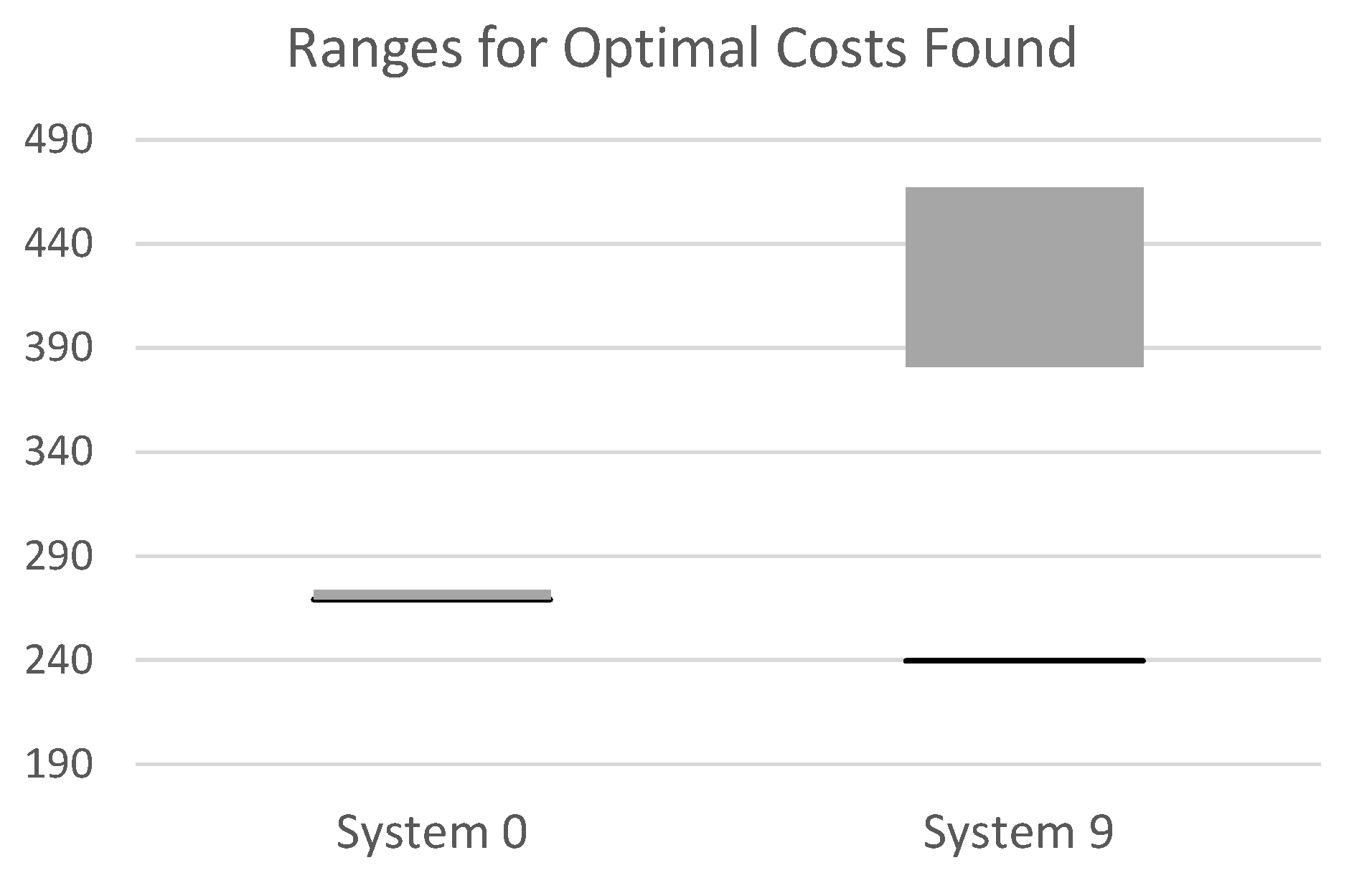
6. Results and Discussion

This section presents the results of mainly three sets of experiments. The first one compares our framework against approaches which use meta-heuristics for solving the CAP. In the second set of experiments, we compare our framework against SCALL. In the final set of experiments, we apply our framework in optimizing container allocations to heterogeneous devices in the contexts of Fog Computing and next generation wireless network planning.

In the first set of experiments, we apply our framework to solve the component allocation problems presented in [19]. These problems were collectively referred to as Systems 0 through 9. The models corresponding to the systems were obtained from the GitHub project on [36]. All of the models conform to the component allocation problem meta-model in [19]. The definition of these allocation problems was based on a realistic deployment problem of a vision-based software system on an autonomous underwater vehicle [16].

The allocation problems presented in [19] are of different sizes. For the allocation problems corresponding to Systems 0 to 4, the number of components is $C=11$ and the number of units is $U=4$. For Systems 5 and 6, the number of units is $U=8$ and the number of components is the same as that of Systems 0 to 4. For Systems 7 and 8, $U=16$ and $C=22$. System 9 represents the largest allocation problem and is composed of $U=32$ units and $C=30$ components. There are $M=3$ resources in all of the systems. The corresponding meta-model is the source meta-model for the model transformation example considered in Section 5.4.

Table 3. Optimal cost results for our framework, GA, and ACO.

	Our Framework	GA	ACO
System0	141.01	141.01	141.01
System1	176.62	176.62	176.62
System2	159.78	159.78	159.78
System3	186.16	186.16	186.16
System4	196.31	196.31	196.31
System5	108.10	122.09	108.27
System6	143.84	160.31	147.25
System7	202.28	285.57	273.38
System8	245.24	325.29	342.62
System9	263.38	452.82	452.66

compares the optimal cost results found by using our framework against those found by using implementations of two meta-heuristics for solving the component allocation problem: the first one is a genetic algorithm (GA), and the second is an ant colony optimization (ACO) algorithm. These implementations were presented in [19]. For the GA, the number of generations was set to 10,000, and for the ACO the number of iterations was 200. More details on the setup and parameters used for both meta-heuristics can be found in [19]. It is clear from the results that our framework returns optimal allocations that are the same or better (i.e., have less allocation cost) than those found by the GA and ACO meta-heuristics. This is especially true for large component allocation problems, such as those in Systems 7–9.

Table 4. The execution time results for our Framework, GA, and ACO (the unit is in seconds). SD stands for standard deviation.

	Our Framework		GA		ACO
	Mean	SD	Mean	SD	Mean	SD
System0	20.94	3.51	158.71	5.79	6949.38	190.36
System1	33.72	2.57	1092.26	88.62	7196.58	196.00
System2	35.25	4.10	1278.01	164.76	6820.97	201.67
System3	23.95	2.67	2962.68	307.75	6832.64	366.73
System4	21.72	2.33	7999.42	874.65	7137.78	364.83
System5	27.49	4.20	216.13	10.28	13,539.28	162.85
System6	27.93	2.70	213.58	16.48	13,740.06	279.69
System7	66.45	3.81	937.94	76.35	80,872.42	1598.87
System8	73.39	17.29	2133.85	240.11	84,292.41	2502.88
System9	165.63	14.09	1883.04	186.61	401,164.30	2986.01

shows the execution times comparing GA, ACO, and our framework. The reported statistical measures are based on samples of 10 runs for each system. The execution times are the elapsed times for executing the solvers, and they exclude the times for reading the input models and generating the output models. The experiments were carried out on a desktop computer with a 3.70 GHz dual-core processor and 8GB RAM. The results indicate that the execution times for the GA and ACO are several orders of magnitude larger than the execution times incurred by our framework. At the same time, the optimal allocations returned by our framework are better, as demonstrated in Table 3.

Figure 8 shows the Pareto fronts obtained by the multi-objective optimization of Systems 1 and 9. Without loss of generality and due to space constraints, we only include the results for these two systems. The scatter plots in the figure present visualizations of the objective space showing the non-dominated solutions in the Pareto fronts. For System 1, we implemented an exhaustive search algorithm to determine the Pareto front. The non-dominated solutions found by the exhaustive search method are colored in orange. On the other hand, the non-dominated solutions found by using our framework are marked with the character x. The Pareto fronts for System 1 are shown in Figure 8a. The figure shows that the set of non-dominated solutions found by our framework is a subset of the set of non-dominated solutions found by the exhaustive search method. Although our framework may not find all non-dominated solutions, it finds a good mix of non-dominated solutions that are distributed across the objective space of feasible solutions.

For System 9, the exhaustive search method becomes infeasible. Instead, we used Pymoo [37] to solve the multi-objective optimization problem. In particular, we applied the NSGA-II [38]. The algorithm follows the general outline of a genetic algorithm with a modified mating and survival selection. The non-dominated solutions found by Pymoo are colored in orange. The Pareto fronts for System 9 are shown in Figure 8b. The figure shows that some of the non-dominated solutions found by applying our framework are also found by using Pymoo. However, several of the non-dominated solutions found by applying our framework differ from those found by using Pymoo.

Considering the execution times for System 9, the 95% confidence interval (based on a sample of 10 runs) for the execution times was 3.4076 ± 0.052464 (the unit is in seconds) in the case of using Pymoo and 17.47997 ± 0.16062 in the case of using our framework. Note that for the NSGA-II, the population size was set to 100, and the number of generations was set to 100. The crossover rate was set to 0.90, and the mutation rate was set to 0.05.

In the second set of experiments, we apply our framework in solving allocation problems represented as models conforming to the meta-model of the SCALL tool [18]. This tool consists of two main parts: an editor that is used to create the models and a Python script, called PyAllocator, which is used to solve the allocation problem by employing a multi-objective heuristic allocation method. SCALL is implemented as an Eclipse plug-in and has been used in solving allocation problems in the research literature (for example, see the work of Švogor et al. [39]). Figure 9 shows the SCALL meta-model, which was adapted from [18]. The details of the meta-model can be found in [18]. We note that the meta-model does neither include elements for defining the weights nor the architectural constraints in a CAP.

To compare our framework against the SCALL tool, we instantiated two models conforming to the SCALL meta-model with the same parameters as Systems 0 and 9. Then, we used PyAllocator to solve the single-objective optimization problem. In the script, we defined the weights of the three resources by setting the elements of the trade-off vector $w_j$. There are no architectural constraints in the allocation problems. To apply our framework, we created a model transformation program to transform SCALL models into models conforming to the CAP meta-model. We used this transformation program to transform the models, which correspond to Systems 0 and 9.

Figure 10 shows optimal cost results obtained in 10 different runs. In the figure, the ranges for the approximated optimal costs (as found by SCALL) are represented as gray rectangles delimited by the minimum and maximum values in the different runs for each system. In addition, the figure shows the optimal cost for each system obtained using our framework as a solid black line. With regards to the execution times, for System 9, the 95% confidence interval for the execution times was 0.19447 ± 0.0022941 (the unit is in seconds) in the case of using the PyAllocator script and 0.16861 ± 0.0041780 in the case of using our framework.

Furthermore, we apply our proposed approach in order to extend and improve the previous works relying only on single-objective optimization in cases of conflicting goals. However, in such cases, conflicting aspects are present, such as infrastructure cost and energy consumption which should be kept as small as possible, while the performance has to be maximized, on the other side. Therefore, the adoption of multi-objective approach has the potential for improvement of the allocation outcome in these scenarios when there are several equivalent solutions with respect to cost minimization, but exhibit different performance or vice versa.

First, we considered the SMADA-Fog framework [40] which aims to find optimal container allocations to heterogeneous devices in the context of Fog Computing scenarios. In the original paper, the allocation problem is treated as a single-objective optimization problem aiming to minimize energy consumption or maximize execution speed under the constraints related to memory capacity, computing architecture (ARM/x86), and execution environment (Fog or Cloud). After the execution of the same experiments from [40], it was noticed that our approach was at least an order of magnitude faster regarding the execution time when it comes to the single-objective optimization case. Moreover, it was noticed that the speedup was more significant for larger models, reaching up to 2 orders of magnitude. On the other side, additional benefits were achieved using the proposed approach, as it enables multi-objective optimization of both energy consumption (minimization) and execution speed (maximization) at the same time. This way, it was possible to select more energy-efficient deployments for the same execution speed, while minimizing overall infrastructure maintenance costs. However, in the case of multi-objective optimization, the execution times were two orders of magnitude larger, reaching up to around 2.8 s in our experiments.

On the other side, similar findings are observed when it comes to the usage of our framework in the telecommunications domain for the optimal base station allocation at given smart city locations in the context of next-generation software-defined mobile networks [41]. The goal of the objective function is to minimize the deployment costs, while taking into account constraints related to fading-affected network performance and service demand. Apart from much faster execution in single-objective optimization mode in the case of large models (up to three orders of magnitude in case of more than 10 locations), the adoption of multi-objective optimization increased the QoS of the planned network deployment while reducing costs and energy consumption.

7. Conclusions and Future Work

In this paper, we have introduced a novel model-driven framework tackling the component allocation problem for both single- and multi-objective cases. The proposed solution was evaluated in the experiments based on several significant works in the area of software resource and computing infrastructure management. The results were compared to other solutions based on linear optimization tackling the CAP problem and other methods, such as GA and ACO, on the other side. Based on our experimental results, it can be concluded that our approach shows a faster execution time than GA (up to 3 orders of magnitude) and ACO (up to 5 orders of magnitude). Moreover, according to our results, it is also faster than several frameworks based on single-objective linear optimization, especially for larger models, up to two orders of magnitude. Furthermore, we extended several of the existing works with a multi-objective approach, achieving additional benefits, such as improved performance, while maintaining the infrastructure management costs and energy consumption as small as possible. Finally, we also include the optimal solution visualization workflow, which can help in decision-making in the case of multi-objective allocation.

To apply the proposed framework in solving a component allocation problem, the problem must be formulated as MOCAP (see Equations (1) and (2)). This requires the resource consumptions to have linear relationships with the possible allocations. Then, the modeler needs to create a model transformation into a model which conforms to the CAP meta-model. Although our framework may not be applicable to all allocation problems, we believe that the meta-model itself can be extended to accommodate a wider-variety of such problems. This would require extending the solver as well.

In future work, we would like to further exploit the results obtained as outcome of the optimization process for the purpose of code generation relying on domain-specific meta-models, such as the construction of virtual machine and container management commands in the case of software resource allocation or software-defined radio commands for a telecommunications case study. Additionally, the extension and adoption of the proposed approach in other domains is also planned, such as optimal resource planning during the COVID-19 pandemic. Finally, leveraging the synergy of optimization-based component allocation with predictions performed against the data collected during the system usage relevant to several allocation constraints can be considered in order to develop a new methodology for proactive resource planning.

References

1. Akdur, D.; Garousi, V.; Demirörs, O. A survey on modeling and model-driven engineering practices in the embedded software industry. J. Syst. Archit. 2018, 91, 62–82. [Google Scholar] [CrossRef] [Green Version]
2. Boussaïd, I.; Siarry, P.; Ahmed-Nacer, M. A survey on search-based model-driven engineering. Autom. Softw. Eng. 2017, 24, 233–294. [Google Scholar] [CrossRef]
3. Rodrigues da Silva, A. Model-driven engineering: A survey supported by the unified conceptual model. Comput. Lang. Syst. Struct. 2015, 43, 139–155. [Google Scholar] [CrossRef] [Green Version]
4. de Araújo Silva, E.; Valentin, E.; Carvalho, J.R.H.; da Silva Barreto, R. A survey of Model Driven Engineering in robotics. J. Comput. Lang. 2021, 62, 101021. [Google Scholar] [CrossRef]
5. Li, S.; Zhang, H.; Jia, Z.; Zhong, C.; Zhang, C.; Shan, Z.; Shen, J.; Babar, M.A. Understanding and addressing quality attributes of microservices architecture: A Systematic literature review. Inf. Softw. Technol. 2021, 131, 106449. [Google Scholar] [CrossRef]
6. Niknejad, N.; Ismail, W.; Ghani, I.; Nazari, B.; Bahari, M.; Hussin, A.R.B.C. Understanding Service-Oriented Architecture (SOA): A systematic literature review and directions for further investigation. Inf. Syst. 2020, 91, 101491. [Google Scholar] [CrossRef]
7. Tseng, F.H.; Jheng, Y.M.; Chou, L.D.; Chao, H.C.; Leung, V.C. Link-Aware Virtual Machine Placement for Cloud Services based on Service-Oriented Architecture. IEEE Trans. Cloud Comput. 2020, 8, 989–1002. [Google Scholar] [CrossRef]
8. Eclipse Modeling Framework (EMF). Available online: https://www.eclipse.org/modeling/emf/ (accessed on 15 November 2021).
9. Steinberg, D.; Budinsky, F.; Paternostro, M.; Merks, E. EMF: Eclipse Modeling Framework; Addison-Wesley Professional: Boston, MA, USA, 2008; Chapter 5. [Google Scholar]
10. OMG’s MetaObject Facility. Available online: http://www.omg.org/mof/ (accessed on 15 November 2021).
11. MDA. Available online: http://www.omg.org/mda/ (accessed on 15 November 2021).
12. ATL. Available online: https://www.eclipse.org/atl/ (accessed on 15 November 2021).
13. Jouault, F.; Allilaire, F.; Bézivin, J.; Kurtev, I. ATL: A model transformation tool. Sci. Comput. Program. 2008, 72, 31–39. [Google Scholar] [CrossRef]
14. Eclipse Modeling Project. Available online: https://eclipse.org/modeling/ (accessed on 15 November 2021).
15. QVT. Available online: http://www.omg.org/spec/QVT/ (accessed on 15 November 2021).
16. Švogor, I.; Crnković, I.; Vrček, N. An Extended Model for Multi-Criteria Software Component Allocation on a Heterogeneous Embedded Platform. J. Comput. Inf. Technol. 2013, 21, 211–222. [Google Scholar] [CrossRef]
17. Saaty, R.W. The Analytic Hierarchy Process—What it is and how it is used. Math. Model. 1987, 9, 161–176. [Google Scholar] [CrossRef] [Green Version]
18. Švogor, I.; Carlson, J. SCALL: Software Component Allocator for Heterogeneous Embedded Systems. In Proceedings of the European Conference on Software Architecture Workshops, New York, NY, USA, 7 September 2015; Association for Computing Machinery: New York, NY, USA, 2015; pp. 66:1–66:5. [Google Scholar]
19. Al-Azzoni, I.; Iqbal, S. Meta-Heuristics for Solving the Software Component Allocation Problem. IEEE Access 2020, 8, 153067–153076. [Google Scholar] [CrossRef]
20. Malek, S.; Medvidović, N.; Mikic-Rakic, M. An Extensible Framework for Improving a Distributed Software System’s Deployment Architecture. IEEE Trans. Softw. Eng. 2012, 38, 73–100. [Google Scholar] [CrossRef]
21. Koziolek, A.; Koziolek, H.; Reussner, R.H. PerOpteryx: Automated application of tactics in multi-objective software architecture optimization. In Proceedings of the International Conference on the Quality of Software Architectures and the International Symposium on Architecting Critical Systems, New York, NY, USA, 20–24 June 2011; pp. 33–42. [Google Scholar]
22. Deb, K.; Agrawal, S.; Pratap, A.; Meyarivan, T. A Fast Elitist Non-dominated Sorting Genetic Algorithm for Multi-objective Optimisation: NSGA-II. In Proceedings of the International Conference on Parallel Problem Solving from Nature, Leiden, The Netherlands, 5–9 September 2020; Springer: Berlin/Heidelberg, Germany, 2000; pp. 849–858. [Google Scholar] [CrossRef]
23. Becker, S.; Koziolek, H.; Reussner, R. The Palladio Component Model for Model-Driven Performance Prediction. J. Syst. Softw. 2009, 82, 3–22. [Google Scholar] [CrossRef]
24. Franks, G.; Omari, T.; Woodside, C.M.; Das, O.; Derisavi, S. Enhanced Modeling and Solution of Layered Queueing Networks. IEEE Trans. Softw. Eng. 2009, 35, 148–161. [Google Scholar] [CrossRef]
25. Koziolek, A.; Ardagna, D.; Mirandola, R. Hybrid multi-attribute QoS optimization in component based software systems. J. Syst. Softw. 2013, 86, 2542–2558. [Google Scholar] [CrossRef]
26. Aleti, A.; Björnander, S.; Grunske, L.; Meedeniya, I. ArcheOpterix: An extendable tool for architecture optimization of AADL models. In Proceedings of the Workshop on Model-Based Methodologies for Pervasive and Embedded Software, Vancouver, BC, Canada, 16 May 2009; IEEE Computer Society: Piscataway, NJ, USA, 2009; pp. 61–71. [Google Scholar] [CrossRef]
27. OSATE (Open Source AADL Tool Environment). Available online: https://osate.org (accessed on 15 November 2021).
28. Feiler, P.; Gluch, D.; Hudak, J. The Architecture Analysis and Design Language (AADL): An Introduction; Technical Report CMU/SEI-2006-TN-011; Software Engineering Institute, Carnegie Mellon University: Pittsburgh, PA, USA, 2006. [Google Scholar]
29. Aleti, A.; Grunske, L.; Meedeniya, I.; Moser, I. Let the Ants Deploy Your Software—An ACO Based Deployment Optimisation Strategy. In Proceedings of the International Conference on Automated Software Engineering, Auckland, New Zealand, 16–20 November 2009; IEEE Computer Society: Piscataway, NJ, USA, 2009; pp. 505–509. [Google Scholar] [CrossRef]
30. Li, R.; Etemaadi, R.; Emmerich, M.T.M.; Chaudron, M.R.V. An evolutionary multiobjective optimization approach to component-based software architecture design. In Proceedings of the Congress of Evolutionary Computation; IEEE: Piscataway, NJ, USA; pp. 432–439.
31. Wichmann, A.; Maschotta, R.; Bedini, F.; Zimmermann, A. Model-Driven Development of UML-Based Domain-Specific Languages for System Architecture Variants. In Proceedings of the International Systems Conference (SysCon), Orlando, FL, USA, 8–11 April 2019; IEEE: Piscataway, NJ, USA, 2019; pp. 1–8. [Google Scholar] [CrossRef]
32. Pohlmann, U.; Hüwe, M. Model-driven allocation engineering: Specifying and solving constraints based on the example of automotive systems. Autom. Softw. Eng. 2019, 26, 315–378. [Google Scholar] [CrossRef]
33. PyEcore. Available online: https://pyecore.readthedocs.io/en/latest/ (accessed on 15 November 2021).
34. ATL/User Guide. Available online: https://wiki.eclipse.org/ATL/User_Guide_-_The_ATL_Language#Helpers (accessed on 15 November 2021).
35. Das, I.; Dennis, J.E. Normal-Boundary Intersection: A New Method for Generating the Pareto Surface in Nonlinear Multicriteria Optimization Problems. SIAM J. Optim. 1998, 8, 631–657. [Google Scholar] [CrossRef] [Green Version]
36. Component Allocation Problem GitHub Project. Available online: https://github.com/ialazzon/ComponentAllocationProblem (accessed on 15 November 2021).
37. Blank, J.; Deb, K. Pymoo: Multi-Objective Optimization in Python. IEEE Access 2020, 8, 89497–89509. [Google Scholar] [CrossRef]
38. Deb, K.; Pratap, A.; Agarwal, S.; Meyarivan, T. A fast and elitist multiobjective genetic algorithm: NSGA-II. IEEE Trans. Evol. Comput. 2002, 6, 182–197. [Google Scholar] [CrossRef] [Green Version]
39. Švogor, I.; Crnković, I.; Vrček, N. An extensible framework for software configuration optimization on heterogeneous computing systems: Time and energy case study. Inf. Softw. Technol. 2019, 105, 30–42. [Google Scholar] [CrossRef]
40. Petrović, N.; Tosic, M. SMADA-Fog: Semantic model driven approach to deployment and adaptivity in fog computing. Simul. Model. Pract. Theory 2020, 101, 102033. [Google Scholar] [CrossRef]
41. Petrović, N.; Koničanin, S.; Milić, D.; Suljović, S.; Panić, S. GPU-enabled Framework for Modelling, Simulation and Planning of Mobile Networks in Smart Cities. In Proceedings of the Zooming Innovation in Consumer Technologies Conference, Novi Sad, Serbia, 26–27 May 2020; pp. 280–285. [Google Scholar] [CrossRef]
Figure 1. An example of a component allocation problem.
Algorithms 14 00354 g001
Figure 2. Overview of the objective space showing all eight solutions of the example.
Algorithms 14 00354 g002
Figure 3. Overview of the proposed framework for solving CAPs.
Algorithms 14 00354 g003
Figure 4. The CAP meta-model.
Algorithms 14 00354 g004
Figure 5. The solution set meta-model.
Algorithms 14 00354 g005
Figure 6. OCL assertions for the CAP meta-model.
Algorithms 14 00354 g006
Figure 7. Visualization of three solutions using petal diagrams.
Algorithms 14 00354 g007
Figure 8. Multi-objective optimization results for Systems 1 and 9. (a) Pareto fronts for System 1; (b) Pareto fronts for System 9.
Algorithms 14 00354 g008
Figure 9. The SCALL meta-model.
Algorithms 14 00354 g009
Figure 10. Optimal cost results for Systems 0 and 9.
Algorithms 14 00354 g010