Article

Optimized Weighted Nearest Neighbours Matching Algorithm for Control Group Selection

by
Szabolcs Szekér
and
Ágnes Vathy-Fogarassy
*,†
Department of Computer Science and Systems Technology, Faculty of Information Technology, University of Pannonia, 8200 Veszprém, Hungary
*
Author to whom correspondence should be addressed.
These authors contributed equally to this work.
Algorithms 2021, 14(12), 356; https://doi.org/10.3390/a14120356
Submission received: 31 October 2021 / Revised: 26 November 2021 / Accepted: 3 December 2021 / Published: 8 December 2021
(This article belongs to the Section Algorithms for Multidisciplinary Applications)

Abstract

:
An essential criterion for the proper implementation of case-control studies is selecting appropriate case and control groups. In this article, a new simulated annealing-based control group selection method is proposed, which solves the problem of selecting individuals in the control group as a distance optimization task. The proposed algorithm pairs the individuals in the n-dimensional feature space by minimizing the weighted distances between them. The weights of the dimensions are based on the odds ratios calculated from the logistic regression model fitted on the variables describing the probability of membership of the treated group. For finding the optimal pairing of the individuals, simulated annealing is utilized. The effectiveness of the newly proposed Weighted Nearest Neighbours Control Group Selection with Simulated Annealing (WNNSA) algorithm is presented by two Monte Carlo studies. Results show that the WNNSA method can outperform the widely applied greedy propensity score matching method in feature spaces where only a few covariates characterize individuals and the covariates can only take a few values.

Graphical Abstract

1. Introduction

Observational studies are widely applied data analysis methods mainly used in healthcare [1,2,3,4,5]. In these studies, the effect of a treatment, a risk factor, or other intervention is evaluated by performing a comparative analysis. The comparison is based on the analysis of the results of two groups, the treated and the untreated (control) groups, and the investigator has no control over the assignment of the subjects into the groups. Such analyses are carried out, for example, when the effectiveness of a drug for a particular disease is to be assessed (e.g., how effective a drug is at treating heart failure). In this case, the case group includes patients treated with the drug under investigation, while the control group includes patients who do not receive the drug. The comparison between the two groups can only be made adequately if the groups are similar in terms of the factors influencing the administration of the drug under study (e.g., severity of disease treated, comorbidities, drug sensitivity) and factors influencing the disease under study (in this example, age, lifestyle). For example, if only more severely ill or significantly older patients were selected in the control group, the result of the comparative analysis would be misleading. When the treated and the control groups are unbalanced to each other, the result of data analysis is often misleading. To get well-balanced treated and control groups, the bias of those covariates that simultaneously affect group assignment and the output variable of the study should be avoided. For balancing the two groups, different matching techniques were proposed. The simplest solution is based on stratified matching, but balancing score-based methods can also be used, and pairing of the treated and untreated individuals can also be performed in the n-dimensional space of the covariates.
Propensity score matching (PSM) [6] is the most widely applied balancing score-based matching method for selecting proper individuals into the control group. Despite the widespread use of the PSM method, it has received much criticism, as many articles point to the possible imbalance between the treated and control groups. When individuals are characterized by many covariates, the propensity scores of the individuals are diverse, and the PSM methods achieve a good performance. However, when only a few covariates are considered, and these covariates influence the selection of individuals with similar weighting factors, the PSM methods may result in a less balanced control group.
To solve the problem mentioned before, a nearest neighbour-based control group selection method (Weighted Nearest Neighbours Control Group Selection with Error Minimization, WNNEM) was proposed in our previous study [7]. However, the WNNEM method also has some limitations.
On the one hand, it cannot handle covariates negatively associated with the treatment assignment and, on the other hand, it uses local optimization to find the proper control group. In the current research, we aimed to eliminate these limitations. As a result, this article proposes a novel control group selection algorithm named Weighted Nearest Neighbours Control Group Selection with Simulated Annealing (WNNSA), which uses a global metaheuristic optimization method, namely simulated annealing for finding the best pairing of individuals. Furthermore, concerning the effect of the covariates, the proposed algorithm can also handle both positive and negative covariates. The new model can not only deal with variables related positively to the outcome variable (e.g., the risk of heart failure increases with age) but also variables negatively related to the outcome variable (e.g., taking an ACE inhibitor reduces the risk of heart failure). The efficiency of the newly proposed method will be presented by Monte Carlo simulations on two datasets. Results show that the new algorithm presented in this article outperforms the WNNEM method, the nearest neighbour matching, the Mahalanobis metric matching and the widely applied greedy PSM method in feature spaces where only a few covariates characterize individuals and the covariates can only take a few values.
The rest of the article is organized as follows. Section 2 provides a short overview of the control group selection task and presents the applied methods to solve the problem. In Section 3, the newly proposed WNNSA algorithm is presented in detail. Section 4 presents the methodology of the Monte Carlo simulations and the data used for the evaluations. Section 5 presents the results and, finally, Section 6 contains the main conclusions of the research.

2. Related Work

Control group selection aims to find such a group of individuals ( X U T ), which is similar to the individuals in the treated group ( X T ). The selection is generally performed by applying matching techniques so that proper individuals are selected from a set of possible candidates ( X C ). Although 1:1 and 1:N matching can also be performed, mostly 1:1 matching is applied. Matching should be performed on those baseline covariates ( f 1 , f 2 , , f n , n N ) that affect both the exposure of the group membership and the outcome variable of the study. As all individuals in X T , X C , and X U T are characterized by n features, they can be seen as n-dimensional objects in the n-dimensional vector space. Since the treated and control groups must be disjoint, it is a basic expectation that X T X C = .
In clinical research, the control group is mainly selected by propensity score matching. In this case, the pairing of individuals is performed in the one-dimensional space of the propensity scores. Propensity score (which is a balancing score) is the likelihood of the individuals being assigned to the treated group according to the baseline covariates, and it is usually calculated by a logistic regression fit [8,9]. In order to balance the bias of the treated and control groups, PSM selects those individuals into the control group who have similar propensity scores to the individuals in the treated group. The matching can be performed in different ways. The most widely applied PSM methods are nearest neighbour matching, radius matching, and inverse probability weighting [10,11,12]. The application of PSM has been the subject of numerous research, for example, its application was studied for subgroup analysis [13] and also for handling missing data [14].
Although different methods may produce control groups of different quality [15] (depending on the nature of the population used for selection), studies published in the literature most often only use the greedy PSM matching. Despite the popularity of the widely applied greedy k-nn-based PSM method, it has also got many criticisms [16,17,18,19,20,21,22]. All these articles pointed out that the PSM method in some cases and studies may result in a not well-balanced control group. For example, in [20] the authors highlighted that propensity score matching might increase imbalance even relative to the original data. The main limitation of the PSM methods is that they map the feature space into a single value (propensity score), and the matching of the individuals is performed in this compressed space. This can cause the problem of competing risks; this problem was also highlighted in [23].
However, the matching of the individuals can also be performed in the original feature space, and it is not necessary to compress the features into a single value. The simplest solution of this approach is stratified matching (SM) [24]. The condition for the successful application of stratified matching is that there should be enough candidates in each stratum to perform the pairing. The disadvantage of this method arises from the difficulty of handling continuous features.
The WNNEM method [7] also performs the matching in the original feature space of the individuals, but it utilizes the well-known k-nn principle for this purpose. This method can be seen as a hybrid combination of the PSM method and the nearest neighbour matching, as matching is performed based on the nearest neighbours, but the distances per dimension are weighted according to the relevance of the covariates (dimensions) calculated from a logistic regression fit. It was presented that the WNNEM method can select more balanced control groups than the greedy PSM method, especially in cases when individuals are characterized by only a few covariates and covariates can take only a few values [7].
Unfortunately, in many studies, control group selection is made by automatisms, and little attention is paid to the evaluation of the goodness of the control group. However, in the absence of this or in the case of bias in the control group, the results of the comparative analysis are questionable.
The similarity of case and control groups can be evaluated from different aspects. On the one hand, the distributions of the covariates have to be similar in the treated and control groups. On the other hand, having treated and control groups with similar distributions on the baseline variables does not mean that individuals are also similar to each other. Therefore, the similarity of the paired individuals should also be evaluated. This second criterion is also not sufficient as an independent criterion either because the distributions may contain bias in this case.
To measure the similarity of the distributions of the covariates, the standardized mean difference (SMD) [25] or goodness of fit tests can be used. For continuous variables, in the case of a normal distribution, the t-test [26], for general cases, the Kolmogorov–Smirnov [27,28] test can be calculated. For nominal data, the chi-squared test [29], for ordinal data, the Mann–Whitney U test [30] can be applied. The main drawback of these tests is that they evaluate the similarity of the treated group and the control group on only a single covariate. Calculating the Distribution Dissimilarity Index (DDI) [31] opens another aspect to the evaluations, as it calculates the similarity of the covariates based on the differences in the frequencies of the histograms of the covariates. In biomedical studies, the Hansen–Bowers test [32] is applied for more complex evaluations. This measure allows the evaluation of the imbalance of all covariates simultaneously.
As we mentioned before, the similarity of the distributions of the covariates does not mean that the matched individuals are also similar pairwise. The pairwise similarity of the matched objects can be evaluated by the Nearest Neighbour Index (NNI) and the Global Dissimilarity Index (GDI) [31]. The first measure only evaluates whether the paired individual is the closest individual from the candidate elements, while the second one considers the degree of the difference.

3. Weighted Nearest Neighbours Control Group Selection with Simulated Annealing (WNNSA)

The Weighted Nearest Neighbours Control Group Selection with Simulated Annealing algorithm proposed in this article is a distance-based method combined with simulated annealing (SA) [33]. The WNNSA method considers each subject as an n-dimensional data point in an n-dimensional space where each covariate ( f i , i = 1 , , n ) represents a unique dimension. Thus, control group selection can be interpreted as a distance minimization problem. To select a proper control group, those individuals have to be identified from the candidates that lie close to the individuals of the treated group. Because different covariates contribute differently to whether an individual is selected into the treated group, the closeness of the candidate individuals can not be calculated as a simple distance (e.g., Euclidean distance). For example, if the treated group includes individuals receiving a certain treatment, the application of the treatment may be affected differently by the age of the patient and the severity of the disease. Therefore, the WNNSA method takes the dimensions into account with different weights. The degree of influence is calculated from the regression coefficients of the logistic model fitted to the variable describing group membership. In this logistic regression model, the logit of the probability of belonging to the treated group of the individuals can be estimated as follows:
l o g i t ( p ) = l n p 1 p = b 0 + b 1 f 1 + b 2 f 2 + + b n f n ,
where p is the probability of belonging to the treated group and b i -s ( i = 1 , 2 , , n ) are the regression coefficients that describe the relative effects of the covariates ( f i , i = 1 , 2 , , n ).
The WNNSA method utilizes the odds ratio (OR) values of the fitted logistic regression model as weighting factors for the dimensions to compute the distances between the individuals. The weights for the features are calculated as:
w i = e x p b i O R i 1 1 e x p b i O R i < 1 ,
where w i yields the weight applied for the i-th dimension in the distance calculation. If O R i < 1 , then the covariate b i is negatively correlated to the assignment to the treated group, and if O R i 1 , the covariate is positively associated. The calculation of the weights of covariates with an OR value above 1 (positive association) is simple, and it can take any value above one as the weighting factor. In case of negative association, the weight of the covariate should be calculated as the reciprocal of the calculated OR value. This way, the weights of the negatively associated covariates can also take any value from ( 1 , ] , and it appropriately presents the weight of the covariate.
Having the extended calculation of the weighting factors, the distance matrix containing the pairwise distances of the individuals in the treated and candidate groups can be calculated by weighting the dimensions as follows:
d i s t ( X i , X j ) = l = 1 n w l d i j ( l ) ,
where d i j ( l ) denotes the normalized dissimilarity value of the X i X T and X j X C in the l-th dimension. Normalization of the distances along the dimensions is required to avoid the effect of the different ranges of the covariates [7].
As mentioned before, the WNNSA method considers control group selection as a distance minimization problem in the n-dimensional space. Distances between the individuals of the treated and control groups are calculated as weighted distances of the dimensions, and the aim is to match the control subjects to the treated subjects so that the sum of their distances is minimal. It is easy to see that in a simple case, when the neighbour closest to an individual in the treated group is chosen as the pair from the group of possible candidates, then the minimization problem is solved. The only problem arises when there are candidates closest to more than one individual of the treated group (conflicting candidates). The developed WNNSA algorithm presented aims to eliminate this problem.

Conflicting Candidates

The WNNSA algorithm solves the pairing of the proper individuals using metaheuristic population-based optimization. Each state in the search space represents a possible solution for the control group selection (a possible pairing of the individuals of the treated and control groups). The goal of the algorithm is to find the best pairing. To achieve this goal, the algorithm utilizes simulated annealing to select the best pairs for the treated individuals, and the goal is to minimize the sum of the pairwise distances of the paired individuals. The probability for selecting the candidate X j X C for the individual X i X T is calculated as:
p ( X i , X j ) = p t e m p ( X i , X j ) j p t e m p ( X i , X j ) ,
where
p t e m p ( X i , X j ) = 1 d i s t ( X i , X j ) t
and t is the temperature of the simulated annealing process.
The energy function (e) determining the fitness of the candidate solutions is given by Equation (6).
e = ( X i , X j ) M d i s t ( X i , X j ) ,
where M = { M 1 , M 2 , , M m } yields the pairing of the elements. In case of 1:1 matching, m = | X T | . For later use, denote M i 1 the first and M i 2 the second element from the i-th pair from M ( i = 1 , 2 , , m ).
In cases when individuals to be paired can be selected from many candidates, many possible pairings are conceivable. To reduce the runtime of the algorithm, the WNNSA algorithm looks for the optimal solution in a reduced search space. The applied heuristic constraints the search space in such a way that the individual of the treated group can only be paired to their k-nearest neighbours from the candidate set. Further neighbours are not considered for the pairing. Denote N N k ( X i , Y ) the k-closest neighbours of X i from the set Y. Using this notation, the k-size reduced environment for an individual X i X T is given by N N k ( X i , X C ) .
The detailed algorithm of the Weighted Nearest Neighbours Control Group Selection with Simulated Annealing method is presented in Algorithm 1. After the initialization of the variables (Step 1) and the normalization of the features (Step 2), the algorithm determines the sets of the k-nearest neighbours for all X i X T individuals (Steps 3 and 4). Steps 5 to 9 describe the simulated annealing optimization of the matching. In Step 5, the probabilities are calculated using the temperature parameter of the simulated annealing by Equation (4), and they are assigned to the elements. Step 8 describes the probability-based matching, while the detection of the conflicted candidates can be found in Step 9. The resolution of conflicts is made iteratively by repeating Steps 7 to 9. After finding a possible solution, the fitness value of the matching is calculated in Step 11. Following this, the actual matching is compared to the best result up to this point, and the better solution is saved as the best matching (Step 12). Finally, the temperature is reduced (Step 13). The simulated annealing process continues until the temperature reaches 0 (Step 14). The algorithm returns the control group with the lowest e ( t ) energy with the corresponding matching result (Step 15). For the sake of clarity, it should be noted that A c t u a l M a t c h i n g ( t ) denotes a transient set of matched pairs that the algorithm generates at temperature t. Furthermore, A c t u a l M a t c h i n g i ( t ) yields an element of this set, that is a specific matching of a treated element with a candidate element. Moreover, A c t u a l M a t c h i n g i 1 ( t ) denotes the first and A c t u a l M a t c h i n g i 2 ( t ) the second element of the matched pair of the i-th element from the set A c t u a l M a t c h i n g ( t ) . The first element comes from the treated group while the second one from the set of candidates to be paired as control individuals.
Algorithm 1: Weighted Nearest Neighbours Control Group Selection with Simulated Annealing (WNNSA).
Input:
X T : the set of the treated group; X C : the set of candidate individuals; k the size of the reduced environment; t m a x the starting temperature
Output:
X U T the selected control group; M the set of the matched pairs.
  • Initialize:    
        X U T =    
        M =    
        e b e s t =    
        t = t m a x
  • Normalize X T and X C collectively using feature scaling.
  • Calculate the distance matrix D for all pairs of X i X T and X j X C by Equation (3).
  • Determine N N k ( X i , X C ) based on the distance matrix D for all X i X T .
  • Determine p ( X i , X j ) for each X i X T and for each X j N N k ( X i , X C ) by Equation (4).
  • Set:    
        X u n p a i r e d ( t ) = X T    
        X U T ( t ) =    
        M ( t ) = .
  • Set A c t u a l M a t c h i n g s ( t ) =
  • For all X i X u n p a i r e d ( t )    
      Select an X j pair from N N k ( X i , X C ) for X i X u n p a i r e d ( t ) at random with probability p ( X i , X j ) .    
      Set A c t u a l M a t c h i n g s ( t ) = A c t u a l M a t c h i n g s ( t ) { ( X i , X j ) } .
  • For l = 1 , , | A c t u a l M a t c h i n g s ( t ) |    
      If A c t u a l M a t c h i n g s l 2 ( t ) is selected for only one X i X T
                 X u n p a i r e d ( t ) = X u n p a i r e d ( t ) { X i }
                 X U T ( t ) = X U T ( t ) { A c t u a l M a t c h i n g s l 2 ( t ) }
                 M ( t ) = M ( t ) { A c t u a l M a t c h i n g s l ( t ) }    
      End if
  • Repeat Steps 7 to 9, while X u n p a i r e d ( t ) .
  • Calculate the actual energy e ( t ) for the matching M ( t ) by Equation (6).
  • If e ( t ) < e b e s t    
       e b e s t = e ( t )    
       X U T = X U T ( t )    
       M = M ( t ) .
  • Set t = t 1 .
  • Repeat Steps 5 to 13 until t = 0 .
  • Return X U T and M.
As Algorithm 1 showed, the WNNSA method uses a reduced environment for selecting the elements of the control group. However, the application of a reduced environment introduces another problem. Below a given value of k, it is guaranteed that the algorithm will not result in a control group with the desired size. This stems from conflicts occurring during the selection process. For example, consider the following situation.
Let X 1 , X 2 , and X 3 be three individuals from the treated group. Let X 4 be the closest and X 5 the second-closest neighbour of X 1 and X 2 individuals among the candidate subjects. Furthermore, let X 5 be the first and X 4 the second nearest neighbour of X 3 . Moreover, let X 6 be the third nearest neighbour of X 1 , X 2 , and X 3 . Our aim is to select an equal-sized control group for the treated group. In this case, if we set k to 2, then the reduced environments for X 1 , X 2 , and X 3 contain only the individuals X 4 and X 5 . So, three individuals cannot be selected from the reduced environments; therefore, 1:1 matching can not be performed. This problem can also be extended to higher k values. For this reason, a method to determine the minimal k value is needed. A visual representation of the problem above can be seen in Figure 1.
The problem of unsolvable conflict described above can be solved mathematically. As mentioned before, N N k ( X i , Y ) denotes the k-closest neighbours of X i from the set Y. Additionally, denote X C k the aggregated reduced set of candidates for the k-sized environment as:
X C k = { X j | X j N N k ( X i , X C ) , X i X T } .
Furthermore, denote D e m ( X j ) those individuals from the treated group for which X j X C k is in their k-size reduced environment. D e m ( X j ) is called the demand set of X j , and it is calculated as:
D e m ( X j ) = { X i | X j N N k ( X i , X C ) } ,
where X i X T .
Let d i ( X j ) be the demand index for X j X C k quantifying those X i X T subjects which select X j as one of the k-nearest neighbours into the k-reduced environment. The demand index is calculated as:
d i ( X j ) = | D e m ( X j ) | k ,
where | D e m ( X j ) | yields the size of the demand set of X j .
Denote a s i ( X j ) the alternative selection index for X j , which quantifies the alternative selection options of X j for all X i D e m ( X j ) . Alternative selection means that the elements of the demand set of X j are paired to another candidate individual instead of X j . The alternative selection index for X j can be calculated as:
a s i ( X j ) = X i D e m ( X j ) m i n ( d i ( N N k ( X i , X C ) ) ) | D e m ( X j ) | .
Using these metrics, we can easily define the minimum size of the environment required for our pairing algorithm to succeed. If exists such an X j X C k that d i ( X j ) > 1 and a s i ( X j ) > 1 , there is an unsolvable conflict. In this case, the size of the environment (the value of k) have to be increased. The method to determine the minimum value of k is summarized in Algorithm 2.
Algorithm 2: Determination of the minimal size for the reduced environment for the WNNSA algorithm.
Input:
X T : the set of the treated group; X C : the set of candidate individuals
Output:
k m i n : the minimal size for the reduced environment.
  • Calculate the distance matrix D by Equation (3).
  • Set k = 1 .
  • Determine X C k by Equation (7).
  • For all X j X C k :    
      Calculate d i ( X j ) by Equation (9).    
      If d i ( X j ) > 1
           Calculate a s i ( X j ) by Equation (10).
           If a s i ( X j ) > 1
              k = k + 1
              Go Step 3
  • Return k.
After determining the size of the minimal reduced environment, the WNNSA algorithm can be executed. In order to perform a successful control group selection, the value of k must be initialized to at least the value determined by Algorithm 2. The higher the value of k is, the greater the degree of freedom the WNNSA algorithm has. However, it should also be taken into account that a too high value of k reduces the chances of the simulated annealing optimization to find the optimal pairing of the elements. Therefore, it is recommended to set the value of the k parameter first to the minimum required ( k m i n ), or a little higher. If the WNNSA algorithm does not finish in a short time (the conflict resolution problem is complex and the solution takes more time to find), it is recommended to iteratively increase the value of k by small increments until the algorithm stops. In our research, we found that k = k m i n 1.15 was the right choice in all cases, and the algorithm quickly found the right pairings of elements.

4. Study Design

To test the effectiveness of the proposed WNNSA method, several Monte Carlo simulations were performed. In this paper, two scenarios are presented. In Scenario I, a widely applied benchmark dataset [34] was used, which is commonly applied in theoretical PSM studies. As this dataset does not contain covariates that negatively affect the group assignment, we could only demonstrate the effectiveness of the simulated annealing optimization against the local optimization of the WNNEM method with this dataset. Additionally, results were also compared to the results of greedy PSM methods, the nearest neighbour matching, and the Mahalanobis metric matching. To present the effectiveness of the proposed method considering both negative and positive covariates, a novel, more complex, synthetic dataset was created in Scenario II. This scenario aims to present the advantage of the WNNSA method in a rare feature space containing only a few covariates with fewer values.
The rest of the section introduces the datasets and the methodology of the research in detail.

4.1. Dataset for Scenario I

The first dataset was generated according to [34]. In this scenario, individuals were characterized by ten binary variables arising from Bernoulli distributions ( x j B ( 0.5 ) , j = 1 , , 10 ). For the Monte Carlo simulations, 100 independent datasets were generated. All datasets contained 1000 individuals and approximately 25% of the sample were considered members of the treated group. The remaining individuals were considered as candidate subjects.
The logistic regression model to describe the probability for the treated group membership was formulated as described in [34]. The logistic model for the group assignment is presented by Equation (11).
logit ( p i , t r e a t ) = b 0 , t r e a t + b L x i 1 + b L x i 2 + b L x i 3 + b M x i 4 + b M x i 5 + b M x i 6 + b H x i 7 + b H x i 8 + b V H x i 9 + b V H x i 10 .
Weights ( b i , i = 1 , , 10 ) in Equation (11) denote a low (L), medium (M), high (H) and very high (VH) effect on group assignment. The applied weight coefficients were the following:
  • correction for binary: b 0 , t r e a t = 1.344090
  • low: b L = log ( 1.1 )
  • medium: b M = log ( 1.25 )
  • high: b H = log ( 1.5 )
  • very high: b V H = log ( 2.1 )

4.2. Dataset for Scenario II

The dataset used in Scenario II is a novel synthetic dataset generated for this study. This dataset contains fewer covariates than the previous one; therefore, it also better illustrates the problem of conflicting candidates. This dataset also contains covariates with negative and positive associations. Furthermore, it also contains nominal, ordinal and continuous variables.
In this dataset, every individual is characterized by two ordinal variables with Binomial distribution ( x j B ( 4 , 0.5 ) , j = 1 , , 2 ), four binary variables with Bernoulli distribution ( x j B ( 0.5 ) , j = 3 , , 6 ) and two continuous variables with Normal distribution ( x j N ( 2 , 0.6 ) , j = 7 , , 8 ). The weights b i are a mix of variables with negative and positive effect, described by Equation (12).
logit ( p i , t r e a t ) = b 0 , t r e a t b L x i 1 + b L x i 2 + b L x i 3 b M x i 4 + b M x i 5 + b M x i 6 + b H x i 7 b V H x i 8 ,
where b 0 , t r e a t = 1.344090 , b L = log ( 1.05 ) , b M = log ( 1.25 ) , b H = log ( 1.5 ) and b V H = log ( 1.9 ) . The dataset in each simulation contained 600 individuals and approximately 19% of the subjects were considered as the member of the treated group.

4.3. Methodology of the Evaluation

In our research, results of the WNNSA method were compared to the results of stratified matching (SM), nearest neighbour matching (NNM) [35], Mahalanobis metric matching (MMM) [36], two types of the PSM method and the WNNEM method.
In practical studies, the PSM method is generally applied with a restrictive condition. This constraint is controlled by setting the ‘caliper size’ parameter. Generally, the caliper size is set to 0.2 of the standard deviation of the logit of the propensity scores. This means that the control individuals can only be selected from a reduced environment of the treated elements. In the followings, this type of the PSM method is denoted as PSM_02. However, using this constraint, the control group selection method may also result in a control group that contains fewer individuals than the treated group. In case of the second version of the PSM method, for a fair evaluation, propensity score matching was executed with dynamic caliper size. It means that the size of the neighbourhood (aka the caliper size) of the treated individuals was determined dynamically such that in each case, an appropriately sized control group could be selected. In the following, this type of PSM method is denoted as PSM_DYN.
In the case of the WNNSA algorithm, the minimal size of the reduced k-size environment ( k m i n ) was calculated in accordance with Algorithm 2. To increase the search space and the freedom of the algorithm, the value of k was set to k = k m i n 1.15 in all scenarios.
As mentioned before, the effectiveness of the proposed methods was evaluated through Monte Carlo simulations. In each scenario, 100 independent datasets were generated with the given parameters. As WNNEM, SM, NNM and MMM are deterministic, they were only executed once on each generated dataset. In contrast, as PSM_02, PSM_DYN and WNNSA methods are not deterministic, they were executed ten times on each dataset. For these methods, the best result from the ten runs was considered for evaluation.
The quality of the selected control groups was evaluated from several perspectives. For distribution-based evaluation, SMD, t-test, chi-squared test, Hansen–Bowers test and Distribution Dissimilarity Index have been used. The pairwise similarities of the paired elements were evaluated by the Nearest Neighbour Index and the Global Dissimilarity Index.

5. Results

5.1. Results of the Scenario I

As was described before, the data-generating process in this scenario was identical to the one used in [34] to illustrate the efficiency of the proposed method on a widely used benchmark dataset.
The results of the algorithms were evaluated from different aspects. The individual balance values for the observed covariates are presented in Figure 2. When comparing balances, a method which could achieve the best results on all variables can not be selected. However, comparing the WNNEM and the WNNSA methods, it can be seen that the variable-wise balance is a little more diverse in the case of the WNNSA method than in the case of the WNNEM method. This result is not surprising since the WNNSA method does not always select the nearest neighbour from the candidates but balances the entire matching. To assess the balance of the groups by variables, we also calculated the SMD values for all covariates and all matching methods. The SMD values for all matching and covariates were less than 0.1, which confirms that according to the general evaluation principles, all results on all covariates can be seen as well-balanced.
The advantage of using the WNNSA method can be seen when looking at the similarity of control and case groups at the group level. To illustrate this, group-level quality indicators were also calculated. The results are presented in Table 1. Table 1 contains the minimal, average and maximal quality values of the control group selections performed on the generated 100 datasets. As DDI, NNI, and GDI metrics are distance measures, lower values mean more similar selected control groups. In contrast, in the case of the Hansen and Bowers test (HB), a higher value means higher similarity. The maximum possible value of the HB test is 1.
It can be seen in Table 1 that the SM method did not perform well on this dataset, and it could not select a full-sized control group. This fact can be inferred from the high values of the dissimilarity indices. Although the PSM methods performed well in distribution-based evaluations (HB, DDI), they under-performed by one order of magnitude in pairwise similarities (NNI, GDI) compared to the NNM, MMM, WNNEM and WNNSA methods. The NNM, MMM, WNNEM and WNNSA methods all performed well in the pairwise evaluations, but in the distribution-based evaluations, the WNNEM and WNNSA methods slightly outperformed the NNM and MMM methods. Comparing the WNNEM and WNNSA methods, we can see that the WNNEM method preferred selecting the nearest neighbours, while the WNNSA method aimed to achieve a global optimum. Across the four metrics, the WNNSA method scored best on three metrics and only on the NNI index (emphasizing nearest neighbour selection) scored slightly worse than algorithms that prefer nearest neighbour selection. However, this is understandable as WNNSA aims to achieve a global optimum, not a local optimum. Nevertheless, the difference is marginal.
As the Hansen and Bowers test is the most commonly used overall balance test, its values are also presented in detail for the 100 datasets in Figure 3. The smaller the interquartile range of the box is, the less different the control groups are, and the higher the box is placed, the more similar the selected control groups are to the case group. Figure 3 clearly shows that the WNNSA method performed the best. Apart from a few outlier values, it selected the most similar control groups with high confidence. If we look at the outliers, it also performed better than the other methods. For better visibility, Figure 3 does not include the results of the SM method as its outlier values were too low. For the sake of completeness, the results of SM are presented in text format: the first quartile (Q1) of data for SM is equal to 0.8092, the median of the data (Q2) is equal to 0.9235 and the third quartile of data (Q3) is equal to 0.9730.
Since the WNNSA method can be considered an improvement of the WNNEM method, it is worth comparing the results of these two methods in more detail. For the 100 datasets, the two methods gave the same results in 48 cases, the WNNEM method found more similar control groups in nine cases, while the WNNSA method outperformed the WNNEM method in 43 cases. In the nine cases where the WNNEM method produced better results than the WNNSA algorithm; the simulated annealing algorithm incorporated in the WNNSA method probably did not converge to the optimum. On the 100 datasets, the WNNEM method resulted in 0.9908 ± 0.0290 and the WNNSA algorithm in 0.9976 ± 0.0071 values on average for the Hansen and Bowers test.
Summarizing the results, we can see that when tested on the widely used benchmark dataset, the WNNSA method was able to more reliably select more similar control groups than the widely used PSM, the nearest neighbour methods or even the WNNEM method.

5.2. Results of the Scenario II

The dataset presented in Scenario I was based on a widely used, general benchmark dataset. As the proposed WNNSA method aims to improve the efficiency of the WNNEM method in a conflicted environment, such a kind of dataset was generated (see Section 4.2) for the second scenario. This dataset contains fewer descriptive features to better illustrate the problem arising from conflicting candidates. Additionally, it contains covariates with negative and positive associations and also nominal, ordinal and continuous variables. As this dataset contains negatively associated variables as well, the WNNEM method would not be able to run on it in its basic form. To perform a full evaluation, the WNNEM method was modified for this scenario to handle negative covariates. The dimension-wise weight calculation was extended to include O R i < 1 according to the Equation (2).
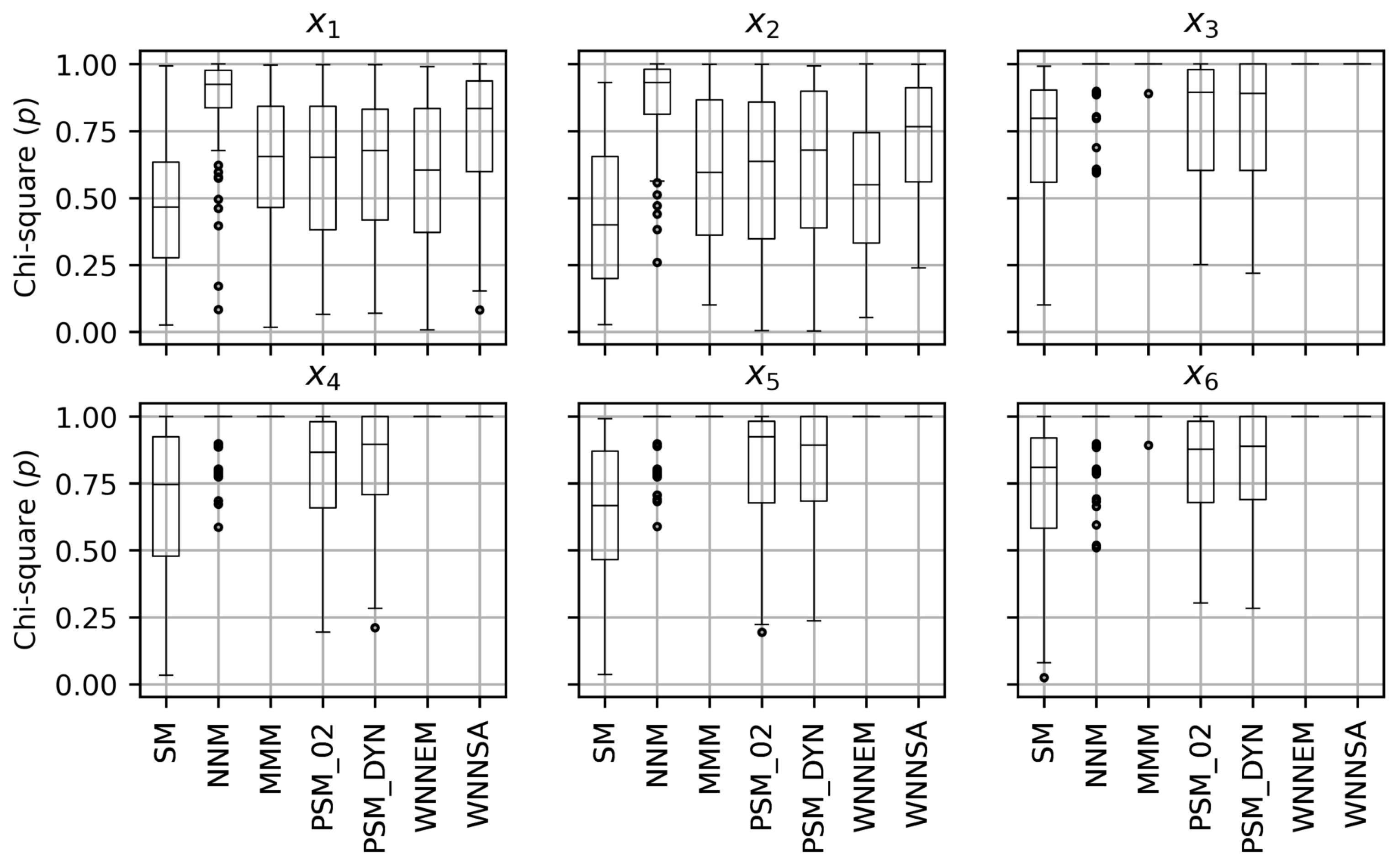
Figure 4 shows the individual balance values for ordinal and nominal variables. For the attributes x 1 and x 2 , the NNM method produced the most similar distributions. As these attributes had only minor influences on the value of the output variable, the WNNSA method placed less emphasis on their fitting. However, the second-best fit for these attributes was achieved by the the WNNSA method. Comparing the WNNSA method to the extended WNNEM method, the distribution of the balance in the case of x 1 and x 2 variables is better in the case of the WNNSA method. For attributes x 3 , x 4 , x 5 , x 6 , the WNNEM and WNNSA methods chose the same values for all paired individuals. This is partly because these are binary attributes at which the value-mismatch would result in a significant discrepancy; furthermore, some of them already had a medium impact on the outcome variable. That is, they had more effect on the distance calculations. The NNM method, which performed well on attributes x 1 and x 2 , did not always achieve an equivalent pairing for these attributes.
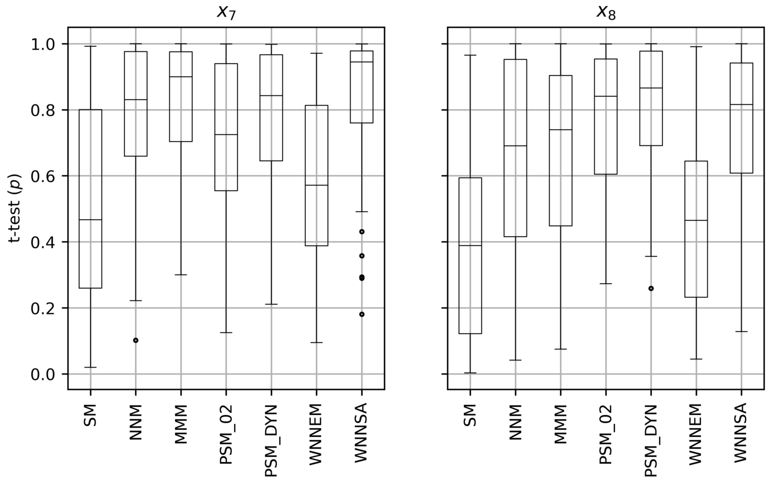
In the case of continuous variables (Figure 5), the extended WNNEM method gave the second worse results. The disadvantage of the WNNEM method in balancing continuous attributes is due to the local optimization and normalized distance computation. In the normalized distance calculation, the difference in the values of features with fewer values resulting in more significant differences in distance; however, a small difference between the values of the continuous attributes results in a more negligible difference between the two individuals. As the WNNEM method only selects from the two nearest neighbours, the WNNEM algorithm involuntarily favours value matching on variables with lower cardinality. The WNNSA method reduces this bias by working in a larger environment of the individuals and, thus, better balances the distribution of continuous feature values. In this way, the WNNSA method was able to improve the fit of the WNNEM method significantly, and on attribute x 7 it achieved the best fit. It also achieved a good result on attribute x 8 . Considering the results of Figure 4 and Figure 5 together, the WNNSA method achieved the best result for five out of eight attributes, the second-best match for two attributes, and the third best match for one attribute.
Table 2 shows the values of the group-level similarity and distance measures for Scenario II. The quality measures were calculated based on the result of the control group selections performed on the 100 datasets. It can be seen that the SM method yielded the worst results in most cases, analogously to Scenario I. Comparing the performance of the PSM-based methods with the nearest-neighbour based approaches, we can see that they perform similarly (PSM_DYN) or slightly worse (PSM_02) for the distribution-based indices (HB, DDI). However, they gave significantly worse results for the pairwise similarity indices (NNI, GDI). Comparing the results of the NNM, MMM, WNNEM and WNNSA methods, we can see that they produced similarly good results for all metrics, although the WNNSA method slightly outperformed the other methods. Comparing the WNNEM and WNNSA methods, the results are similar to Scenario I, but the differences between the two methods are more significant in this case.
The effectiveness of the WNNSA method is also clearly observable in Figure 6. The advantage of the WNNSA method is more pronounced in this conflicting environment since the interquartile range of the associated box plot is much smaller than the interquartile range of the box plot of the modified WNNEM method. At the same time, the top of both box diagrams is at a similar level. In addition, it can be seen, that although the extended WNNEM method performs slightly better than the PSM methods in the conflict environment, a more significant quality improvement occurs when the WNNSA method is used. Figure 6 also illustrates that, although the NNM and MMM methods also performed well on this dataset, the result of the WNNSA method outperforms them. The results of the SM method are only given in text format: Q 1 = 0.6105 , Q 2 = 0.7810 , and Q 3 = 0.9093 .
Comparing the WNNEM and WNNSA methods, it can be seen that the WNNSA method achieved significantly better results than the WNNEM method for the dataset presented in Scenario II. The main reason of this is that there are more conflict cases in this dataset, which the WNNSA method is more efficient in resolving. In 21 out of 100 datasets, the two methods achieved equally good results. In 6 cases, the WNNEM algorithm resulted in more similar control groups than the WNNSA algorithm. However, the WNNSA algorithm outperformed the WNNEM algorithm on 73 datasets. The WNNEM method resulted in 0.9690 ± 0.0479 and the WNNSA algorithm in 0.9917 ± 0.0236 values on average for the Hansen and Bowers test.

6. Conclusions

Observational studies are widely applied data analysis methods in life sciences, in which the quality of the results is mainly determined by the control group selection process. The more similar the selected control group and the case group are to each other, the more reliable the result of the analysis is.
In this paper, an optimized k-nearest neighbours-based control group selection method, called Weighted Nearest Neighbours Control Group Selection with Simulated Annealing (WNNSA), was proposed. The WNNSA method applies simulated annealing to find the best pairing of treated individuals and candidates for selecting for the control group. The optimization is performed in the original feature space of the objects and not in the compressed space of the balancing scores, as the widely applied PSM method does. Furthermore, in contrast to the WNNEM method, optimization is performed on a global level.
The efficiency of the WNNSA method was presented by Monte Carlo simulations. Simulation results confirmed that the WNNSA method could outperform the stratified matching-based control group selection method, the nearest neighbour matching, the Mahalanobis metric matching, the WNNEM method, and the widely applied greedy propensity score matching method in feature spaces where only a few covariates characterize individuals, and the covariates can only take a few values. In this restricted feature space, numerous conflicted situations may arise in the selection of similar individuals, which can be effectively handled by the proposed WNNSA algorithm.

Author Contributions

Conceptualization, S.S. and Á.V.-F.; methodology, S.S. and Á.V.-F.; software, S.S.; validation, S.S. and Á.V.-F.; formal analysis, S.S. and Á.V.-F.; investigation, S.S. and Á.V.-F.; data curation, S.S. and Á.V.-F.; writing—original draft preparation, S.S. and Á.V.-F.; writing—review and editing, S.S. and Á.V.-F.; visualization, S.S. and Á.V.-F.; supervision, Á.V.-F.; project administration, S.S. and Á.V.-F.; funding acquisition, Á.V.-F. All authors have read and agreed to the published version of the manuscript.

Funding

This research received no external funding.

Institutional Review Board Statement

Not applicable.

Informed Consent Statement

Not applicable.

Data Availability Statement

Data supporting reported results can be found at https://github.com/vathyfogarassy/WNNSA (accessed on 30 October 2021).

Acknowledgments

We acknowledge the professional support of GINOP-2.2.1-15-2016-00019 “Development of intelligent, process-based decision support system for cardiologists”.

Conflicts of Interest

The authors declare no conflict of interest.

Abbreviations

The following abbreviations are used in this manuscript:
DDIDistribution Dissimilarity Index
GDIGlobal Dissimilarity Index
HBHansen and Bowers test
MMMMahalanobis metric matching
NNNearest neighbour
NNINearest Neighbour Index
NNMNearest neighbour matching
OROdds ratio
PSMPropensity Score Matching
SASimulated annealing
SMStratified matching
SMDStandardized mean difference
WNNEMWeighted Nearest Neighbours Control Group Selection with Error Minimization
WNNSAWeighted Nearest Neighbours Control Group Selection with Simulated Annealing

References

  1. Sirois, C. Case-Control Studies. In Encyclopedia of Pharmacy Practice and Clinical Pharmacy; Babar, Z.U.D., Ed.; Elsevier: Oxford, UK, 2019; pp. 356–366. [Google Scholar] [CrossRef]
  2. Li, L.; Donnell, E.T. Incorporating Bayesian methods into the propensity score matching framework: A no-treatment effect safety analysis. Accid. Anal. Prev. 2020, 145, 105691. [Google Scholar] [CrossRef]
  3. Li, Q.; Lin, J.; Chi, A.; Davies, S. Practical considerations of utilizing propensity score methods in clinical development using real-world and historical data. Contemp. Clin. Trials 2020, 97, 106123. [Google Scholar] [CrossRef]
  4. Fang, Y.; He, W.; Wang, H.; Wu, M. Key considerations in the design of real-world studies. Contemp. Clin. Trials 2020, 96, 106091. [Google Scholar] [CrossRef] [PubMed]
  5. Kondo, Y.; Noda, T.; Sato, Y.; Ueda, M.; Nitta, T.; Aizawa, Y.; Ohe, T.; Kurita, T. Comparison of 2-year Outcomes between Primary and Secondary Prophylactic Use of Defibrillators in Patients with Coronary Artery Disease: A Prospective Propensity Score-Matched Analysis from the Nippon Storm Study. Heart Rhythm O2 2021, 2, 5–11. [Google Scholar] [CrossRef]
  6. Rosenbaum, P.R.; Rubin, D.B. The central role of the propensity score in observational studies for causal effects. Biometrika 1983, 70, 41–55. [Google Scholar] [CrossRef]
  7. Szekér, S.; Vathy-Fogarassy, Á. Weighted nearest neighbours-based control group selection method for observational studies. PLoS ONE 2020, 15, e0236531. [Google Scholar] [CrossRef]
  8. Wright, R.E. Logistic Regression; American Psychological Association: Washington, DC, USA, 1995. [Google Scholar]
  9. Rudaś, K.; Jaroszewicz, S. Linear regression for uplift modeling. Data Min. Knowl. Discov. 2018, 32, 1275–1305. [Google Scholar] [CrossRef] [Green Version]
  10. Baser, O. Too much ado about propensity score models? Comparing methods of propensity score matching. Value Health 2006, 9, 377–385. [Google Scholar] [CrossRef] [Green Version]
  11. Caliendo, M.; Kopeinig, S. Some Practical Guidance for the Implementation of Propensity Score Matching. J. Econ. Surv. 2008, 22, 31–72. [Google Scholar] [CrossRef] [Green Version]
  12. Austin, P.C. An introduction to propensity score methods for reducing the effects of confounding in observational studies. Multivar. Behav. Res. 2011, 46, 399–424. [Google Scholar] [CrossRef] [Green Version]
  13. Zhang, Y.; Schnell, P.; Song, C.; Huang, B.; Lu, B. Subgroup causal effect identification and estimation via matching tree. Comput. Stat. Data Anal. 2021, 159, 107188. [Google Scholar] [CrossRef]
  14. Shi, J.; Qin, G.; Zhu, H.; Zhu, Z. Communication-efficient distributed M-estimation with missing data. Comput. Stat. Data Anal. 2021, 16, 107251. [Google Scholar] [CrossRef]
  15. Tousi, S.S.; Tabesh, H.; Saki, A.; Tagipour, A.; Tajfard, M. Comparison of Nearest Neighbor and Caliper Algorithms in Outcome Propensity Score Matching to Study the Relationship between Type 2 Diabetes and Coronary Artery Disease. J. Biostat. Epidemiol. 2021, 7, 251–262. [Google Scholar] [CrossRef]
  16. Austin, P.C. A critical appraisal of propensity-score matching in the medical literature between 1996 and 2003. Stat. Med. 2008, 27, 2037–2049. [Google Scholar] [CrossRef] [PubMed]
  17. Pell, G.S.; Briellmann, R.S.; Chan, C.H.P.; Pardoe, H.; Abbott, D.F.; Jackson, G.D. Selection of the control group for VBM analysis: Influence of covariates, matching and sample size. Neuroimage 2008, 41, 1324–1335. [Google Scholar] [CrossRef]
  18. Biondi-Zoccai, G.; Romagnoli, E.; Agostoni, P.; Capodanno, D.; Castagno, D.; D’Ascenzo, F.; Sangiorgi, G.; Modena, M.G. Are propensity scores really superior to standard multivariable analysis? Contemp. Clin. Trials 2011, 32, 731–740. [Google Scholar] [CrossRef] [Green Version]
  19. Mansournia, M.A.; Jewell, N.P.; Greenland, S. Case–control matching: Effects, misconceptions, and recommendations. Eur. J. Epidemiol. 2018, 33, 5–14. [Google Scholar] [CrossRef] [PubMed]
  20. King, G.; Nielsen, R. Why propensity scores should not be used for matching. Political Anal. 2019, 27, 435–454. [Google Scholar] [CrossRef] [Green Version]
  21. Moser, P. Out of Control? Managing Baseline Variability in Experimental Studies with Control Groups. Handb. Exp. Pharmacol. 2019, 257, 101–117. [Google Scholar] [CrossRef] [Green Version]
  22. Wan, F. Matched or unmatched analyses with propensity-score-matched data? Stat. Med. 2019, 38, 289–300. [Google Scholar] [CrossRef]
  23. He, Y.; Kim, S.; Kim, M.O.; Saber, W.; Ahn, K.W. Optimal treatment regimes for competing risk data using doubly robust outcome weighted learning with bi-level variable selection. Comput. Stat. Data Anal. 2021, 158, 107167. [Google Scholar] [CrossRef]
  24. Anderson, D.W.; Kish, L.; Cornell, R.G. On stratification, grouping and matching. Scand. J. Stat. 1980, 7, 61–66. [Google Scholar]
  25. Austin, P.C. Balance diagnostics for comparing the distribution of baseline covariates between treatment groups in propensity-score matched samples. Stat. Med. 2009, 28, 3083–3107. [Google Scholar] [CrossRef] [Green Version]
  26. Gosset, W.S. The probable error of a mean. Biometrika 1908, 1–25. [Google Scholar] [CrossRef]
  27. Kolmogorov, A. Sulla determinazione empirica di una lgge di distribuzione. Inst. Ital. Attuari Giorn. 1933, 4, 83–91. [Google Scholar]
  28. Smirnov, N. Table for estimating the goodness of fit of empirical distributions. Ann. Math. Stat. 1948, 19, 279–281. [Google Scholar] [CrossRef]
  29. Pearson, K.X. On the criterion that a given system of deviations from the probable in the case of a correlated system of variables is such that it can be reasonably supposed to have arisen from random sampling. Lond. Edinb. Dublin Philos. Mag. J. Sci. 1900, 50, 157–175. [Google Scholar] [CrossRef] [Green Version]
  30. MacFarland, T.W.; Yates, J.M. Mann–Whitney U test. In Introduction to Nonparametric Statistics for the Biological Sciences Using R; Springer: Berlin/Heidelberg, Germany, 2016; pp. 103–132. [Google Scholar]
  31. Szekér, S.; Vathy-Fogarassy, Á. How Can the Similarity of the Case and Control Groups be Measured in Case-Control Studies? In Proceedings of the 2019 IEEE International Work Conference on Bioinspired Intelligence (IWOBI), Budapest, Hungary, 3–5 July 2019; pp. 33–40. [Google Scholar] [CrossRef]
  32. Bowers, J.; Fredrickson, M.; Hansen, B. RItools: Randomization inference tools. R Package Version 0.1-11. 2010. [Google Scholar]
  33. Van Laarhoven, P.J.; Aarts, E.H. Simulated Annealing: Theory and Applications; Springer: Berlin/Heidelberg, Germany, 1987. [Google Scholar]
  34. Austin, P.C. Comparing paired vs non-paired statistical methods of analyses when making inferences about absolute risk reductions in propensity-score matched samples. Stat. Med. 2011, 30, 1292–1301. [Google Scholar] [CrossRef] [Green Version]
  35. Rubin, D.B. Matching to remove bias in observational studies. Biometrics 1973, 29, 159–183. [Google Scholar] [CrossRef]
  36. Rubin, D.B. Bias reduction using Mahalanobis-metric matching. Biometrics 1980, 36, 293–298. [Google Scholar] [CrossRef]
Figure 1. Demonstration of conflicting pairs in a reduced environment X 1 , X 2 and X 3 are three individuals from the treated group and X 4 , X 5 , and X 6 are three individuals from the candidate group. In the case of a k = 2 reduced environment, 1:1 matching cannot be performed; while in the case of a k = 3 reduced environment, conflicts can be resolved.
Algorithms 14 00356 g001
Figure 2. Similarities of the case and control groups on each attribute in Scenario I. Distributions of the Chi-square p-values were calculated separately for each covariate.
Algorithms 14 00356 g002
Figure 3. Results of the Hansen and Bowers test in Scenario I. Comparison of the p-values of the Hansen and Bowers test in case of the nearest neighbour matching (NNM), Mahalanobis metric matching (MMM), two types of PSM methods (PSM_02, PSM_DYN), the WNNEM method and the WNNSA method for the 100 datasets in Scenario I.
Algorithms 14 00356 g003
Figure 4. Similarities of the case and control groups on ordinal and binary attributes in Scenario II. Distributions of the Chi-square p-values calculated for ordinal ( x 1 , x 2 ) and binary ( x 3 , x 4 , x 5 , x 6 ) covariates separately, based on all simulations in Scenario II.
Algorithms 14 00356 g004
Figure 5. Distribution of continuous covariates in Scenario II. Distribution of the t-test p-values calculated for each covariate separately based on all simulations in Scenario II.
Algorithms 14 00356 g005
Figure 6. Results of Hansen and Bowers tests in Scenario II. Comparison of the p-values of the Hansen and Bowers test in case of the nearest neighbour matching (NNM), Mahalanobis metric matching (MMM), two types of PSM methods (PSM_02, PSM_DYN), the WNNEM method, and the WNNSA method for the 100 datasets in Scenario II.
Algorithms 14 00356 g006
Table 1. Measures for evaluating the group-level similarities of case and control groups in Scenario I. HB(p) denotes the p-value of the Hansen and Bowers test, DDI(d) represents the dissimilarity value of the Distribution Dissimilarity Index, NNI(d) stands for the dissimilarity value of the Nearest Neighbour Index, and GDI(d) is the dissimilarity value of the Global Dissimilarity Index. In the case of HB(p), the higher value is better, while in the case of DDI(d), NNI(d) and GDI(d), the lower value is better.
NNMMMMSM
min avg max min avg max min avg max
HB(p)0.5830.9761.0000.3470.9601.0000.5120.8731.000
DDI(d)0.0060.0150.0350.0040.0150.0300.5040.5740.631
NNI(d)0.0540.0650.0750.0570.0660.0780.5040.5740.631
GDI(d)0.0620.0750.0950.0590.0760.0970.5040.5740.631
PSM_02PSM_DYNWNNEMWNNSA
min avg max min avg max min avg max min avg max
HB(p)0.8130.9781.0000.9040.9931.0000.7400.9911.0000.9550.9981.000
DDI(d)0.0210.0610.1160.0060.0140.0230.0060.0120.0220.0050.0110.021
NNI(d)0.1940.3160.3740.1900.2780.3250.0520.0600.0700.0560.0700.080
GDI(d)0.2140.3480.4160.2120.3130.3670.0520.0610.0770.0620.0730.097
Table 2. Measures for evaluating the group-level similarities of case and control groups in Scenario II. HB(p) denotes the p-value of the Hansen and Bowers test, DDI(d) represents the dissimilarity value of the Distribution Dissimilarity Index, NNI(d) stands for the dissimilarity value of the Nearest Neighbour Index, and GDI(d) is the dissimilarity value of the Global Dissimilarity Index. In the case of HB(p), the higher value is better, while in the case of DDI(d), NNI(d) and GDI(d), the lower value is better.
NNMMMMSM
min avg max min avg max min avg max
HB(p)0.4320.9681.0000.6860.9741.0000.1400.7240.995
DDI(d)0.0340.0610.0930.0350.0580.0840.6170.7100.800
NNI(d)0.3000.3250.3620.2890.3050.3310.7180.7890.858
GDI(d)0.0430.0580.0810.0540.0710.1070.6370.7280.815
PSM_02PSM_DYNWNNEMWNNSA
min avg max min avg max min avg max min avg max
HB(p)0.5230.9411.0000.7290.9601.0000.7690.9691.0000.8150.9911.000
DDI(d)0.0620.1020.1620.0500.0720.1020.0320.0560.0780.0340.0520.071
NNI(d)0.5910.6610.7050.5280.6400.6780.2850.3030.3210.3000.3180.335
GDI(d)0.3140.4110.4630.2790.3760.4460.0350.0460.0570.0430.0560.069
Publisher’s Note: MDPI stays neutral with regard to jurisdictional claims in published maps and institutional affiliations.