Towards Interactive Analytics over RDF Graphs

Abstract

The continuous accumulation of multi-dimensional data and the development of Semantic Web and Linked Data published in the Resource Description Framework (RDF) bring new requirements for data analytics tools. Such tools should take into account the special features of RDF graphs, exploit the semantics of RDF and support flexible aggregate queries. In this paper, we present an approach for applying analytics to RDF data based on a high-level functional query language, called HIFUN. According to that language, each analytical query is considered to be a well-formed expression of a functional algebra and its definition is independent of the nature and structure of the data. In this paper, we investigate how HIFUN can be used for easing the formulation of analytic queries over RDF data. We detail the applicability of HIFUN over RDF, as well as the transformations of data that may be required, we introduce the translation rules of HIFUN queries to SPARQL and we describe a first implementation of the proposed model.

1. Introduction

The amount of data available on the Web today is increasing rapidly due to successful initiatives, such as the Linked Open Data movement (http://lod-cloud.net/). More and more data sources are being exported or produced using the Resource Description Framework (https://www.w3.org/RDF/) (or RDF, for short) standardized by the W3C. There are thousands of published RDF datasets (see [1] for a recent survey), including cross-domain knowledge bases (KBs) (e.g., DBpedia [2] and Wikidata [3]), domain specific repositories (e.g., DrugBank [4], GRSF [5], ORKG [6], WarSampo [7], and recently COVID-19 related datasets [8,9,10] as well as Markup data through schema.org.

Figure 1 shows the general picture of access services over RDF. Apart from Structured Query Languages, we have Keyword Search systems over RDF (like [11]) that allow users to search for information using the familiar method they use for Web searching. We can also identify the category Interactive Information Access that refers to access methods that are beyond the simple “query-and-response“ interaction, i.e., methods that offer more interaction options to the user and also exploit the interaction session. In this category, there are methods for RDF Browsing, methods for Faceted Search over RDF [12], as well as methods for Assistive (SPARQL) Query Building (e.g., [13]). Our work falls in this category, specifically we aim at providing an interactive method for analytics over RDF. Finally, in the category natural language interfaces there are methods for question answering, dialogue systems, and conversational interfaces.

As regards structured query languages, RDF data are mainly queried through structured query languages, i.e., SPARQL (https://www.w3.org/TR/rdf-sparql-query/), which is the standard query language for RDF data. SPARQL supports complex querying using regular path expressions, grouping, aggregation, etc., but the application of analytics to RDF data and especially to large RDF graphs is not so straightforward. The structure of such graphs tends to be complex due to several factors: (i) different resources may have different sets of properties, (ii) properties can be multi-valued (i.e., there can be triples where the subject and predicate are the same but the objects are different) and (iii) resources may or may not have types. On the other hand, the regular methods of analytics are not capable of analyzing RDF graphs effectively, as they (i) focus on relational data, (ii) can only work with a single homogeneous data set, (iii) neither support multiple central concepts, nor RDF semantics, (iv) do not offer flexible choices of dimension, measure, and aggregation and (v) demand deep knowledge of specific query languages depending on data’s structure.

In view of the above challenges, there is a need for a simple conceptual model able to guide data analysis over one or more linked data sets that demands no programming skill. Motivated from this need, we are investigating an approach based on a high-level query language, called HIFUN [14], for applying analytics to RDF graphs. We study how that language can be applied to RDF data by clarifying how the concept of analysis context can be defined, what kind of transformations are required and how HIFUN queries are translated to SPARQL. Please note that with the translation approach that we focus on, we can apply analytics to RDF sources, without having to transform the RDF data to relational ones, nor to copy them.

The idea was first introduced in [15]. The current paper is an extended and enriched version of that work presenting (a) a more complete related work, (b) a detailed analysis of the applicability of HIFUN over RDF data, (c) the detailed algorithm for translating HIFUN queries over RDF data, (d) the first implementation of an algorithm that makes that translation.

The remainder of the paper is organized as follows: Section 2 discusses the requirements for analyzing RDF data and the research that has been conducted in that area. Section 3 introduces the related background knowledge. Section 4 focuses on how HIFUN can be used as an interface to RDF data. Section 5 investigates whether HIFUN can be applied to RDF data. Section 6 details the translation algorithm, Section 7 discusses interactivity issues, and finally Section 8 concludes this paper and suggests directions for future research.

2. Requirements and Related Work

In this section, we describe the requirements of analyzing semantic warehouses and we survey the related work that has been conducted in the area of RDF analytics.

2.1. Requirements

In decision-support systems, to extract useful information from the data of an application, it is necessary to analyze large amounts of data accumulated over time—typically over a period of several months. This data is usually stored in a so-called “data warehouse” and analysed along various dimensions and at various levels in each dimension [16]. The end users of such warehouses are mainly analysts and decision-makers, who invariably ask for data aggregations (e.g., total sales by branch).

During last decade the development of Semantic Web data has led to the emergence of semantic warehouses; specific-domain warehouses [17,18] or general-purpose knowledge bases (e.g., DBpedia and WikiData (https://www.wikidata.org)). Thus, it would be useful if the data of these warehouses could be analyzed to extract valuable information (e.g., identify patterns, predict values, discover data correlations), check the quality of semantic integration activities (e.g., for measuring the commonalities between several data sets [19,20]) or monitor the content and the quality of them (e.g., by evaluating the completeness or the representativeness of its data etc.).

However, the analysis of such warehouses introduces several challenges [21]. The data heterogeneity, its lack of a strict structure, its rich semantics and the possibility of incomplete data sources significantly complicates their analysis. For example, although one can reasonably expect to find information about a particular concept, they cannot always find specific information for all the instances of it (e.g., the opening hours or closing days of all branch stores). Moreover, data warehouses follow a star schema and thus, the facts can be analyzed based on certain dimensions and measures, the choice of which is made at the data warehouse design time (e.g., if “branch” and “product” have been defined as dimensions, then aggregations over them are not allowed; one cannot find “the number of branches established in 2020, since “branch” is a dimension and relational data cubes do not allow aggregating over dimensions). In addition, different concepts (e.g., “branches”, “products”, “people”) can be analyzed, only if each of them is modeled by a different schema and stored in a distinct data warehouse. Finally, even though such warehouses host data published along with a schema (which can facilitate the understanding of data), the structure of it tends to be complex. Please also note that the end-users, who are usually non-specialists, are unable to read the schema and formulate the queries necessary for their data analysis. Thus, it would be useful if apart from native RDF data, one could analyze and deduce further knowledge (inference) from RDF schemas, too (e.g., ask for all the relationships linking products to other entities).

Therefore, there is a need to be able to apply analytics to any kind of RDF graph—not only to multidimensional data expressed in RDF, but also to domain-specific or general-purpose semantic data; a way that will be applicable to several RDF data sets, as well as to any data source. In general, we need an analytical tool that will allow the user to select the desired data set(s) or desired parts thereof, define the features (s)he is interested in at the query time, formulate an analytic query without having any programming background knowledge and will display the results in the form of tables, plots or any other kind of visualization for intuitive exploration.

2.2. Related Work

Statistical data is published as linked data in order to be combined with data sets that are published in disparate sources on the Web. Such data should have been modeled as data cubes describing data in a multi-dimensional fashion. To this end, the RDF data cube vocabulary (https://www.w3.org/TR/vocab-data-cube/) (QB) is employed. This vocabulary provides a means to publish such data on the web using the W3C RDF standard. It consists of three main components: (i) the measures, which are the observed values of primary interest, (ii) the dimensions, which are the value keys that identify the measure and (iii) the attributes, which are the metadata. However, even though that vocabulary can be used for structuring and publishing multi-dimensional data, it cannot be used for applying analytics over it. In view of this limitation, several approaches were proposed.

These approaches can be divided into two major groups: (i) those assuming that the multidimensional data (MD) i.e., data related to more than two dimensions, has already been represented in the RDF format and (ii) those that do not. Our approach, as well as the works in [22,23,24] are related to the first group. On the other hand, the work in [25] considers that the multidimensional data has been stored as non-RDF data sets. In particular, it declares that the data cubes are retrieved from a relational database with SQL queries and then get triplicated.

The representation of MD data in RDF can further be organized in two categories: (i) those that are based on specialized RDF vocabularies [23,26] and (ii) those that implicitly define a data cube over existing RDF graphs (https://team.inria.fr/oak/projects/warg/) [24,27,28]. Even though the second category is promising, it cannot guarantee that the cubes on RDF graphs will be multi-dimensional compliant [23]. Additionally, to the best of our knowledge, the existing approaches support only homogeneous graphs [27], and thus they cannot handle any multi-valued attributes (e.g., a person being both “Greek” and “French”), nor semantics.

The existing methods can also be classified into (i) those that require programming knowledge for analyzing the data and (ii) those that do not deal with lower-level technicalities. The work in [29] presents a system for analytics over (large) graphs. It achieves efficient query answering by dividing the graph into partitions. However, in contrast to our work, the user should have some programming knowledge, since it is necessary to write a few lines of code to submit the query. The work in [30] presents a method for applying statistical calculations on numerical linked data. It stores the data in arrays and performs the calculations on the arrays’ values. Nevertheless, contrary to our work, it requires deep knowledge of SPARQL for formulating the queries.

To overcome one’s difficulty in background programming knowledge, high-level languages have been developed for data analysis, too. However, there has not been much activity in introducing high-level languages suitable for analytics on RDF data. While general-purpose languages, such as PIG Latin [31] and HiveQL [32] can be used, they are not tailored to address the peculiarities of the RDF data model. Even though, [33,34] present high-level query languages enabling OLAP querying of an extended format of data cubes [23], they are only applicable to data already represented and published using a corresponding vocabulary. As a consequence, they fall short in addressing a wide variety of analytical possibilities in non-statistical RDF data sources. In addition, [31] proposes a high-level language that supports semantics. However, it is targeted at processing structured relational data, limiting its use for semi-structured data such as RDF. Furthermore, it provides only a finite set of primitives that is inadequate for the efficient expression of complex analytical queries.

A survey that is worth mentioning is [35], which introduces warehouse-style RDF analytics. There are similarities with our approach, since each analytical schema node corresponds to an RDF class, while each edge corresponds to an RDF property. Nonetheless, since the facts are encoded as unary patterns, they are limited to vertices instead of arbitrary sub-graphs (e.g., paths). Other related work includes [24] that focuses on how to reuse the materialized result of a given RDF analytical query (cube) in order to compute the answer to another cube, as well as recent systems for analytics over RDF such as Spade [36] that suggests to users aggregates that are visually interesting.

In brief, in contrast to the aforementioned works, in this paper, we focus on developing a user-friendly interface, where the user will be able to apply analytics to RDF data without dealing with lower-level technicalities of SPARQL. Indeed HIFUN is more simple for formulating analytic queries. We focus on the support of analytics over any RDF Data (not only over data expressed according to RDF Data Cube), and we focus on a query translation approach, i.e., an approach that does not require transforming or transferring the existing data; instead it can be directly applied over a SPARQL endpoint. Furthermore, the query translation approach allows exploiting the RDF Schema semantics that is supported by SPARQL, i.e., the inferred RDF triples are taken into account in the evaluation of the analytic queries.

3. Background

3.1. Principles of Resource Description Framework (RDF)

Resource Description Framework (RDF) The Resource Description Framework (RDF) [37,38] is a graph-based data model for linked data interchanging on the web. It uses triples i.e., statements of the form $subject-predicate-object$, where the $subject$ corresponds to an entity (e.g., a branch, a product, etc.), the $predicate$ to a characteristic of the entity (e.g., name of branch) and the $object$ to the value of the predicate for the specific subject (e.g., “$branc{h}_1$”). The triples are used for relating Uniform Resource Identifiers (URIs) or anonymous resources (blank nodes) with other URIs, blank nodes or constants (Literals). Formally, a triple is considered to be any element of $T=(U\cup B)\times \left(U\right)\times (U\cup B\cup L)$, where $U,B$ and L denote the sets of URIs, blank nodes and literals, respectively. Any finite subset of T constitute an RDF graph (or RDF data set).

RDF Schema. RDF Schema (https://en.wikipedia.org/wiki/RDF_Schema) (RDFS) is a special vocabulary which comprises a set of classes with certain properties using the RDF extensible knowledge representation data model. Its intention is to structure RDF resources, since even though RDF uses URIs to uniquely identify resources, it lacks semantic expressiveness. It uses classes to indicate where a resource belongs, as well as properties to build relationships between the entities of a class and to model constraints. A class C is defined by a triple of the form <C rdf:type rdfs:Class> using the predefined class “rdfs:Class” and the predefined property “rdf:type”. For example, the triple <ex:Product rdf:type rdfs:Class> indicates that “Product” is a class, while the triple <ex:product1 rdf:type ex:Product> that individual “$product1$” is an instance of class $Product$. A property can be defined by stating that it is an instance of the predefined class “rdf:Property”. Optionally, properties can be declared to apply to certain instances of classes by defining their domain and range using the predicates “rdfs:domain” and “rdfs:range”, respectively. For example, the triples <ex:hasProduct rdf:type rdf:Property>, <ex:hasProduct rdfs:domain ex:Branch>, <ex:hasProduct rdfs:range ex:Product>, indicate that the domain of the property “hasProduct” is the class “Branch” and its range the class “Product”. RDFS is also used for defining hierarchical relationships among classes and properties. The predefined property “rdfs:subclassOf” is used as a predicate in a statement to declare that a class is a specialization of another more general class, while the specialization relationship between two properties is described using the predefined property “rdfs:subPropertyOf”. For example, the triple <ex:Branch rdfs:subClassOf ex:Store> denotes that the class “Branch” is sub-class of “Store”, while the triple <ex:hasDrinkProduct rdf:subPropertyOf ex:hasProduct> that the property “hasDrinkProduct” is sub-property of “hasProduct”. Moreover, RDFS offers inference functionality (https://www.w3.org/standards/semanticweb/inference) as additional information (i.e., discovery of new relationships between resources) about the data it receives. For example, if <ex:Coca-Cola rdf:type ex:Drink> and <ex:Drink rdf:type ex:Product>, then it can be deduced that “ex:Coca-Cola rdf:type ex:Product”.

We shall use the example of Figure 2 as our running example throughout the paper. It is an RDF Graph containing information about invoices and related information about them. Each invoice has a URI, e.g., the invoice with URI ex:ID4. That invoice participates to the following five triples:

• ex:ID4 rdf:type ex:Invoice.
  ex:ID4 ex:hasDate “2019-05-09”.
  ex:ID4 ex:takesPlaceAt ex:branch3.
  ex:ID4 ex:delivers ex:product4.
  ex:ID4 ex:inQuantity “400”.
  meaning that the type of “ex:ID4” is Invoice, it took place in “2019-05-09” at “branch3”, and delivered 400 items of ex:product4. Since data is in RDF each product has a URI and in this particular example we can see that the brand of “product4” is “Hermes” and that the founder of that brand is “Manousos”, who is both Greek and French.

Figure 2. Running example.

Figure 2. Running example.

3.2. HIFUN– A High Level Functional Query Language for Big Data Analytics

HIFUN [14] is a high-level functional query language for defining analytic queries over big data sets, independently of how these queries are evaluated. It can be applied over a data set that is structured or unstructured, homogeneous or heterogeneous, centrally stored or distributed.

Data set Assumptions. To apply that language over a data set D, two assumptions should hold. The data set should (i) consist of uniquely identified data items, and (ii) have a set of attributes each of which is viewed as a function associating each data item of D with a value, in some set of values. For example, if the data set D is a set of all delivery invoices over a year in a distribution center (e.g., Walmart) which delivers products of various types in several branches, then the attribute “product type” (denoted as $pt$) is seen as a function $pt:D\to String$ such that, for each invoice i, pt(i), the type of product is delivered according to the invoice i.

Definition 1

(Analysis Context). Let D be a data set and A be the set of all attributes ($a_1$, ..., $a_k$) of D. An analysis context over D is any set of attributes from A, and D is considered the $origin$ (or $root$) of that context.

Roughly speaking, an analysis context is an acyclic directed labeled graph whose nodes and arrows satisfy the following conditions:

1.

one or more roots (i.e., nodes with no entering arrows representing the objects of an application) may exist

2.

at least one path from a root to every other node (i.e., attributes of the objects) exists

3.

all arrow labels are distinct

4.

each node is associated with a non-empty set of values

The number of roots of an analysis context indicates the number of data sets it is related to. While one root means that data analysis concerns a single data set, the existence of two or more roots means that data analysis relates to two or more different data sets, possibly sharing one or more attributes.

Figure 3 shows our running example, expressed as a context. From a syntactic point of view, the edges of it can be seen as triples of the form (source, label, target).

Direct and Derived Attributes. The attributes of a context are divided into two groups, the direct and the derived. The first group contains the attributes with origin D: these are the attributes whose values are given. The second group contains the attributes whose origins are different than D and whose values are computed based on the values of the direct attributes. For example, in Figure 3 the attributes d, b, p and q are direct as their values appear on the delivery invoice D, whereas m and y are derived, since their values can be computed from those of the attribute d (e.g., from the date 26/06/2019 one can derive the month 06 and the year 2019).

Definition 2

(HIFUN Analytic Query). A query in HIFUN is defined as an ordered triple $Q=(g,m,op)$ such that g and m are attributes of the data set D with a common source and $op$ is an aggregate operation (or reduction operation) applicable on m-values. The first component of the triple is called grouping function, the second measuring function (or the measure) and the third aggregate operation (or reduction operation).

Roughly speaking, an analytical query Q is a path expression over an analysis context C; a well formed expression whose operands are arrows from C and whose operators are those of the functional algebra. It is formulated using paths starting at the root and is evaluated in a three-step process, as follows: (i) items with the same g-value $g_i$ are grouped, (ii) in each group of items created, the m-value of each item in the group is extracted from D and (iii) the m-values obtained in each group are aggregated to obtain a single value $v_i$. Actually, the aggregate value $v_i$ is the answer of Q on $g_i$. This means that a query is a triple of functions and its answer $AnsQ$ is a function, too.

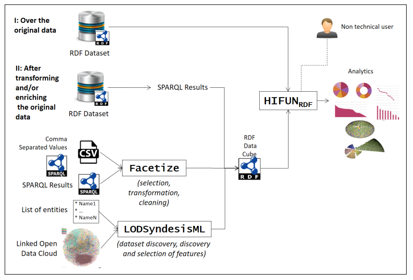
4. Using HIFUN as an Interface to RDF Dataset

There are several ways in which HIFUN can be used, such as for studying rewriting of analytic queries in the abstract [14] or for defining an approach to data exploration [39]. In this paper, we use HIFUN as a user-friendly interface for defining analytic queries over RDF data sets. To understand the proposed approach, consider a data source S with query language L (e.g., S could be a relational data set and L the SQL language). In order to use HIFUN as a user interface for S, we need to (a) define an analysis context, that is a subset D of S to be analyzed, and some attributes of D that are relevant for the analysis and (b) define a mapping of HIFUN queries to queries in L.

Defining a subset D of S can be done using a query of L and defining D to be its answer (i.e., D is defined as a view of S); and similarly, the attributes that are relevant to the analysis can be defined based on attributes of D already present in S. However, defining a mapping of HIFUN queries to queries in L might be a tedious task. In [39] such mappings have been defined from HIFUN queries to SQL queries and from HIFUN queries to MapReduce jobs.

The main objective of this paper is to define a user-friendly interface allowing users to perform analysis of RDF data sets. To this end, we use the HIFUN language as the interface. In other words, we consider the case where the data set S mentioned above is a set of RDF triples and its language L is the SPARQL language. Our main contributions are: (a) the proposal of tools for defining a HIFUN context from the RDF data set S and (b) defining a mapping from HIFUN queries to SPARQL queries. With these tools at hand, a user of the HIFUN interface can define an analysis context of interest over S and issue analytic queries using the HIFUN language. Each such query is then translated by the interface to a SPARQL query, which in turn is evaluated over the RDF triples of D and the answer is returned to the user.

5. Applicability of HIFUN over RDF

In Section 5.1 we discuss the prerequisites for applying HIFUN over RDF, and then (in Section 5.2) we describe two methods for applying HIFUN over RDF: over the original data (in Section 5.3), and after transforming the original data (in Section 5.4).

5.1. Prerequisites for Applying HIFUN over RDF Data

Two assumptions should hold to apply HIFUN over a data set D, (i) the unique identification of its data items and (ii) the functionality of its attributes.

RDF data. The first assumption, the unique identification of the data items, is satisfied by the RDF data, since each resource is identified by a distinct URI. Consequently, D can be any subset of the set of all the available URIs. The second assumption, the functionality of attributes, is partially satisfied by the RDF properties. The functional (i.e., owl:FunctionalProperty) or the effectively functional properties (i.e., even if they are not declared as functional, they are single-valued for the resources in the data set D) have only one unique value for each instance. However, there are also properties in RDF with (i) no or (ii) multiple values; a non-value property implies that a value may not exist (or it is unknown even if it exists) or it is incomplete, while a multi-valued infers that a property has more than one values for the same resource. Such cases require transforming the original data before applying HIFUN to it. These transformations can be made using the operators that will be described in Section 5.4.

RDF Schema. Each resource of an RDF schema is identified by a distinct URI; therefore, its data items are uniquely identified. However, a property (e.g., rdf:type, rdfs:subClassOf etc.) may appear more than once by relating different classes or classifying concepts in more than one classes (i.e., a class might be sub-class of several super-classes). Nevertheless, these relationships are considered distinct since they have different domain and/or range. Therefore, HIFUN allows analytics not only over the data, but over RDF schema(s) as well. Inference is supported, too, since it refers to automatic procedures that generate new relationships based on a set of rules; a process that is independent of HIFUN.

5.2. Methods to Apply HIFUN over RDF

We can identify two main methods for applying HIFUN over RDF:

I:

Defining an Analysis Context over the Original RDF Data. Here the user selects some properties, all satisfying the aforementioned assumptions. This is discussed in Section 5.3.

II:

Defining an Analysis Context after Transforming the Original RDF Data. Here the user transforms parts of the RDF graph in a way that satisfies the aforementioned assumptions. This is discussed in Section 5.4.

5.3. I: Defining an Analysis Context over the Original RDF Data

Definition 3

(Analysis Context). An analysis context C over RDF data is defined as a set of resources R to be analyzed along with a set of properties $p_1,p_2,...,p_n$ that are relevant for the analysis.

As the root of an analysis context in RDF can be selected any class (i.e., set of resources) of an RDF graph and as attributes any properties of that graph. For example, any of the classes “ex:Invoice”, “ex:Branch”, “ex:Product”, “ex:Brand”, “ex:Person”, “ex:Nationality” of Figure 2 can be selected as the root of the context, while any of the properties “ex:hasDate”, “ex:takesPlaceA”, “ex:delivers”, “ex:inQuantity”, “ex:Brand”, “ex:founder”, “ex:nationality” as the attributes of it.

5.4. II: Defining an Analysis Context after Transforming the Original RDF Data

A few feature operators that could be used for transforming the original (RDF) data to be in compliance with the assumptions of HIFUN are indicated in Table 1. That table lists the nine most frequent Linked Data-based Feature Creation Operators (for short FCOs), as defined in [40], and they have been re-grouped according to our requirements. $\mathcal{T}$ denotes a set of triples, P a set of properties and $p,p_1$, $p_2$ properties. In detail,

• $fc{o}_1$ suits to the normal case and it can be exploited to confirm that all the properties are functional e.g., the date that each product was delivered, the branch where each invoice took place. The value can be numerical or categorical.
• $fc{o}_2$ and $fc{o}_3$ relate to issues that concern missing and multi-valued properties and can be used for turning properties with empty values into integers.
• $fc{o}_4$ can be used for converting a multi-valued property to a set of single-valued features, e.g., one boolean feature for each nationality that a founder may have.
• $fc{o}_5$ and $fc{o}_6$ concern the degree of an entity and can be used to find the set of triples that contains a specific entity, defining its importance.
• $fc{o}_7$ to $fc{o}_9$ investigate paths in an RDF graph, e.g., whether at least one founder of a brand is “French”. It can be used for specifying a path (i.e., a sequence of properties $p_1,p_2,...,p_n$ etc.) and treat it as an individual property p.

Table 1. Feature Creation Operators.

id	Operator Defining ${\mathit{f}}_{\mathit{i}}$	Type	${\mathit{f}}_{\mathit{i}}\left(\mathit{e}\right)$
Plain selection of one property
1	p.value	num/categ	$f_i\left(e\right)=\left\{v\right|(e,p,v)\in \mathcal{T}\}$
For missing values and multi-valued properties
2	p.exists	boolean	$f_i\left(e\right)=1$ if $(e,p,o)$ or $(o,p,e)\in \mathcal{T}$, otherwise $f_i\left(e\right)=0$
3	p.count	int	$f_i\left(e\right)=\left|\left\{v\right|(e,p,v)\in \mathcal{T}\}\right|$
For multi-valued properties
4	p.values.AsFeatures	boolean	for each $v\in \left\{v\right|(e,p,v)\in \mathcal{T}\}$ we get the feature $f_{iv}\left(e\right)=1$ if $(e,p,v)$ or $(v,p,e)\in \mathcal{T}$, otherwise $f_{iv}\left(e\right)=0$
General ones
5	degree	double	$f_i\left(e\right)=\left|\{(s,p,o)\in \mathcal{T}|s=eoro=e\}\right|$
6	average degree	double	$f_i\left(e\right)=\frac{\left|triples\right(C\left)\right|}{\left|C\right|}$ s.t. $C=\left\{c\right|(e,p,c)\in \mathcal{T}\}$ and $triples\left(C\right)=\left\{\right(s,p,o)\in \mathcal{T}|s\in Coro\in C\}$
Indicative extensions for paths
7	p1.p2.exists	boolean	$f_i\left(e\right)=1$ if $\exists o2$ s.t. $\left\{\right(e,p1,o1),(o1,p2,o2\left)\right\}\subseteq \mathcal{T}$
8	p1.p2.count	int	$f_i\left(e\right)=\left|\left\{o2\right|(e,p1,o1),(o1,p2,o2)\in \mathcal{T}\}\right|$
9	p1.p2.value.maxFreq	num/categ	$f_i\left(e\right)=$ most frequent $o2$ in $\left\{o2\right|(e,p1,o1),(o1,p2,o2)\in \mathcal{T}\}$

Table 1. Feature Creation Operators.

id	Operator Defining ${\mathit{f}}_{\mathit{i}}$	Type	${\mathit{f}}_{\mathit{i}}\left(\mathit{e}\right)$
Plain selection of one property
1	p.value	num/categ	$f_i\left(e\right)=\left\{v\right|(e,p,v)\in \mathcal{T}\}$
For missing values and multi-valued properties
2	p.exists	boolean	$f_i\left(e\right)=1$ if $(e,p,o)$ or $(o,p,e)\in \mathcal{T}$, otherwise $f_i\left(e\right)=0$
3	p.count	int	$f_i\left(e\right)=\left|\left\{v\right|(e,p,v)\in \mathcal{T}\}\right|$
For multi-valued properties
4	p.values.AsFeatures	boolean	for each $v\in \left\{v\right|(e,p,v)\in \mathcal{T}\}$ we get the feature $f_{iv}\left(e\right)=1$ if $(e,p,v)$ or $(v,p,e)\in \mathcal{T}$, otherwise $f_{iv}\left(e\right)=0$
General ones
5	degree	double	$f_i\left(e\right)=\left|\{(s,p,o)\in \mathcal{T}|s=eoro=e\}\right|$
6	average degree	double	$f_i\left(e\right)=\frac{\left|triples\right(C\left)\right|}{\left|C\right|}$ s.t. $C=\left\{c\right|(e,p,c)\in \mathcal{T}\}$ and $triples\left(C\right)=\left\{\right(s,p,o)\in \mathcal{T}|s\in Coro\in C\}$
Indicative extensions for paths
7	p1.p2.exists	boolean	$f_i\left(e\right)=1$ if $\exists o2$ s.t. $\left\{\right(e,p1,o1),(o1,p2,o2\left)\right\}\subseteq \mathcal{T}$
8	p1.p2.count	int	$f_i\left(e\right)=\left|\left\{o2\right|(e,p1,o1),(o1,p2,o2)\in \mathcal{T}\}\right|$
9	p1.p2.value.maxFreq	num/categ	$f_i\left(e\right)=$ most frequent $o2$ in $\left\{o2\right|(e,p1,o1),(o1,p2,o2)\in \mathcal{T}\}$

These features can be used for deriving a new RDF dataset that will be analyzed with HIFUN. This transformation can be done by using SPARQL CONSTRUCT queries: Suppose that the pair $(R,F)$ expresses a context, where R is a set of resources and F the set of the features, the objects in R have. Then, the resources R, as well as the features F, can be defined by the triple patterns i.e., “?s ?p ?o” in the $CONSTRUCT$ clause of a SPARQL query, i.e., the bindings of “s” (or “o”) can correspond to the resources, whereas the bindings of “p” to the set of features. Alternatively, these features can be defined by queries, but instead of constructing the triples, the definition of the features can be included in the analytic queries in the form of nested queries (subqueries); in general any query translation method for virtual integration [41] can be used. A concrete example will be given in Section 6.6.

Finally, we should mention that the above list is by no means complete; the list of feature operators can be expanded to cover the requirements that arise.

6. Translation of HIFUN Queries to SPARQL

Here we focus on how to translate a HIFUN query, over an analysis context over RDF (case I), to a SPARQL query. Roughly, the grouping function will eventually yield variable(s) in the GROUP BY clause, the measuring function will yield at least one variable in the WHERE clause, and the aggregate operation corresponds to the appropriate aggregate SPARQL function in the SELECT clause (over the measuring variable). We explain the translation method gradually using examples, assuming the running example of Figure 2.

6.1. Simple Queries

Suppose that we would like to find the total quantities of products delivered to each branch. This query would be expressed in HIFUN as $(takesPlaceAt,inQuantity,SUM)$ and in SPARQL as (for reasons of brevity we assume the namespace prefix “ex” for each property of the following queries):

• SELECT ?x2 SUM(?x3)
  WHERE {
  ?x1 ex:takesPlaceAt ?x2 .
  ?x1 ex:inQuantity ?x3 .
  }
  GROUP BY ?x2

Therefore a HIFUN query (g, m, $op$) is translated to SPARQL as follows: the function g is translated to a triple pattern ?x1 g ?x2 (in the WHERE clause) and the variable ?x2 is added to the SELECT clause, and in the GROUP BY clause. The function m is translated to a triple pattern ?x1 m ?x ${}_N$ in the WHERE clause, where x ${}_N$ denotes a new variable. Finally, the function $op$ is translated to a $op\left(right\right(m\left)\right)$ in the SELECT clause, where $right\left(m\right)$ refers to the “right” variable of the triple pattern derived by the translation of m, i.e., to ?x${}_N$, in our example SUM(?x3).

6.2. Attribute-Restricted Queries

Suppose that we would like to find the total quantities of products, delivered to one particular branch, say branch1. This query would be expressed in HIFUN as

$(takesPlaceAt{/}_{branch1},inQuantity,SUM)$ and in SPARQL as:

• SELECT ?x2 SUM(?x3)
  WHERE {
  ?x1 ex:takesPlaceAt ?x2 .
  ?x1 ex:inQuantity ?x3 .
  ?x1 ex:takesPlaceAt branch1.
  }
  GROUP BY ?x2

Therefore for translating the HIFUN query ($g/v$, m, $op$) we translate the restriction v by adding in the WHERE clause the triple pattern ?x1 g v. Pleas note that here the restriction value refers to a URI. If that value had been represented with a literal, then a FILTER statement would have to be added in the WHERE clause. For example, consider the following example (where in this case the restriction is applied to the measuring function): Suppose that we would like to find the total quantities of products, delivered to each branch by considering only those invoices with quantity greater than or equal to 1. This query would be expressed in HIFUN as $(takesPlaceAt,inQuantity{/}_{>=1},SUM)$ and in SPARQL as:

• SELECT ?x2 SUM(?x3)
  WHERE {
  ?x1 ex:takesPlaceAt ?x2 .
  ?x1 ex:inQuantity ?x3 .
  FILTER(?x3 ≥ xsd:integer(“1”)).
  }
  GROUP BY ?x2

Consequently, a literal-attribute restriction in a HIFUN query (g, $m/cond$, $op$) would be translated by adding in the WHERE clause the following constraint FILTER($right\left(m\right)$$cond$).

6.3. Results-Restricted Queries

Suppose that we would like to find the total quantities of products, delivered to each branch, but only for branches with total quantity greater than 1000. This query would be expressed in HIFUN as, $(takesPlaceAt,inQuantity,SUM{/}_{>1000})$ and in SPARQL as:

• SELECT ?x2 SUM(?x3)
  WHERE {
  ?x1 ex:takesPlaceAt ?x2 .
  ?x1 ex:inQuantity ?x3 .
  }
  GROUP BY ?x2
  HAVING (SUM(?x3) > 1000)

Therefore for translating the HIFUN query (g, m, $op/cond$) we translate the restriction $cond$ by adding a HAVING clause with the following constraint HAVING $Right\left(m\right)$$cond$.

6.4. Complex Grouping Queries

A grouping (as well as a measuring) function in HIFUN can be more complex using the following operations on functions, as defined in [14]: composition (∘) and pairing (⊗). These operations form the so-called functional algebra [16] and they are well known, elementary operations.

6.4.1. Composition

Suppose that we ask for the total quantities of products delivered by brand. This query would be expressed in HIFUN as (brand ∘ delivers, inQuantity, SUM), and in SPARQL as:

• SELECT ?x3 SUM(?x4)
  WHERE {
  ?x1 ex:delivers ?x2 .
  ?x2 ex:brand ?x3 .
  ?x1 ex:inQuantity ?x4 .
  }
  GROUP BY ?x3

Therefore, a HIFUN query ($f_k$∘ ,..., ∘$f_2$∘$f_1$, m, op) would be translated as follows. At first note that if instead of the composition we had one function $f_1$, then it would be interpreted as a single query, i.e., we would add the triple pattern ?x1 $f_1$ ?x2 to the WHERE clause and the variable right($f_1$) would be added to the SELECT and to the GROUP BY clause. If we had the composition of two functions ($f_2$∘$f_1$), then we would add the triple patterns ?x1 $f_1$ right($f_1$) and right($f_1$) $f_2$ ?xf2r (where xf2r is a brand new variable) to the WHERE clause and the variable right($f_2$) to the SELECT and to the GROUP BY clause.

Now suppose that the composition function comprises k functions, ($f_k$∘, ..., ∘$f_2$∘$f_1$), which would be translated to the triple patterns ?x1 $f_1$ right($f_1$), right($f_1$) $f_2$ right($f_2$), ..., right($f_{k-1}$) $f_k$ right($f_k$) to the WHERE clause and the variable right($f_k$) to the SELECT and to the GROUP BY clause. If we added one more function to the composition (reaching to k+1 functions), i.e., ($f_{k+1}$∘$f_k$∘, ..., ∘$f_2$∘$f_1$), we would have to add the triple pattern right($f_k$) $f_{k+1}$$?xnew$ (where $?xnew$ is a brand new variable) to the WHERE clause and to replace the variable right($f_k$) with the right($f_{k+1}$) in the SELECT and in the GROUP BY clause.

Now we shall provide an example of composition with a derived attribute. Suppose that we ask for the total quantities of products delivered by month. This query would be expressed in HIFUN as (month ∘ date, inQuantity, SUM) and in SPARQL as:

• SELECT month(?x2) SUM(?x3)
  WHERE {
  ?x1 ex:hasDate ?x2 .
  ?x1 ex:inQuantity ?x3 .
  }
  GROUP BY month(?x2)

Therefore, a HIFUN query $(f\circ g,m,op)$, where the attribute f derives from g, would be translated by adding to the WHERE clause the triple pattern ?x1 g ?xf2r (where ?xf2r is a brand new variable). Then, f would be derived from $right\left(g\right)$ by adding to the SELECT and to the GROUP BY clauses a SPARQL build-in function i.e., f(right(g)) (in our example month(?x2)); this function would extract the value f from that of $right\left(g\right)$.

6.4.2. Pairing

Suppose that we would like to find the total quantities delivered by branch and product. This query would be expressed in HIFUN as $\left(\right(takesPlaceAt\otimes delivers),inQuantity,SUM)$ and in SPARQL as:

• SELECT ?x2 ?x4 SUM(?x3)
  WHERE {
  ?x1 ex:takesPlaceAt ?x2 .
  ?x1 ex:inQuantity ?x3 .
  ?x1 ex:delivers ?x4.
  }
  GROUP BY ?x2 ?x4

Therefore, a HIFUN query ($f_k$⊗ ,..., ⊗$f_2$⊗$f_1$, m, op) would be translated as follows: we would add (i) the triple patterns ?x1 $f_1$ right($f_1$), ?x1 $f_2$ right($f_2$), ..., ?x1 $f_k$ right($f_k$) to the WHERE clause and (iii) the variables right($f_1$), right($f_2$), ..., right($f_k$) to the SELECT and to the GROUP BY clauses. In other words, we would join the pairing functions i.e., $f_1$, $f_2$,..., $f_k$ on their shared variable i.e., $?x1$.

6.5. The Full Algorithm for Translating a HIFUN Query to a SPARQL Query

Let us now describe the full translation algorithm. Let $q=(gE/rg,mE/rm,opE/ro)$ be a HIFUN query where

• $gE$ is the grouping expression,
• $mE$ is the measuring expression,
• $opE$ is the operation expression, and
• $rg$ is a restriction on the grouping expression,
• $rm$ is a restriction on he measuring expression, and
• $ro$ is a restriction on the operation expression.

The final query is constructed by concatenating strings as shown below:

Q = “SELECT” +retVars(gE) + “ ”+opE(mE) +“\n”

+ “WHERE {” +“ \n”

+ triplePatterns(gE) +“ \n”

+ triplePatterns(mE) +“ \n”

+ “}” +“ \n”

+ “GROUP BY " +retVars(gE) +“ \n"

+“ HAVING " +restr($Q_{ans}$)

The way the variables $retVars\left(gE\right)$, $opE\left(mE\right)$, $triplePatterns\left(gE\right)$, $triplePatterns\left(mE\right)$, $retVars\left(gE\right)$, and $restr\left(Q_{ans}\right)$ are constructed, is described next

1.

We start the translation with the grouping expression $gE$ by creating the string format of the triple patterns in which the terms $g_i$ of $gE$ participates, triplePatterns(gE) += $?x_i$$g_i$$right\left(g_i\right)$, as described in Section 6.1 and Section 6.4.

If $gE$ contains any restriction $rg$ we supplementarily create the string format of the triple pattern expressing that constraint:

1.1.

if $rg$ refers to a URI, then triplePatterns(gE) += $?x_i$$g_i$$rg$,

1.2.

if $rg$ is represented with a LITERAL, then triplePatterns(gE) += FILTER($right\left(g_i\right)$$rg$), as described in Section 6.2.

2.

We proceed with the translation of the measuring expression $mE$ by creating the string format of the triple patterns in which the terms $m_i$ of $mE$ participates, triplePatterns(mE) += $x_i$$m_i$$right\left(m_i\right)$. Since this expression can also be complex, the translation is made as described in Section 6.1 and Section 6.4.

If $mE$ contains any restriction $rm$ we supplementarily create the string format of the triple pattern expressing that constraint:

2.1.

if $rm$ refers to a URI, then triplePatterns(mE) += $?x_i$$m_i$$rm$,

2.2.

if $rm$ is represented with a LITERAL, then triplePatterns(mE) += FILTER($right\left(m_i\right)$$rm$), as described in Section 6.2.

3.

Following, we create the string format of the returned variables, retVars(gE) += $right\left(g_i\right)$ as described in Section 6.1 and Section 6.4.

4.

At last, we translate the aggregate expression $opE$ by creating the string format of the operation $op$ applied over the values of $mE$, i.e., $opE\left(mE\right)$ = op($right\left(m_i\right)$), as described in  Section 6.1.

5.

Optionally, if any restrictions $re$ are applied to the final answers $Q_{ans}$, then we create the string format of the condition expressing these constraints, restr($Q_{ans}$) = right($m_i$) re as described in Section 6.3.

To give an example suppose that we would like to find he total quantities by branch and brand only for the month of January, by considering only (a) the invoices with quantity greater than or equal to 2, and (b) the branches with total quantity greater than 1000. This query would be expressed in HIFUN as

$(takesPlaceAt\otimes (brand\circ delivers)){/}_{month=01},inQuantit{y}_{>=2},SUM{/}_{>1000})$ and (by following the above translation process) in SPARQL as:

• SELECT ?x2 ?x5 SUM(?x3)
  WHERE {
  ?x1 ex:takesPlaceAt ?x2 .
  ?x1 ex:inQuantity ?x3 .
  ?x1 ex:delivers ?x4 .
  ?x4 ex:brand ?x5 .
  ?x1 ex:hasDate ?x6 .
  FILTER((MONTH(?x6) = 01) && (?x3 $>=$ xsd:integer("2")))
  }
  GROUP BY ?x2 ?x5
  HAVING (SUM(?x3) > 1000)

The pseudocode of the algorithm that defines the variables $retVars\left(gE\right)$, $opE\left(mE\right)$, $triplePatterns\left(gE\right)$, $triplePatterns\left(mE\right)$, $retVars\left(gE\right)$, and $restr\left(Q_{ans}\right)$, for the simple case, where the HIFUN query does not contain compositions and pairings, is given in Algorithm 1.

Algorithm 1 Algorithm for computing the components of the translated query for the Simple Case

However, in the general case we may have compositions in grouping, measuring and restrictions. They way compositions are translated is described in Algorithm 2. The extension of the composition algorithm that supports also derived attributes is given in Algorithm 3. Please note that all predefined functions of SPARQL with one parameter can be used straightforwardly as derived attributes.

In addition, Algorithm 2 shows how pairing is translated. If $gE$ involves both pairing and composition it will have the form $g{c}_1\otimes \dots \otimes g{c}_k$ where each $g{c}_i$ can be an individual function or a composition of functions. Such expressions are translated as follows: translate($gE$) = translatePairing(translateComposition($g{c}_1$) $\otimes \dots \otimes$ translateComposition($g{c}_k$)). The exact steps for translating pairing of compositions are given in Algorithm 2-PairingAndComposition.

Algorithm 4 is the algorithm for the general case, where compositions can occur in the restrictions too. Notice that now $rg$ is not necessarily a single URI or literal, but a path expression that ends with a URI or literal. In this scenario, instead of $(takesPlaceAt{/}_{‘‘branch1"},inQuantity,SUM)$ we write $(takesPlaceAt{/}_{takesPlaceAt=branch1},inQuantity,SUM)$, and we now support expressions of the form $(takesPlaceAt{/}_{location\circ takesPlaceAt=ex:Athens},inQuantity,SUM)$. The path of the restriction is not necessarily the same with that of the grouping, e.g., we can get the sum of quantities grouped by brand, only for those branches that are located in Athens by the following query $(brand\circ delivers{/}_{location\circ takesPlaceAt=Athens},inQuantity,sum)$. Such expressions are supported also for the restriction $rm$ of the measuring function.

Algorithm 2 Auxiliary algorithms for compositions and pairings

Algorithm 3 Algorithm for composition if derived attributes are involved

Algorithm 4 Algorithm for computing the components of the translated query for the General case

The above translation process can also support cases where the set of resources R of an analysis context is defined by one unary query, a query that returns a set of URIs. If $q_{str}\left(R\right)$ denotes the string of that query, then $q_{str}\left(R\right)$ can be used as the starting point of the above (query translation) process, i.e., the triple patterns of $q_{str}\left(R\right)$ will be the first to be added to the triples patterns of our query Q; the only constraint is that $q_{str}\left(R\right)$ should have one variable ?x1 in the select clause.

In general, the translation algorithm works for all possible HIFUN queries.

6.6. Cases Where the Prerequisites of HIFUN Are Not Satisfied

Let us now discuss the problem of translation for the case where the requirements for applying HIFUN (as described in Section 5.1) do not hold, as well as when features (as described in Section 5.4) are required.

Consider that the running example of Figure 2 contained a property “ex:birthYear” with domain the class “ex:Person” and range an integer-typed literal. Now suppose that we would like to compute a single number being the average birth year of the founders of the products that were sold. Here the problem of incomplete information arises, i.e., the dataset may not contain information about the founders of all products, let alone their birth year, therefore the path $delivers.brand.founder.birthYear$ will not be “applicable” to several invoices. If we formulate such a query in HIFUN, it will be translated to a SPARQL query that will be evaluated successfully; however the results will not be complete, i.e., only the invoices for which the path $delivers.brand.founder.birthYear$ exists will be considered.

Moreover, we may encounter the problem of multiple values, i.e., when a brand was founded by more than one person. In that case, even if our dataset contained complete information, the path $delivers.brand.founder.birthYear$ would not be functional. If we formulate such a query in HIFUN, it will be translated to a SPARQL query that will be evaluated successfully; however the results will not be accurate, i.e., all paths will be taken into account; valuating more than one birth year per product, not only one birth year per product.

If we wanted to associate each product with only one birth year (before taking the average over all products), then in case of multiple founders, we could define a feature that computes the average birth year of each individual product. Having this feature enables the subsequent formulation of a HIFUN query, that would compute the accurate answer. There are several possible methods to define such features using the query language (as mentioned in Section 5.4). In our example, the average birth year of the founder(s) for each individual product can be computed by one query that yields a variable for that feature:

• $qf$ =
  SELECT ?x2 AVG(?x5) as productFoundBirthYearAvg
  WHERE {
  ?x1 ex:delivers ?x2 .
  ?x2 ex:brand ?x3 .
  ?x3 ex:founder ?x4 .
  ?x4 ex:birthYear ?x5 .
  }
  GROUP BY ?x2

To compute accurately that we want to (i.e., average birth year of the founders of the products that were sold), we can exploit the notion of SPARQL subqueries (that was mentioned in the last part of Section 5.4) to “embded” the aforementioned query $qf$.

Please note that subqueries are a way to embed SPARQL queries inside other queries to allow the expression of requests that are not possible otherwise. Subqueries are evaluated first and then the outer query is applied to their results Only variables projected out of the subquery (i.e., appearing in its SELECT clause) are visible to the outer query. Therefore the features can be expressed as subqueries that can be placed in the WHERE clause.

In our case, the HIFUN query that computes the average birth year of the founders of the products would have the following form: $Q=(ϵ,product.productFoundBirthYearAvg,AVG)$, where $productFoundBirthYearAvg$ is a feature (according to Table 1 we would write $productFoundBirthYearAvg=delivers.brand.founder.birthYear.avg$); note that $ϵ$ denotes the empty grouping function, since in our example we do not want to group the results, just to apply $AVG$ to the entire set. To compute this feature we can use a subquery that returns two variables, one for the objects and one for the corresponding feature value, say $vf1$ and $vf2$ respectively, while ensuring that $vf1$ should the same with the variable used in the outer query for these objects. In our example, the corresponding SPARQL query that computes the sought answer (where the subquery provides two variables), is the following:

• SELECT AVG(?productFoundBirthYearAvg)
  WHERE {
       ?x1 ex:delivers ?x2 .
       {
         SELECT ?x2 (AVG(?x5) AS ?productFoundBirthYearAvg)
         WHERE {
           ?x1 ex:delivers ?x2 .
           ?x2 ex:brand ?x3 .
           ?x3 ex:founder ?x4 .
           ?x4 ex:birthYear ?x5 .
         }
         GROUP BY ?x2
       }
  }

This example showcased how we can compute accurate results if the paths that are involved in the HIFUN query are not functional.

6.7. Analytics and RDF Schema Semantics

The translation of SPARQL allows leveraging the RDF Schema semantics, specifically the RDF Schema-related inference that is supported by SPARQL. To give a simple indicative example, consider two properties directorOf and worksAt such that (directorOf,rdfs:subPropertyOf,worksAt) and suppose the following data:

• (p1,directorOf,brand1)
  (p2,worksAt,brand1)
  (p3,worksAt,brand1)
  (p4,worksAt,brand1)
  (p1,livesAt,Athens)
  (p2,livesAt,Rhodes)
  (p3,livesAt,Corfu),
  (p4,livesAt,Corfu)

If we want to compute the locations where the persons related to brand1 work at, and how many live at each place, we could use the following HIFUN query $(workAt,livesAt,COUNT)$. If the inference of SPARQL is enabled, then the translated query will return

• Athens,1
  Rhodes,1
  Corfu,2

The key point is that the location of the director will be considered, since it is inferred that (p1,worksAt,brand1). Such inference would not be possible if we translated the data to the relational model.

The ability to leverage the inference rules of RDF Schema in the context of analytic queries is especially important for datasets which are described with ontologies that contain high number of subClassOf and subPropertyOf relationships for achieving semantic interoperability across various datasets, like those in the cultural and historic domain [7,42].

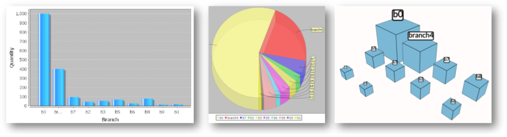
7. On Interactivity

As described in the introductory section, and illustrated in Figure 1, our ultimate objective is to provide a user friendly method for interactive analytics over any RDF graph. This requires:

${\mathcal{S}}_{①ctx}$

 An interactive method for specifying an Analysis Context. Recall that (according to Definition 3), an analysis context C over RDF data is defined as a set of resources R to be analyzed along with a set of properties $p_1,p_2,...,p_n$ that are relevant for the analysis.

${\mathcal{S}}_{②q}$

  An interactive method for formulating the desired HIFUN query $q=(g,m,op)$, i.e., a method to select g, m, and $op$.

${\mathcal{S}}_{③tr}$

  A method to translate the HIFUN query to SPARQL.

${\mathcal{S}}_{④vis}$

 A method for visualizing the results of the SPARQL query that is derived by translating q.

As regards ${\mathcal{S}}_{①ctx}$, the analysis context can be specified over the original data (Section 5.3), or after a transformation (Section 5.4). In the former case, the user does not have to do anything: all resources of the RDF dataset and all properties can be exploited as an analysis context. In the latter case the intended transformation can be made by tools like LODSyndesisML [40] that allows the user to interactively select the desired features. The output of this step can be either (a) a csv file or an RDF file in RDF Data Cube format that contains the materialization of the defined features, or (b) a set of feature specifications each being a pair (feature name, SPARQL query) which will be exploited in the translation process as discussed in the last part of Section 5.4 and in Section 6.6.

As regards ${\mathcal{S}}_{②q}$, and assuming that an analysis context has been specified, we developed a tool, called HIFUN ${}_{RDF}$, where user is asked to select the functions of a HIFUN query i.e., (i) the grouping function, (ii) the measuring function, (iii) the aggregate operation, and optionally, (iv) set restrictions to the grouping, the measuring functions or to the final results. The above are accomplished by interactively selecting the desired properties, i.e., the user does not have to know the SPARQL syntax. Currently, this tool loads data represented in the RDF Data Cube format and stores them in a triplestore, however this period we are extending this tool for supporting any RDF file (not only files in RDF Data Cube format).

As regards ${\mathcal{S}}_{③tr}$, we implemented the translation method described in Section 6. Please note that the cost of the translation of a HIFUN query to SPARQL is negligible (the translation has linear complexity with respect to the size of the HIFUN string; it does not depend on the size of the data).

The translated to SPARQL query is then executed on the triple store OpenLink Virtuoso (https://virtuoso.openlinksw.com/) (where the input data has been uploaded) and the returned results are displayed and saved in a “.csv” file in the form of - $va{r}_1,va{r}_2,...,va{r}_i$, TOTALS.

As regards ${\mathcal{S}}_{④vis}$, we embedded in HIFUN ${}_{RDF}$ the jfreechart library (https://www.jfree.org/jfreechart) for reading the results of the SPARQL query and preparing various charts including line, bar, pie and 3D pie charts. Three screenshots are shown in Figure 4 that visualize the results of the query “total quantities by branch” over a synthetic RDF dataset that uses the same schema with our running example.

The indicative flows that are possible with this implementation, are illustrated in Figure 5. The figure includes a workflow where the process starts with selecting the data set the user wants to analyze using tools like Facetize [43] and LODSyndesisML [40], suitable for discovering, cleaning, organizing data in hierarchies. etc. Then, this data is converted into the RDF Data Cube format and is loaded in HIFUN ${}_{RDF}$. HIFUN ${}_{RDF}$ is not yet public, a public version will be released after tackling the extensions described next in Section 7.1.

7.1. Future Work

Currently we are working on a second implementation that will support, in a single system, and interactively, all steps of the process for ${\mathcal{S}}_{①ctx}$ to ${\mathcal{S}}_{④vis}$. The objective is to provide a unified interface that will enable the user to (i) select the RDF file or triple store (s)he wants to analyze, (ii) specify and change the analysis context on the fly (and provide the capability to define features as described in Section 5.4), and (iii) formulate an analytical query by defining its components by selecting the applicable properties. Then, the system will translate the query and finally visualize the results in tabular form as well as in various other forms (like those described in [44]) including 3D (by extending the work of [45] (http://www.ics.forth.gr/isl/3DLod/)) allowing the user to explore them, intuitively. For steps (ii) and (iii) we plan to investigate extending the core model for exploratory search over RDF that is described in [12] (for exploiting its capabilities of forming conditions that involve paths and complex expressions), with actions for supporting ${\mathcal{S}}_{①ctx}$ and ${\mathcal{S}}_{②q}$(that are not supported by that model). That will enable the user to specify interactively and with simple clicks complex restrictions that may concern the set of resources of the analysis context, and/or the various restrictions of the analytic query (of grouping or measuring functions, or of the final results).

Finally, we should mention that an interactive system for analytics that uses HIFUN as the intermediate layer, enables the formulation of analytic queries over data sources with different data models and query languages, since there are already mappings of HIFUN to SQL (for relational sources), and to MapReduce using SPARK [46], thus our work enables applying that model over RDF data sources too.

8. Concluding Remarks

In this paper, we elaborated on the general problem of providing interactive analytics over RDF data. We showed the motivation for this direction, we described the main requirements and challenges, and we discussed the work that has been done in this area. Subsequently we investigated whether HIFUN, a functional query language for analytics, can be used as a means for formulating analytic queries over RDF data in a flexible manner. To this end, we analyzed the applicability of HIFUN over RDF, we described various methods that can be used to apply HIFUN over such data, and then we focused on the problem of translating HIFUN queries to SPARQL queries, starting from simple queries and ending up to complex queries. We discussed what happens when HIFUN cannot be applied, and how features can be employed to tackle properties and paths that are not functional. The presented query translation approach does not require transforming or moving the data, and can leverage the inference that is provided by SPARQL. Subsequently we described how this approach can be exploited in an interactive context and we described our first implementation. Overall, we have shown that it is possible to provide a method for formulating complex analytic queries over RDF that is based on a few and basic concepts, those of HIFUN. In the future, we plan to implement a fully interactive system that will support all steps of the query formulation and visualization process and elaborate further on the interactivity of the approach.

References

- Mountantonakis, M.; Tzitzikas, Y. Large-scale Semantic Integration of Linked Data: A Survey. ACM Comput. Surv. (CSUR) 2019, 52, 103. [Google Scholar] [CrossRef]
- Bizer, C.; Lehmann, J.; Kobilarov, G.; Auer, S.; Becker, C.; Cyganiak, R.; Hellmann, S. DBpedia-A crystallization point for the Web of Data. J. Web Semant. 2009, 7, 154–165. [Google Scholar] [CrossRef]
- Vrandečić, D.; Krötzsch, M. Wikidata: A free collaborative knowledgebase. Commun. ACM 2014, 57, 78–85. [Google Scholar] [CrossRef]
- Wishart, D.S.; Feunang, Y.D.; Guo, A.C.; Lo, E.J.; Marcu, A.; Grant, J.R.; Sajed, T.; Johnson, D.; Li, C.; Sayeeda, Z.; et al. DrugBank 5.0: A major update to the DrugBank database for 2018. Nucleic Acids Res. 2018, 46, D1074–D1082. [Google Scholar] [CrossRef] [PubMed]
- Tzitzikas, Y.; Marketakis, Y.; Minadakis, N.; Mountantonakis, M.; Candela, L.; Mangiacrapa, F.; Pagano, P.; Perciante, C.; Castelli, D.; Taconet, M.; et al. Methods and Tools for Supporting the Integration of Stocks and Fisheries. In Chapter in Information and Communication Technologies in Modern Agricultural Development; Springer: Berlin/Heidelberg, Germany, 2019. [Google Scholar]
- Jaradeh, M.Y.; Oelen, A.; Farfar, K.E.; Prinz, M.; D’Souza, J.; Kismihók, G.; Stocker, M.; Auer, S. Open Research Knowledge Graph: Next Generation Infrastructure for Semantic Scholarly Knowledge. In Proceedings of the 10th International Conference on Knowledge Capture, Marina Del Rey, CA, USA, 19–21 November 2019; pp. 243–246. [Google Scholar]
- Koho, M.; Ikkala, E.; Leskinen, P.; Tamper, M.; Tuominen, J.; Hyvönen, E. WarSampo Knowledge Graph: Finland in the Second World War as Linked Open Data. Semant. Web Interoper. Usability Appl. 2020. [Google Scholar] [CrossRef]
- Dimitrov, D.; Baran, E.; Fafalios, P.; Yu, R.; Zhu, X.; Zloch, M.; Dietze, S. TweetsCOV19—A Knowledge Base of Semantically Annotated Tweets about the COVID-19 Pandemic. In Proceedings of the 29th ACM International Conference on Information and Knowledge Management (CIKM 2020), Virtual Event, Galway, Ireland, 19–23 October 2020. [Google Scholar]
- COVID-19 Open Research Dataset (CORD-19). 2020. Available online: https://www.semanticscholar.org/cord19 (accessed on 23 January 2021).
- Raphaël, G.; Franck, M.; Fabien, G. CORD-19 Named Entities Knowledge Graph (CORD19-NEKG). 2020. Available online: https://zenodo.org/record/3827449#.YA5dhBYRXIU (accessed on 23 January 2021).
- Nikas, C.; Kadilierakis, G.; Fafalios, P.; Tzitzikas, Y. Keyword Search over RDF: Is a Single Perspective Enough? Big Data Cogn. Comput. 2020, 4, 22. [Google Scholar] [CrossRef]
- Tzitzikas, Y.; Manolis, N.; Papadakos, P. Faceted exploration of RDF/S datasets: A survey. J. Intell. Inf. Syst. 2017, 48, 329–364. [Google Scholar] [CrossRef]
- Kritsotakis, V.; Roussakis, Y.; Patkos, T.; Theodoridou, M. Assistive Query Building for Semantic Data. In Proceedings of the SEMANTICS Posters&Demos, Vienna, Austria, 10–13 September 2018. [Google Scholar]
- Spyratos, N.; Sugibuchi, T. HIFUN-a high level functional query language for big data analytics. J. Intell. Inf. Syst. 2018, 51, 529–555. [Google Scholar] [CrossRef]
- Papadaki, M.E.; Tzitzikas, Y.; Spyratos, N. Analytics over RDF Graphs. In Proceedings of the International Workshop on Information Search, Integration, and Personalization, Heraklion, Greece, 9–10 May 2019. [Google Scholar]
- Spyratos, N. A functional model for data analysis. In Proceedings of the International Conference on Flexible Query Answering Systems, Milan, Italy, 7–10 June 2006. [Google Scholar]
- Tzitzikas, Y.; Allocca, C.; Bekiari, C.; Marketakis, Y.; Fafalios, P.; Doerr, M.; Minadakis, N.; Patkos, T.; Candela, L. Integrating heterogeneous and distributed information about marine species through a top level ontology. In Proceedings of the Research Conference on Metadata and Semantic Research, Thessaloniki, Greece, 19–22 November 2013. [Google Scholar]
- Isaac, A.; Haslhofer, B. Europeana linked open data—Data. europeana. eu. Semant. Web 2013, 4, 291–297. [Google Scholar] [CrossRef]
- Mountantonakis, M.; Tzitzikas, Y. On measuring the lattice of commonalities among several linked datasets. Proc. VLDB Endow. 2016, 9, 1101–1112. [Google Scholar] [CrossRef]
- Mountantonakis, M.; Tzitzikas, Y. Scalable Methods for Measuring the Connectivity and Quality of Large Numbers of Linked Datasets. J. Data Inf. Qual. (JDIQ) 2018, 9, 1–49. [Google Scholar] [CrossRef]
- Roatis, A. Analysing RDF Data: A Realm of New Possibilities. ERCIM News. 2014. Available online: https://ercim-news.ercim.eu/en96/special/analysing-rdf-data-a-realm-of-new-possibilities (accessed on 23 January 2021).
- Kämpgen, B.; O’Riain, S.; Harth, A. Interacting with statistical linked data via OLAP operations. In Proceedings of the Extended Semantic Web Conference, Crete, Greece, 27–31 May 2012. [Google Scholar]
- Etcheverry, L.; Vaisman, A.A. QB4OLAP: A new vocabulary for OLAP cubes on the semantic web. In Proceedings of the Third International Conference on Consuming Linked Data, Boston, MA, USA, 12 November 2012. [Google Scholar]
- Azirani, E.A.; Goasdoué, F.; Manolescu, I.; Roatiş, A. Efficient OLAP operations for RDF analytics. In Proceedings of the 2015 31st IEEE International Conference on Data Engineering Workshops, Seoul, Korea, 13–17 April 2015; pp. 71–76. [Google Scholar]
- Ruback, L.; Pesce, M.; Manso, S.; Ortiga, S.; Salas, P.E.R.; Casanova, M.A. A mediator for statistical linked data. In Proceedings of the 28th Annual ACM Symposium on Applied Computing, Coimbra, Portugal, 18–22 March 2013. [Google Scholar]
- Etcheverry, L.; Vaisman, A.A. Enhancing OLAP analysis with web cubes. In Proceedings of the Extended Semantic Web Conference, Crete, Greece, 27–31 May 2012. [Google Scholar]
- Zhao, P.; Li, X.; Xin, D.; Han, J. Graph cube: On warehousing and OLAP multidimensional networks. In Proceedings of the 2011 ACM SIGMOD International Conference on Management of Data, Athens, Greece, 12–16 June 2011. [Google Scholar]
- Benatallah, B.; Motahari-Nezhad, H.R. Scalable graph-based OLAP analytics over process execution data. Distrib. Parallel Databases 2016, 34, 379–423. [Google Scholar]
- Wang, K.; Xu, G.; Su, Z.; Liu, Y.D. GraphQ: Graph Query Processing with Abstraction Refinement—Scalable and Programmable Analytics over Very Large Graphs on a Single {PC}. In Proceedings of the 2015 Annual Technical Conference 15, Santa Clara, CA, USA, 8–10 July 2015. [Google Scholar]
- Zapilko, B.; Mathiak, B. Performing statistical methods on linked data. In Proceedings of the International Conference on Dublin Core and Metadata Applications, The Hague, The Netherlands, 21–23 September 2011. [Google Scholar]
- Olston, C.; Reed, B.; Srivastava, U.; Kumar, R.; Tomkins, A. Pig latin: A not-so-foreign language for data processing. In Proceedings of the 2008 ACM SIGMOD International Conference on Management of Data, Vancouver, BC, Canada, 9–12 June 2008. [Google Scholar]
- Thusoo, A.; Sarma, J.S.; Jain, N.; Shao, Z.; Chakka, P.; Zhang, N.; Antony, S.; Liu, H.; Murthy, R. Hive-a petabyte scale data warehouse using hadoop. In Proceedings of the 2010 IEEE 26th International Conference on Data Engineering (ICDE 2010), Long Beach, CA, USA, 1–6 March 2010. [Google Scholar]
- Etcheverry, L.; Vaisman, A.A. Querying Semantic Web Data Cubes. In Proceedings of the Alberto Mendelzon International Workshop on Foundations of Data Management, Panama City, Panama, 8–10 May 2016. [Google Scholar]
- Etcheverry, L.; Vaisman, A.A. Efficient Analytical Queries on Semantic Web Data Cubes. J. Data Semant. 2017, 6, 199–219. [Google Scholar] [CrossRef] [Green Version]
- Colazzo, D.; Goasdoué, F.; Manolescu, I.; Roatiş, A. RDF analytics: Lenses over semantic graphs. In Proceedings of the 23rd International Conference on World Wide Web, Seoul, Korea, 7–11 April 2014. [Google Scholar]
- Diao, Y.; Guzewicz, P.; Manolescu, I.; Mazuran, M. Spade: A modular framework for analytical exploration of RDF graphs. In Proceedings of the VLDB Endowment 2019, Los Angeles, CA, USA, 26–30 August 2019. [Google Scholar]
- Antoniou, G.; Van Harmelen, F. A Semantic Web Primer; MIT Press: Cambridge, MA, USA, 2004. [Google Scholar]
- Mountantonakis, M.; Tzitzikas, Y. LODsyndesis: Global Scale Knowledge Services. Heritage 2018, 1, 335–348. [Google Scholar] [CrossRef] [Green Version]
- Spyratos, N.; Sugibuchi, T. Data Exploration in the HIFUN Language. In Proceedings of the International Conference on Flexible Query Answering Systems, Amantea, Italy, 2–5 July 2019. [Google Scholar]
- Mountantonakis, M.; Tzitzikas, Y. How linked data can aid machine learning-based tasks. In Proceedings of the International Conference on Theory and Practice of Digital Libraries, Thessaloniki, Greece, 18–21 September 2017. [Google Scholar]
- Mami, M.N.; Graux, D.; Thakkar, H.; Scerri, S.; Auer, S.; Lehmann, J. The query translation landscape: A survey. arXiv 2019, arXiv:1910.03118. [Google Scholar]
- Fafalios, P.; Petrakis, C.; Samaritakis, G.; Doerr, K.; Tzitzikas, Y.; Doerr, M. FastCat: Collaborative Data Entry and Curation for Semantic Interoperability in Digital Humanities. ACM J. Comput. Cult. Herit. 2021. accepted for publication. [Google Scholar]
- Kokolaki, A.; Tzitzikas, Y. Facetize: An Interactive Tool for Cleaning and Transforming Datasets for Facilitating Exploratory Search. arXiv 2018, arXiv:1812.10734. [Google Scholar]
- Andrienko, G.; Andrienko, N.; Drucker, S.; Fekete, J.D.; Fisher, D.; Idreos, S.; Kraska, T.; Li, G.; Ma, K.L.; Mackinlay, J.; et al. Big Data Visualization and Analytics: Future Research Challenges and Emerging Applications. In Proceedings of the BigVis 2020: Big Data Visual Exploration and Analytics, Copenhagen, Denmark, 30 March 2020. [Google Scholar]
- Papadaki, M.E.; Papadakos, P.; Mountantonakis, M.; Tzitzikas, Y. An Interactive 3D Visualization for the LOD Cloud. In Proceedings of the EDBT/ICDT Workshops, Vienna, Austria, 26 March 2018. [Google Scholar]
- Zervoudakis, P.; Kondylakis, H.; Plexousakis, D.; Spyratos, N. Incremental Evaluation of Continuous Analytic Queries in HIFUN. In Proceedings of the International Workshop on Information Search, Integration, and Personalization, Heraklion, Greece, 9–10 May 2019; pp. 53–67. [Google Scholar]
Publisher’s Note: MDPI stays neutral with regard to jurisdictional claims in published maps and institutional affiliations. |
© 2021 by the authors. Licensee MDPI, Basel, Switzerland. This article is an open access article distributed under the terms and conditions of the Creative Commons Attribution (CC BY) license (http://creativecommons.org/licenses/by/4.0/).
Share and Cite
Papadaki, M.-E.; Spyratos, N.; Tzitzikas, Y. Towards Interactive Analytics over RDF Graphs. Algorithms 2021, 14, 34. https://doi.org/10.3390/a14020034
Papadaki M-E, Spyratos N, Tzitzikas Y. Towards Interactive Analytics over RDF Graphs. Algorithms. 2021; 14(2):34. https://doi.org/10.3390/a14020034
Chicago/Turabian StylePapadaki, Maria-Evangelia, Nicolas Spyratos, and Yannis Tzitzikas. 2021. "Towards Interactive Analytics over RDF Graphs" Algorithms 14, no. 2: 34. https://doi.org/10.3390/a14020034
APA StylePapadaki, M.-E., Spyratos, N., & Tzitzikas, Y. (2021). Towards Interactive Analytics over RDF Graphs. Algorithms, 14(2), 34. https://doi.org/10.3390/a14020034