Article

Disjoint Tree Mergers for Large-Scale Maximum Likelihood Tree Estimation

Department of Computer Science, University of Illinois Urbana-Champaign, Urbana, IL 61801, USA
*
Author to whom correspondence should be addressed.
Algorithms 2021, 14(5), 148; https://doi.org/10.3390/a14050148
Submission received: 31 March 2021 / Revised: 26 April 2021 / Accepted: 4 May 2021 / Published: 7 May 2021
(This article belongs to the Special Issue Algorithms in Computational Biology)

Abstract

:
The estimation of phylogenetic trees for individual genes or multi-locus datasets is a basic part of considerable biological research. In order to enable large trees to be computed, Disjoint Tree Mergers (DTMs) have been developed; these methods operate by dividing the input sequence dataset into disjoint sets, constructing trees on each subset, and then combining the subset trees (using auxiliary information) into a tree on the full dataset. DTMs have been used to advantage for multi-locus species tree estimation, enabling highly accurate species trees at reduced computational effort, compared to leading species tree estimation methods. Here, we evaluate the feasibility of using DTMs to improve the scalability of maximum likelihood (ML) gene tree estimation to large numbers of input sequences. Our study shows distinct differences between the three selected ML codes—RAxML-NG, IQ-TREE 2, and FastTree 2—and shows that good DTM pipeline design can provide advantages over these ML codes on large datasets.

1. Introduction

Phylogenetic tree estimation is a basic part of many biological research studies, due to the centrality of the evolutionary perspective in biology. These analyses are typically based on probabilistic models of evolution (e.g., the Generalized Time Reversible Model [1]), and maximum likelihood (ML) tree estimation under these models is a standard approach. Yet, ML tree estimation is NP-hard [2], so exact solutions are infeasible; hence, local search heuristics are used that seek good (hopefully close to globally optimal) solutions.
Over the last several decades, many different software packages have been developed for ML tree estimation, with several of these (e.g., RAxML [3,4], IQ-TREE [5], PAUP* [6], PhyML [7], and FastTree 2 [8]) in frequent use. Studies comparing the ML methods have generally been limited to relatively small trees (i.e., up to 100 or so leaves), but they have found that, in general, RAxML and IQ-TREE produce better ML scores than other heuristics, and that FastTree 2 has been the fastest of these heuristics [9,10,11]. In general, FastTree 2 (more commonly referred to as “FastTree”) is the only ML heuristic that scales well to very large numbers of sequences (e.g., more than 10,000), but it is not as commonly used because of its relatively poor ML scores as compared to RAxML and other heuristics.
At the same time, the sizes of estimated phylogenies are increasing, and the interest in constructing very large phylogenetic trees has also increased. One reason for this is that advances in sequencing technologies have made it relatively inexpensive to produce large sequence datasets. A recent example is the fast-increasing number of SARS-CoV-2 sequences, for which “keeping the phylogenetic trees up to date is becoming increasingly difficult” [12]. Another reason for the increased size in phylogenies is the realization that phylogenetic accuracy is improved through dense taxonomic sampling, so that adding sequences to a dataset is expected to help provide improved resolution around challenging internal nodes in the phylogeny [13]. A third reason is that many genes evolve with duplications and losses, so that gene families have multiple copies of each gene within a given individual and the true “gene family tree” will have multiple leaves for each species. In consequence, the size of some gene family trees can be in the thousands or more [14]. Thus, for multiple reasons, large-scale gene trees are increasingly of interest to biologists.
The question of interest in this study is how well the best ML codes perform with respect to accuracy and computational effort on large datasets, and whether better methods can be designed. Liu et al. [9] compared RAxML and FastTree 2 on simulated datasets for single genes with 1000 or more sequences using many different estimated alignments, and found that the two methods had essentially the same topological accuracy. Lees et al. [15] used simulations to explore ML heuristics and found RAxML and IQ-TREE to be close in accuracy and both better than FastTree 2. However, their study examined genome-scale data, rather than single gene data, which makes the study not quite relevant to the question that we ask here. Two studies [16,17] evaluated FastTree 2 and RAxML on datasets, where some of the sequences are fragmentary, and both found that FastTree 2 was less accurate than RAxML when the input multiple sequence alignment had a high proportion of fragmentary sequences.
Overall, these studies have shown that IQ-TREE and RAxML are both very good ML heuristics with respect to ML scores, but which of these two methods is better in terms of tree topology is not clear. Furthermore, while all of the studies have shown that FastTree 2 is indeed very fast, it is not very good at ML score optimization, and it is less topologically accurate than RAxML when given datasets with a high proportion of fragmentary sequences. However, whether there are other conditions where FastTree 2 also degrades in topological accuracy when compared to RAxML is not known, and it is also not known how IQ-TREE handles fragmentary datasets.
Divide-and-conquer techniques to scale phylogeny estimation methods to large datasets have also been developed, with the recent "Disjoint Tree Mergers” (DTMs) among the most promising. The DTM pipelines operate by dividing the set of taxa (e.g., species or individuals that will label the leaves of the final tree) into disjoint sets, computing trees on the subsets using a selected phylogeny estimation method, and then using the selected DTM to combine the subset trees. Because the subset trees are disjoint, this requires providing the DTM with some auxiliary information (e.g., a distance matrix or estimated guide tree) that spans all of the subsets.
Note that, in a DTM pipeline, the subset trees are treated as absolute constraints on the output tree, so that the final tree is required to induce the subset trees. The design of DTMs is motivated by the observation that the most accurate methods are often the most computationally intensive, so that, while they can be used easily on small datasets, it becomes infeasible to use the most accurate methods on even just moderately large datasets. Hence, the final tree can have high accuracy while being computationally feasible if the combination step (how the subset trees are combined together) can be performed in polynomial time without (a considerable) loss of accuracy. Thus, DTMs are designed to be used in divide-and-conquer pipelines and they have the potential to provide advantages for phylogeny estimation when the datasets are too large for the most accurate methods to be used on the entire dataset.
The first of these DTMs was Constrained-INC [18], which was followed by NJMerge [19], TreeMerge [20], and the Guide Tree Merger (GTM) [21]. TreeMerge is a direct improvement on NJMerge (that can fail on some inputs with three or more constraint trees due to its algorithmic design). However, of these methods, only Constrained-INC allows full “blending” (which means that, after merging, the subset trees can be intermingled). TreeMerge allows for partial blending, but GTM does not allow any blending at all (in GTM, the subset constraint trees are combined by adding edges between the subset trees). Thus, the different DTMs have different algorithmic designs and constraints.
The importance of blending can be seen in a simple example. Suppose that the true tree is a caterpillar tree, with leaves labelled 1 , 2 , , 100 , and we are given the true tree on the even-numbered leaves and the the true tree on the odd numbered leaves. These two smaller subset trees can be combined together into the original tree, but only if full blending is allowed. For example, if the two trees can only be combined by adding an edge between them, then the best that can be done will still have a large topological distance to the original true tree.
Constrained-INC, TreeMerge, and GTM have all been shown to provide benefits for species tree estimation from multi-locus datasets, where gene trees can differ from the species tree due to incomplete lineage sorting (ILS) [22]. For example, [21] showed that using GTM with ASTRAL [23] or concatenation using RAxML maintained or improved the accuracy and reduced the running time on large datasets.
However, less is known regarding using DTM methods for gene tree estimation. A limited study conducted by Le et al. [24] explored the use of a pipeline using Constrained-INC for gene tree estimation. Their pipeline divides the input sequence dataset into subsets using an estimated tree and then computes subset constraint trees using either RAxML or FastTree 2. This divide-and-conquer approach is referred to as “INC-ML” in [24], where “INC” refers to the incremental technique that it uses of adding the species to the growing tree, one-by-one, while obeying the input constraint trees that it computes.
Le et al. [24] showed that the INC-ML tree was much less accurate than RAxML and often not as accurate as FastTree 2. Overall, their results of using Constrained-INC for gene tree estimation were disappointing. However, their study had several important limitations: (1) the study did not evaluate any other DTM method for gene tree estimation beyond Constrained-INC, (2) only a few variations to the parameters of the pipeline were considered, and (3) only one model condition had more than 1000 sequences. These limitations are significant, since other approaches for designing divide-and-conquer pipelines, along with the use of other DTM methods, might provide better accuracy, and it is also possible that the most important usage of DTM pipelines might be found on the largest datasets.
Being motivated by the new DTM methods that have been developed in the last years, we aim to revisit the question of whether DTM pipelines can be useful in large-scale maximum likelihood gene tree estimation. We include three ML heuristics (RAxML-NG, IQ-TREE 2, and FastTree 2) and compare them to divide-and-conquer pipelines using the three current leading DTMs (TreeMerge, GTM, and Constrained-INC). We explore topological accuracy and runtime on simulated datasets with 1000 to 50K sequences. Our study shows that the improved DTM pipelines we developed for this study are more accurate than FastTree 2 and IQ-TREE 2 under the model conditions we explored (which constrain the running time and available memory to 64 GB). Furthermore, our new DTM pipelines are faster than RAxML-NG and they can analyze ultra-large datasets that IQ-TREE 2 or RAxML-NG either fail on or return a poor tree, potentially as a result of the limitation on computational resources. However, for those datasets small enough for RAxML-NG, the DTM pipelines that we developed do not reliably match or improve the accuracy of RAxML-NG, which suggests that further development is needed to achieve the goal of enabling fast, scalable, and highly accurate ML gene tree estimation. Therefore, our study also provides insight into design strategies for use in divide-and-conquer approaches to large scale phylogeny estimation, and it provides directions for future research. Finally, our study, although limited to a small number of model conditions, enables us to make some preliminary recommendations about method choice using existing methods and DTM pipelines.

2. Materials and Methods

2.1. Overview

We compared three well known maximum likelihood codes (RAxML-NG v.1.0.1, IQ-TREE v.2.0.6, and FastTree 2 v. 2.1.10) to divide-and-conquer pipelines using three Disjoint Tree Merger (DTM) methods (Constrained-INC, TreeMerge, and GTM, commit IDs for github repositories that are provided in the Appendix C). Table 1 provides an overview of the DTM methods that we compared and 
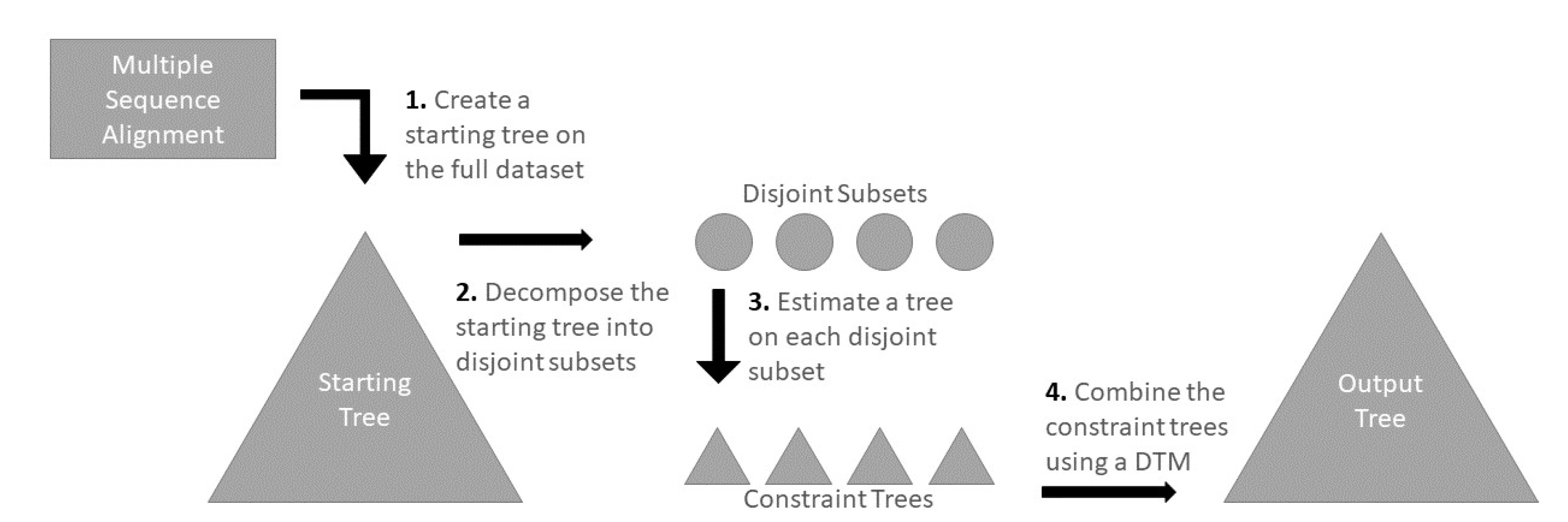
Figure 1 describes the DTM pipeline.
We used simulated datasets to evaluate phylogeny estimation methods, so that the true alignment and true tree are known. In each case, we provided the true alignment to the different methods and recorded the tree error as well as the running time. Our simulated datasets come from five model conditions and they range in terms of size and difficulty. One of these model conditions evolved under the standard i.i.d. Generalized Time Reversible (GTR) model equipped with insertions and deletions, but others evolved under models with additional complexity (e.g., heterotachy across the gene and across the tree, or under a model that includes selection). We also specifically explored a model condition that contains fragmentary sequences (e.g., a case that arises in real biological analyses when combining full-length sequences with reads or partially assembled sequences as a result of using high-throughput sequencing technologies).
We performed three experiments. The initial experiment was performed on just one model condition to determine (a) how we would define distances for use within two of the DTM pipelines that require guide distance matrices and (b) the maximum subset size for the decomposition. The second experiment was performed on three model conditions with 1000 to 2341 sequences to evaluate the impact of the starting tree on DTM pipelines and compare them to the three ML heuristics that we selected. Our third experiment evaluated the two faster pipelines with respect to the speed and accuracy on datasets with 10K and 50K sequences, and then compared them to the three ML heuristics that we selected.

2.2. Methods

2.2.1. Maximum Likelihood Codes

We use three existing codes for maximum likelihood (ML): FastTree 2, RAxML-NG, and IQ-TREE 2; for the sake of simplicity, we will subsequently refer to these methods as FastTree, RAxML, and IQ-TREE. All of these methods are run under the GTR+G (i.e., GTR with gamma-distributed rates across sites) model of evolution.
FastTree does not make a strong attempt to find the best solution to ML and, instead, stops the search (using nearest neighbor interchange, or NNI, moves) after a polynomial number of moves. This approach makes it faster than the other methods, which continue searching until there is evidence of having found a good local optimum. Moreover, in our study, FastTree completed on all datasets. The other methods did not complete on some of the datasets within the allowed run-time limit (24 h for the datasets with at most 2341 sequences, and one week for the datasets with 10K or 50K sequences), using the available memory (generally limited to 64 Gb). In such cases, we used the best tree (i.e., the tree with the best ML score, according to the code) found for that method on that dataset.

2.2.2. Disjoint Tree Mergers Pipelines

Given an input dataset (here, a multiple sequence alignment), a DTM pipeline has four steps:
  • Step 1: compute a starting tree
  • Step 2: use the starting tree to decompose the set of sequences into disjoint sets
  • Step 3: construct the trees on the different sets using a selected phylogeny estimation method, and
  • Step 4: merge the trees using a DTM method along with some auxiliary information (e.g., guide tree or distance matrix)
Thus, Step 4 is where the DTM method is used. We begin by describing how TreeMerge, Constrained-INC, and GTM operate at a very high level, and then describe how they are used in divide-and-conquer pipelines.
The input to each DTM is a set of disjoint subset trees, which are treated as constraint trees, as well as some auxiliary information. For the purpose of this study, each DTM is able to use the starting tree for its auxiliary information, and so we describe these methods with that modification.

2.2.3. TreeMerge

TreeMerge takes as input the set of k disjoint trees and a guide tree, and the guide tree is used to compute a matrix of leaf-to-leaf distances. TreeMerge then operates in two stages, where the first stage produces a set of k 1 pairwise merged constraint trees, and the second stage merges these k 1 constraint trees into a tree on the full dataset. The first stage is operated, as follows. First, a spanning tree on the input constraint trees is computed using the distance matrix, and the edges of the spanning tree then define which pairs of constraint trees will merged into larger (and now overlapping) trees. These overlapping pairs are then merged together using NJMerge, while using the provided or computed distance matrix. Note that NJMerge allows for the full blending of two trees. In Stage 2, the larger constraint trees are combined, two at a time, until all of the larger constraint trees are merged together, which results in a tree on the full dataset that is compatible with all of the original input constraint trees. To merge two trees that overlap, TreeMerge computes the branch lengths on the trees and then uses these branch lengths to determine how to merge the trees on the region in which they overlap. This step allows for a partial, but not full, blending (see [20] for full details). We also made a small modification to the TreeMerge approach. Specifically, we discovered that the technique that was used by TreeMerge (i.e., PAUP*) to compute branch lengths in order to merge overlapping trees was a computationally expensive step. We evaluated the use of RAxML instead of PAUP* for this branch length estimation and found it reduced the running time without changing accuracy (see Table A2). Hence, we made this modification in our TreeMerge analyses.

2.2.4. Constrained-INC

Constrained-INC takes as input the set of disjoint constraint trees and a starting tree, and it incrementally builds a tree that obeys the constraint trees by (a) computing a distance matrix from the starting tree and (b) computing quartet trees that will vote on where to place each species into the growing tree. Although the set of quartet trees Constrained-INC uses can be estimated from a distance matrix or by recomputing quartet trees using an ML method, better accuracy is obtained using induced quartet trees from a starting tree estimated using an ML heuristic [24], and so we describe the algorithm in this context. Constrained-INC operates by building a tree that obeys the constraint trees by incrementally adding the species, one-by-one, using a distance matrix (which, in our study, is computed from the starting tree). To place a new species into the tree, it uses selected quartet trees that are defined by the starting tree, with a voting scheme that weights the quartet trees using the distance matrix. The final tree is returned once all of the species are included. Each placement is guaranteed to obey the constraint trees, so that the final tree is guaranteed to obey the constraint trees. By design, Constrained-INC (where “INC” refers to incremental) allows full blending.

2.2.5. Guide Tree Merger (GTM)

The input to GTM is a set of constraint trees and a guide tree (in this study, we use the starting tree as the guide tree to GTM). GTM constructs a tree on the full set of species by adding edges between the constraint trees; hence, GTM does not allow any blending. Furthermore, GTM returns a tree T that is guaranteed to minimize the total Robinson–Foulds distance to the guide tree, and it does so in polynomial time.

2.2.6. Steps 1–3 Pipeline Details

To complete the description of the existing DTM pipelines we explore, we now describe Steps 1–3. In Step 1, an initial tree is computed on the alignment using an existing maximum likelihood (ML) tree estimation method. In Step 2, the starting tree is decomposed into subtrees by repeatedly removing centroid edges (i.e., edges that decompose the tree roughly equally into two parts) until the size of each subtree is below a user-specified maximum subset size (this is the same decomposition as used in several multiple sequence alignment methods, including SATé-II [27], PASTA [28], and MAGUS [29]). The leaves in each subtree define a subset of the sequences in the input sequence alignment, and a ML tree is computed on each subset of sequences using the ML method (Step 3). Finally, in Step 4, these subtrees are merged together using the selected DTM method (i.e., TreeMerge, GTM, or Constrained-INC). These DTM methods require auxiliary information, with TreeMerge requiring a distance matrix, GTM requiring a guide tree, and Constrained-INC requiring either a distance matrix or a guide tree that can be used for defining the distance matrix.
For this study, the starting trees are computed using IQ-TREE or FastTree, we decompose these starting trees using the centroid decomposition with varying maximum subset size, and the subset trees are computed using IQ-TREE. We use the starting tree from Step 1 for the guide trees.

2.3. Datasets

Our datasets range in size from 1000 to 50,000 sequences, and they vary in complexity and difficulty; see Table 2. The RNASim datasets evolve under a model that incorporates fitness and positive selection to maintain the RNA structure [28], and so evolve under a non-i.i.d. model. The Cox1-HET dataset evolves with heterotachy across the tree, and it was created for this study. The 1000M1-HF datasets evolve under a standard GTR substitution model with indels, and have a high rate of evolution, and some of the sequences are fragmentary; this makes the inference of the tree challenging for these datasets. In each case, we use the true alignment as input to the tree estimation method. Note that only one of the model conditions that we explore (1000M1-HF) evolves under a standard GTR+indel model. By including models that incorporate selection or variability of the model process across the tree as well as across the sites, we have expanded the model space to incorporate more biological realism.
  • 1000M1-HF. These 1000-sequence datasets are from a prior study [16], where half of the sequences have been fragmentary. We picked the first five replicates only.
  • RNASim1000. We sampled five 1000-sequence subsets of the single million-sequence replicate from the RNASim million-sequence dataset studied in [28].
  • Cox1-HET. This is a dataset developed explicitly for this study containing 2341 sequences, and described in detail below. We created 10 replicates.
  • RNASim10K. We sampled 10,000-sequence subsets of the RNASim million-sequence datasets (ten replicates).
  • RNASim50K. We used the same strategy as for the RNASim10K analysis but sampled 50,000-sequence subsets (ten replicates).

2.3.1. 1000M1-HF

This dataset was used in [16], and it was created by fragmenting half of the sequences in each replicate of the 1000M1 model condition from [30], making each fragmentary sequence 25% of the original median sequence length. The reference trees provided with this dataset are the “potentially inferrable model trees”, which means that the zero-event branches (i.e., branches on which no substitution or indel occurs) are collapsed, hence creating a non-binary reference tree. This dataset is publicly available, and we use the first five replicates from this collection.

2.3.2. RNASim1000

RNASim1000 was created for this study by randomly sampling five subsets with 1000 sequences each from the single million-sequence replicate of the RNASim dataset used in [28] to evaluate multiple sequence alignment methods. Once the sequences were sampled, the reference trees were induced from the original RNASim million-sequence reference tree on the same set of taxa that the sequences represent. Appendix C provides the code used to generate these sequences.

2.3.3. Cox1-HET

We created a dataset for which the sequences would evolve under different model parameters across the tree, in order to evaluate tree estimation methods in the presence of heterotachy [31]. We began by estimating a species-level biological cox1 barcode gene tree (see Appendix B). The tree of 2341 species was decomposed into 324 subtrees using centroid edge decomposition, with maximum subset size 10, using the decompose.py script (see Appendix C). For each of the 324 subsets, we estimated the numeric GTR+G parameters using IQ-TREE v1.6.12. Each set of numeric model parameters (i.e., substitution rate matrix, stationary frequencies, and discrete gamma model) was then assigned to the corresponding subset in the model tree following the INDELible format [32]. Subsequently, we used INDELible V1.03 [33] to simulate new sequences down the model tree (with 324 different model parameters). Because the proportion of invariant sites cannot be changed across the tree in INDELible V1.03, we fixed this proportion at 15.78%, the overall proportion of invariant sites in the original sequence dataset. We repeated the sequence evolution for 10 replicates, and name this dataset “Cox1-HET”.

2.3.4. RNASim10K

We took the first ten trials of the million-sequence RNASim dataset from [34] and randomly extracted a sub-sample of 10,000 for each trial. The result is a dataset of 10 replicates of 10,000 sequences. Once the sequences were sampled, the reference trees were induced from the original RNASim million-sequence reference tree on the same set of taxa that the sequences represent.

2.3.5. RNASim50K

We used the same procedure as for the RNASim10K dataset, but sampled subsets with 50,000 sequences, producing 10 replicate datasets.

2.4. Computational Platform

Most of the analyses were run on the Illinois Campus Cluster, with the exception of the TreeMerge analyses on the Cox1-HET dataset as well as the RNASim10k and RNASim50k datasets, which were run on NCSA’s Blue Waters. All of the analyses were allowed between 54 Gb and 64 Gb of memory, an amount that is sufficient for all alignments of the sizes that we study, with the exception of one model conditions which involves 50,000 sequences. Unless otherwise specified, no method came close to being bottlenecked by the limitations on allocated memory.
Most of the multi-threaded methods were allowed between 10 and 16 cores, with few exceptions. Each constraint tree estimation for the 1000M1-HF and RNASim1000 datasets was allowed to run with up to four cores, with IQ-TREE deciding the appropriate number of cores. For the Cox1-HET dataset, constraint trees estimated with IQ-TREE were allowed to run up to 16 cores, and we let IQ-TREE select the appropriate number of cores; most of the constraint tree calculations only used 1–3 cores.
Constrained-INC and GTM were used in their currently available implementations, taken from the developers’ Github repositories, and are single-threaded. TreeMerge was modified to take in pre-estimated RAxML branch lengths (that were computed with two cores), and is otherwise run single-threaded.

2.5. Evaluation Criteria

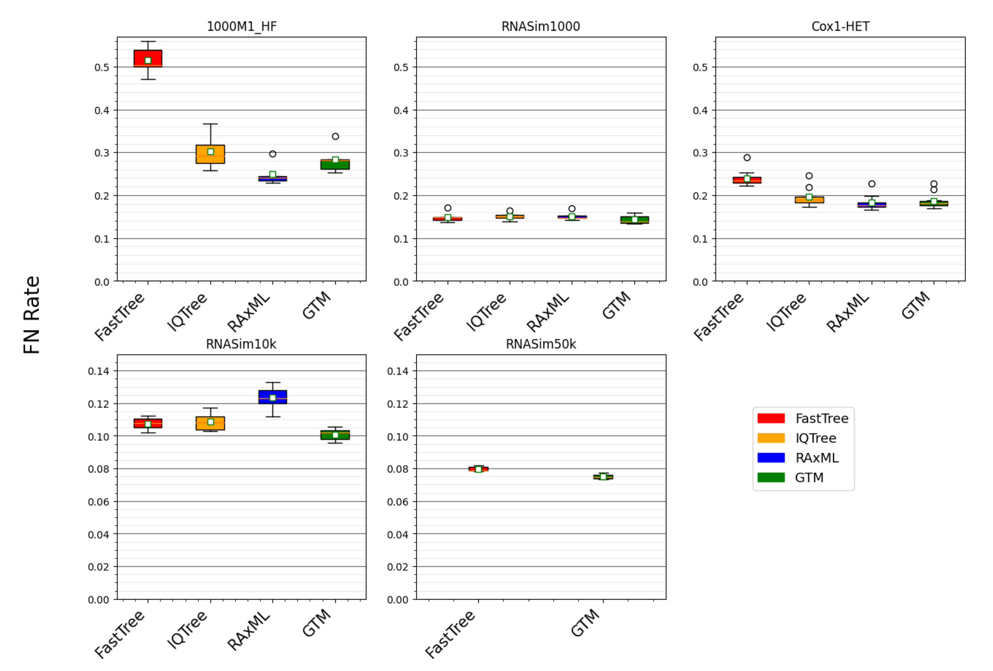
Our focus is on the topological error in the estimated tree in comparison to the reference tree for the simulation study. Every tree t can be represented by its set π ( t ) of edge-induced bipartitions; hence, the set π ( T ) π ( t ) , where t is the estimated tree and T is the true tree, is the set of “missing branches” or “false negatives”. Conversely, the set of false positives is π ( t ) π ( T ) . The false negative (FN) rate is the number of false negatives divided by the number of internal branches in the true tree, and the false positive (FP) rate is the number of false positives divided by the number of internal edges in the estimated tree. These rates are identical when the estimated and true tree are both fully resolved (i.e., binary), in which case they are also equal to the commonly used Robinson–Foulds (RF) error rate.
1000M1-HF is the only model condition we explore that has non-binary reference trees, where the reference trees are about 0.4% unresolved (Table A1); all other model conditions have binary reference trees. In addition, all of the estimated trees are also binary. Hence, for the model conditions other than the 1000M1-HF condition, the RF error rate is exactly the same as the FN error rate. We report FN rates for all methods here, and note that the difference between FP and FN rates on the 1000M1-HF datasets is approximately 0.3%. To compute these error rates, we use a script that was coded by Erin K. Molloy (see Appendix C).
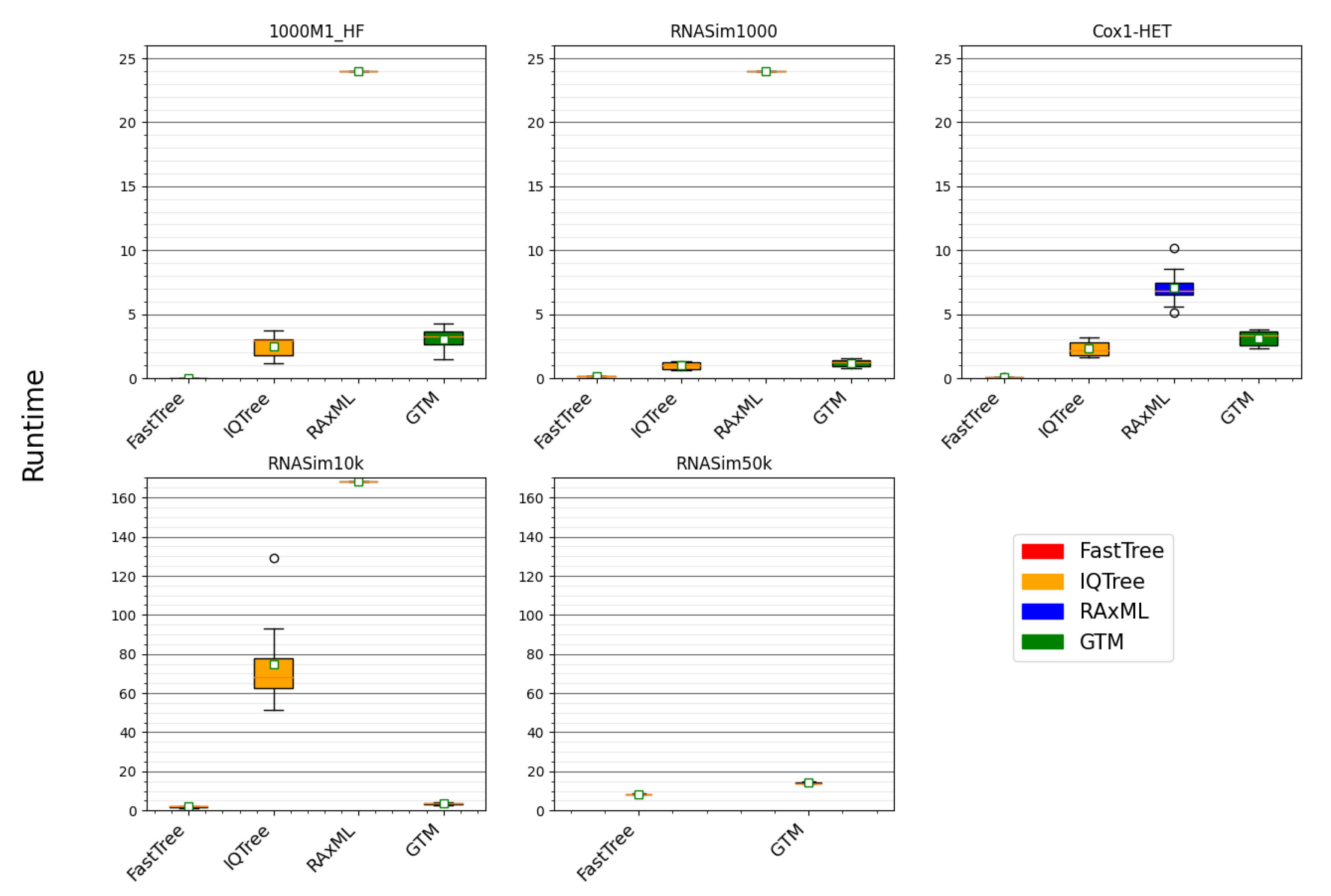
We also evaluate methods with respect to running time. In all of our analyses, we assume a maximum of 16 core parallelism, i.e., when running constraint tree calculations in parallel, only those analyses that will fit under 16 cores are considered to be parallel, assuming that a typical computational platform would have access to 16 cores. In cases where multiple methods are used in stages, such as the DTM pipelines, the same assumption of 16 core parallelism applies. In a DTM pipeline, the run-time calculation is the sum of running times of computing the starting tree, constraint trees, and the running time of disjoint tree merger. No given method or a set of methods running in parallel was allowed to use more than 16 cores.

3. Results

3.1. Experiment 1: Evaluating the Impact of Distance Matrix Calculation and Subset Size on DTM Pipelines

In this experiment, we evaluated variants of how the distance matrix is computed, using the Cox1-HET model condition, to see whether these resulted in any improvements in running time and accuracy. These different distances were computed from the input sequence alignments using several techniques that are available in FastME [35] (including under different sequence evolution models) as well as using leaf-to-leaf distances within the guide tree (either topological distances or taking branch lengths into account). In these analyses, using distances computed from the guide tree resulted in more accurate trees than when using distances computed directly from the sequence alignment (Table A3). Furthermore, when computing distances using the guide tree, it was either neutral or beneficial to use topological distances instead of distances that are based on branch lengths (Table A3 and Table A4).
We also evaluated the impact of varying the maximum subset size in the decomposition used with Constrained-INC and GTM. We found that larger subsets improved accuracy, with substantial improvements as the subset sizes increased from 20 up to 500 (Table A3Table A5). We also found that trees based on maximum subset size 1000 were not more accurate than trees computed using maximum subset size 500 (Table A5).
Based on these initial evaluations, in our subsequent experiments we set the maximum subset size to 500 and used topological distances that were computed from the starting tree (which we also used as a guide tree) in TreeMerge and Constrained-INC.

3.2. Experiment 2: Evaluating the Impact of the StartingTree on DTM Pipelines

We evaluated the different DTM pipelines in comparison to the three ML methods, using datasets with 1000 to 2341 sequences; the trends described below are based on Table 3, Table 4 and Table 5, with specific examples or exceptions as indicated.
  • A comparison of the three ML heuristics shows that RAxML generally produces the most accurate trees, followed by IQ-TREE, and then by FastTree; the exception is the RNASim1000 condition where all three methods obtain about the same accuracy and FastTree is slightly more accurate than the other methods (Table 3). In the model conditions without fragmentary sequences, IQ-TREE and RAxML were very close in accuracy (Table 3 and Table 4), but RAxML was clearly more accurate than IQ-TREE on the fragmentary model condition (Table 5). FastTree had particularly poor accuracy on fragmentary sequences, but it was also clearly less accurate than the other methods on the model condition with heterotachy (Table 4). RAxML is the slowest and FastTree is the fastest.
  • For each DTM method, using IQ-TREE instead of FastTree for the starting tree nearly always improved the accuracy. The one case where we did not see this trend was for the Cox1-HET, where, using Constrained-INC with the FastTree starting tree, was slightly better than using the IQ-TREE starting tree (Table 4).
  • The DTM methods produced trees with similar accuracy, with a small disadvantage to Constrained-INC when using the IQ-TREE starting tree.
  • When using an IQ-TREE starting tree, most of the time in using a DTM pipeline was spent constructing the starting tree. Furthermore, the DTM methods are very fast when using FastTree starting trees and slower when using IQ-TREE starting trees (and, by design, the DTM methods must be slower than their starting trees). Finally, TreeMerge was slower than the other DTM methods. (These observations are based on comparing running times for DTM pipelines to the starting tree runtimes.)
  • For every model condition, the TreeMerge and GTM pipelines produced more accurate trees than their starting trees, but the improvement was small for IQ-TREE starting trees (0.7% to 1.8%) and varied for FastTree starting trees (0.2% to 8.5%).
  • For every model condition, the TreeMerge and GTM pipelines using IQ-TREE starting trees matched or improved both FastTree and IQ-TREE with respect to accuracy, with the improvement in accuracy, depending on the model condition (and ranging from 0.7% to 1.8%).
  • The differences in accuracy using GTM or TreeMerge pipelines with FastTree or IQ-TREE starting trees were small (at most 0.3% in Table 3 and Table 4), with the exception of the 1000M1-HF datasets, where the difference was large (14.1% in Table 5). Hence, the choice of starting tree can matter for some model conditions.
  • No DTM pipeline was consistently able to match the accuracy of RAxML. That is, for one model condition (RNASim1000), all of the DTM pipelines matched or improved on RAxML, but no DTM pipeline matched RAxML on the other two model conditions (Table 3). The difference in accuracy between RAxML and the GTM or TreeMerge pipelines using IQ-TREE starting trees was 0.5% for the Cox1-HET dataset and 3.5% for the 1000M1-HF datasets (Table 4 and Table 5).
  • RAxML had a higher running time than these DTM pipelines, especially when the GTM pipeline is used. For example, the GTM pipeline completed in 1.2 h on the RNASim1000 datasets, 3.1 h on the Cox1-HET datasets, and 3.1 h on the 1000M1-HF datasets, whereas RAxML did not complete within 24 h on two of the model conditions and only completed in 7.1 h on the Cox1-HET datasets.
In summary, the generally most accurate DTM pipelines are based on GTM or TreeMerge, and use IQ-TREE starting trees, decomposition size 500, and IQ-TREE constraint trees. These DTM pipelines provide an advantage over FastTree and IQ-TREE for accuracy, but they do not reliably provide an advantage over RAxML. GTM has an advantage over the other two DTM methods (running time advantage over both, and slight accuracy advantage over Constrained-INC). Hence, the benefit in terms of accuracy in using these pipelines is limited if the dataset is small enough for RAxML to be used, and these pipelines are always slower than IQ-TREE.

3.3. Experiment 3: Evaluating Fast DTM Pipelines in Comparison to ML Codes on Ultra-Large Datasets

Because TreeMerge did not offer an accuracy advantage over GTM and it is slower than GTM and Constrained-INC, for our experiment evaluating scalability to 10K and 50K sequences, we only examined the DTM pipelines using GTM and Constrained-INC. We compared these two pipelines (using the same starting tree and decomposition strategy) to all three ML methods, allowing all methods up to one week of running time, given 16 cores and using 64GB of memory. Table 6 and Table 7 show results on the RNASim10K and RNASim50K datasets, respectively, and are separately discussed.
On the RNASim10K datasets (Table 6), FastTree completed in two hours, IQ-TREE completed in just under 75 h, and RAxML did not complete within the allowed running time (one week). We report the FN error rate for the best ML tree that was found by RAxML before it timed out. The comparison between the three ML methods shows that FastTree and IQ-TREE are tied for the best accuracy (10.8% and 10.9% error, respectively), followed by RAxML at 12.3%. The GTM pipeline achieves 10.1% error and the Constrained-INC pipeline achieves 10.5% error, and both complete quickly (3.5 h for GTM and 4.3 h for Constrained-INC). Thus, on these datasets, the two DTM pipelines are more accurate than all of the ML methods tested and are also much faster than either IQ-TREE or RAxML.
The results on the RNASim50K datasets (Table 7) are somewhat different. First, IQ-TREE fails to return a tree (failing due to a memory allocation problem) and, while RAxML does not fail, the tree it returns has 100% topological error. FastTree, as before, achieved good accuracy, with an error rate of 8.0%, and it does so in just 8.3 h. The GTM pipeline also completed and returned a tree with good accuracy (7.5% error), improving on the FastTree starting tree, and it did so in 14.1 h. However, Constrained-INC failed to return a tree on these datasets due to a memory allocation problem.
Thus, for these two model conditions with RNASim10K and RNASim50K sequences, the GTM pipeline is faster, manages limited memory conditions better, and produces better accuracy than the Constrained-INC pipeline. The comparison between the ML heuristics (IQ-TREE, RAxML, and FastTree) shows that FastTree can have better accuracy than the other two methods, and it also reveals challenges for IQ-TREE to successfully run on the RNASim50K dataset.

Summary of Observed Trends

The DTM pipeline that had the best accuracy used IQ-TREE as the starting (and guide) tree as well as for the constraint trees, and then combined the constraint trees using GTM. However, IQ-TREE could not be used to compute the starting tree on the RNASim50k datasets, and it was computationally intensive on the RNASim10k datasets. Therefore, we use FastTree for the starting and guide tree on the datasets with 10,000 or more sequences.
The comparison between this GTM pipeline and the ML heuristics (RAxML, FastTree, and IQ-TREE), shown in Figure 2 (error rates) and Figure 3 (running time), show that the GTM pipeline is competitive with the best of the ML heuristics for accuracy. GTM always matches or improves on IQ-TREE and FastTree for accuracy and, although RAxML is more accurate than the GTM pipeline on the 1000M1-HF dataset, GTM either matches RAxML’s accuracy or improves on it on the other datasets.
Thus, overall, the GTM pipeline provides accuracy that is competitive with the best competing methods, and it is (with FastTree) the only method in this collection that was able to run within the time limit provided on the largest dataset. Furthermore, GTM is just slightly slower than its starting tree, making it feasible to use GTM even on very large datasets, since FastTree is generally able to run on even ultra-large datasets.

4. Discussion

This study provides some insights into the conditions that impact the relative accuracy and running times of three leading maximum likelihood (ML) codes, and into the potential for Disjoint Tree Merger (DTM) pipelines to provide improved accuracy and/or scalability when compared to these ML codes. Our simulation included some model conditions that were relatively “easy” (i.e., the RNASim1000 condition) and then model conditions that were more challenging due to the inclusion of fragmentary sequences (i.e., the 1000M1-HF condition), heterotachous sequence evolution model (i.e., Cox1-HET), or very large or ultra-large datasets (i.e., RNASim10K and RNASim50K, respectively).
Our study showed differences between the basic ML heuristics—RAxML, IQ-TREE, and FastTree—that depended, in part, on the dataset size and properties, as well as between the different DTM pipelines. However, the main focus of this study was to determine whether any of the current DTM pipelines provide improved accuracy over the better ML codes in the context of gene tree estimation. Hence, we begin by discussing what we learned about the differences between the three ML codes.

4.1. Comparison of the Three ML Codes

The running time comparison shows RAxML to be clearly the most computationally intensive, followed by IQ-TREE, and then by FastTree, which is, by far, the fastest method. Therefore, we begin by comparing FastTree to the other methods (Figure 3). On two conditions (i.e., RNASim1000 and RNASim10k datasets), FastTree ties for best among these methods (Table 3 and Table 6). However, on the datasets with fragmentary sequences (1000M1-HF) or with heterotachy (Cox1-HET), FastTree is clearly less accurate than both RAxML and IQ-TREE (Table 4 and Table 5). Hence, FastTree, although, by far, the fastest of these methods, is less robust to these challenging conditions.
A comparison between RAxML and IQ-TREE is also interesting. RAxML and IQ-TREE have nearly identical accuracy on RNASim1000, and there is only a small advantage to RAxML on the Cox1-HET datasets (Table 3 and Table 4). However, RAxML is much more accurate than IQ-TREE on the 1000M1-HF dataset, and it is much less accurate on the RNASim10k dataset (Table 5 and Table 6). Hence, the relative performance of RAxML and IQ-TREE depends on the dataset properties, with size and sequence length heterogeneity distinguishing the two methods.
This study shows that very large datasets present specific challenges to ML heuristics. On the RNASim10K dataset, all of the tested methods were able to return reasonably accurate trees within the limitations on running time and available memory, but the same did not hold for the RNASim50K dataset (Table 6 and Table 7). This trend suggests that algorithmic strategies for ML heuristics that have been successful on smaller datasets (with at most 1000 or so sequences) may be counterproductive on ultra-large datasets. Specifically, when the sequence dataset is ultra-large, with many thousands (or tens of thousands) of sequences, methods, such as RAxML and IQ-TREE, which make a significant effort to produce good likelihood scores through numeric parameter optimization may not be competitive (in terms of topological accuracy) with methods (such as FastTree) that do not make as serious an effort to optimize the numeric parameters and, instead, focus on exploring more model tree topologies.

4.2. Comparison between DTM Pipelines

Our study showed that the algorithmic choices within the DTM pipelines (starting tree, maximum subset size, and how the distance matrix is computed for use with Constrained-INC and TreeMerge) impact accuracy. In general, we found that using a highly accurate starting tree and larger maximum subset sizes, as well as computing the distance matrix using topological distances, produces better final topological accuracy when compared to the alternative variants of DTM pipelines that we tested. The first two observations (impact of starting tree and subset size) were also noted in [24], but using a different set of options for each algorithmic step. Our third observation, that using topological distances in the guide tree instead of other ways of defining pairwise distances of sequences (for use within Constrained-INC or TreeMerge) is beneficial, has not been communicated in any prior publication in the context of gene tree estimation; however, similar findings were reported in the context of species tree estimation in [25].
One of the surprising findings in this study is that we did not see substantial differences in accuracy in the trees that were computed using our better pipelines once everything other than the DTM method (Constrained-INC, TreeMerge, or GTM) is fixed. This is interesting since the DTM methods use very different strategies for merging disjoint subtrees, especially with respect to the degree of blending that is permitted. Specifically, GTM does not allow any blending, TreeMerge allows partial blending, and only Constrained-INC allows full blending. Given the close accuracy between the DTM pipelines, computational issues become important and, thus, pipelines using GTM are superior to the other DTM pipelines, which are slower.
Another trend observed in this study is that DTM pipelines are impacted (even if only by a small amount) by the choice of the starting tree. The impact of a poor decomposition on GTM makes sense, since, if the subsets are not convex in the true tree (i.e., separable from each other by edge deletions), then the requirement to not blend subset trees means that the true tree cannot be constructed using GTM. Therefore, it is noteworthy that the other DTM methods, which do allow blending, are also negatively impacted by poor starting trees.

4.3. Comparing DTM Pipelines to ML Heuristics

Our study showed that the best DTM pipelines we explored (which use IQ-TREE starting and constraint trees) provide improved accuracy as compared to both FastTree and IQ-TREE, but they are not as reliably accurate as RAxML, a finding that should be contrasted with the trends (and interpretation) reported in the prior study evaluating Constrained-INC pipelines for gene tree estimation [24]. It is worth noting that [24] never found their best pipeline using Constrained-INC to be competitive with RAxML and, indeed, their pipelines were not reliably more accurate than FastTree. This is very different from what we observe, where the best GTM pipeline is reliably more accurate than FastTree and IQ-TREE and, in some cases, as accurate as RAxML (or even more accurate than RAxML).
The difference in trends can be explained by the choices made in [24] for the Constrained-INC pipeline, which—in many cases—reduced accuracy when compared to the choices that we made. Of the many differences, the three most likely to have negatively impacted the Constrained-INC pipeline in [24] as compared to the better pipelines that we studied are (1) the use of Constrained-INC instead of GTM, (2) the smaller maximum subset size (they used 200) compared to ours (we used 500), and (3) the use of FastTree instead of IQ-TREE as the starting tree in all analyses. Thus, the choice of algorithmic parameters has a substantial impact on pipeline accuracy, and our choices improved accuracy when compared to theirs.
Thus, unlike [24], we find that the better DTM pipelines can provide competitive accuracy with leading ML heuristics. Moreover, the best DTM pipeline that we developed—GTM using IQ-TREE for starting tree and constraint trees–was competitive with RAxML, and only clearly less accurate than RAxML on the high fragmentary 1000M1-HF condition. Furthermore, for that high fragmentary condition, the problem was that the starting tree (that was produced using IQ-TREE) had high error—30.2%. The GTM pipeline reduced this error by 1.8%, but this was not enough to come close to RAxML, which had error of only 24.9%. In other words, the GTM pipeline that we presented was only able to reduce the error over the starting tree by a small amount, and when the gap in accuracy between the starting tree and RAxML is large; this means that the pipeline will not be competitive with RAxML.
This examination reveals that DTM pipelines can be competitive with RAxML in accuracy (and much faster) when IQ-TREE or FastTree can produce a tree that is close to the accuracy of the RAxML tree. However, as the high fragmentary condition (1000M1-HF) shows that there are conditions where neither FastTree nor IQ-TREE are nearly as accurate as RAxML. For such cases, DTM pipelines will fail to be competitive in terms of accuracy with RAxML.

4.4. Limitations of This Study

This study was limited to only a few model conditions (and, further, three of the five model conditions are based on subsets of the RNASim million-sequence simulation), and so trends observed here may not hold under very different conditions. In particular, the relative performance between methods may be very different for much smaller datasets (where optimizing the ML may be achieved well by some methods) or on much larger datasets. In particular, if the running time and available memory are limited, then it may be that only FastTree will be able to analyze very large datasets, and both IQ-TREE and RAxML will be infeasible. Another trend we saw that may not hold under other conditions is that pipelines using GTM were as accurate as the pipelines using TreeMerge or Constrained-INC; it is possible that other conditions will be found where GTM is not as accurate as TreeMerge or Constrained-INC, due to GTM’s inability to blend its constraint trees.

4.5. Future Work

This study suggests several directions for future work. First, to design a DTM pipeline that has the potential to consistently and reliably match or improve on the accuracy of RAxML, it will be necessary to change the DTM pipeline. One possibility is to change how we obtain the initial decomposition. Using a good starting tree is obviously desirable, but, as RAxML is very expensive, this is not computationally feasible on large datasets. Instead, other techniques for decomposing the input dataset should be considered, including fast clustering methods or sequence similarity based decompositions. A second change that might improve accuracy is to use RAxML instead of IQ-TREE to compute the constraint trees. However, that substitution in the pipeline design would increase the running time, as RAxML is significantly more expensive than IQ-TREE.
This study is also suggestive of other directions for improving large-scale phylogeny estimation. For example, the results that are shown here suggest that iteration might result in improved accuracy, since the DTM pipelines that we presented reliably improved on their starting trees. Divide-and-conquer pipelines are embarrassingly parallel due to the fact that the constraint trees on the disjoint subsets can be computed independently. Hence, a natural direction for future work in terms of runtime gain is a careful parallel implementation of these pipelines, in order to achieve improved wall-clock running times when compared to existing approaches.
Finally, evaluating ML methods for gene tree estimation presents specific challenges, especially when topological accuracy is the main objective. Benchmark biological datasets where the true gene tree is known (or where at least most of the branches are reliably known) would be helpful, but, since gene tree discord with the species tree is a common and well established phenomenon [22], relying on comparisons to the species tree (which itself may not be known with high reliability) is not an acceptable substitute. Alternatively, developing additional large-scale single gene simulations that are biologically realistic and, hence, can be used to characterize method performance would be useful.

5. Conclusions

This study provides new insight into maximum likelihood (ML) tree estimation on large gene sequence datasets. We compared three leading ML heuristics—RAxML-NG, IQ-TREE 2, and FastTree 2—on five different model conditions with 1000 or more sequences with respect to the topological accuracy and running time. We found that RAxML-NG and IQ-TREE 2 were more robust to challenging conditions that were characterized by sequence length heterogeneity and substantial heterotachy than FastTree 2. We also observed that RAxML-NG was the most computationally intensive of the three ML methods and FastTree 2 was the fastest. The comparison between RAxML-NG and IQ-TREE 2 showed that they had similar accuracy under some conditions, but RAxML-NG was more accurate on the datasets with fragmentary conditions (thus displaying greater robustness to this challenging condition than IQ-TREE 2), but less accurate on the RNASim10K datasets. Thus, the choice between RAxML-NG and IQ-TREE 2 may depend on the dataset size (with IQ-TREE 2 being preferred for the largest datasets), as well as the available computational resources. Moreover, our study suggests that gene tree maximum likelihood estimation using RAxML-NG is not likely to be feasible for the very large datasets.
Our study then explored the design space for divide-and-conquer pipelines using three DTM methods. In contrast to an earlier study [24], which found that a divide-and-conquer pipeline using Constrained-INC did not provide an advantage over its starting tree for gene tree estimation, our new pipeline reliably produces trees more accurately than both IQ-TREE 2 and FastTree 2 starting trees. However, we also saw that, to consistently match or improve on of RAxML-NG while being substantially faster, will require changes to the current divide-and-conquer strategy and most likely will require a new approach to decomposing the input set of sequences into disjoint sets that is fast and suitable for subsequent use in a DTM pipeline.
Although this study was only based on a few model conditions and much work is still needed to understand the relative performance of different methods and the conditions under which each method is generally reliable, this study suggests the following guidelines for the selection of ML heuristic:
  • When the dataset sizes and computational resources make it feasible to use RAxML-NG or IQ-TREE 2, these methods should be used rather than FastTree 2, due to their (generally) higher level of topological accuracy when analyzing datasets that evolve under non-i.i.d. models (which may be typical of biological datasets). The choice between IQ-TREE 2 and RAxML-NG is less clear, as the relative accuracy of these two methods depended on the model condition. However, when datasets have substantial numbers of fragmentary sequences, RAxML-NG may be preferable to IQ-TREE 2.
  • For very large datasets where RAxML-NG and IQ-TREE 2 are not feasible to run, then FastTree 2 or one of the DTM pipelines that we presented could provide reasonable accuracy.
In summary, this study is very positive with respect to the potential for DTM pipelines to improve the scalability of gene tree estimation. First, the current best DTM pipeline improves on IQ-TREE 2 and FastTree 2, which had not been seen before. Second, we have identified an algorithmic challenge—the fast and accurate clustering of sequence datasets—that may provide the key to improving the DTM pipeline accuracy and scalability to large and more challenging datasets. Advances on this basic challenge could lead to substantial breakthroughs for large-scale phylogeny estimation. This study also showed that the phylogenetic estimation error rates can decrease with increased taxonomic sampling (a trend that has been observed in other studies [13]), provided that good tree estimation methods are used, showing the value of developing methods that can scale well to large datasets. Overall, therefore, this study suggests new designs for large-scale phylogeny estimation that have both high accuracy and speed.

Author Contributions

Conceptualization, M.P., P.Z. and T.W.; methodology, M.P., P.Z. and T.W.; software, M.P.; validation, M.P.; investigation, M.P.; writing—original draft preparation, T.W.; writing—review and editing, M.P., P.Z. and T.W.; supervision: P.Z. and T.W.; funding acquisition, T.W. All authors have read and agreed to the published version of the manuscript.

Funding

This research was funded in part by US National Science Foundation grant number NSF DBI 14-58652 (to T.W.).

Institutional Review Board Statement

Not applicable.

Informed Consent Statement

Not applicable.

Data Availability Statement

The codes necessary to perform the experiments are available in public databases, and these locations are provided in the Appendix C. Most of the datasets were used in prior published studies, and hence available in public repositories (see text). Those datasets generated specifically for this study, the trees estimated on the datasets, and the information necessary to reproduce the Cox1-HET simulation are available on the Illinois Data Bank at https://doi.org/10.13012/B2IDB-7008049_V1 (accessed on 5 May 2021).

Acknowledgments

We thank Thien Le for assistance with the Constrained-INC code. We would also like to thank Nicolas Puillandre for providing us a curated list of cox1 GenBank identifiers for Neogastropoda. This work made use of the Illinois Campus Cluster, a computing resource that is operated by the Illinois Campus Cluster Program (ICCP) in conjunction with the National Center for Supercomputing Applications (NCSA) and which is supported by funds from the University of Illinois at Urbana-Champaign. This research is part of the Blue Waters sustained-petascale computing project, which is supported by the National Science Foundation (awards OCI-0725070 and ACI-1238993) the State of Illinois, and as of December 2019, the National Geospatial-Intelligence Agency. Blue Waters is a joint effort of the University of Illinois at Urbana-Champaign and its National Center for Supercomputing Applications.

Conflicts of Interest

The authors declare no conflict of interest. The funders had no role in the design of the study; in the collection, analyses, or interpretation of data; in the writing of the manuscript, or in the decision to publish the results.

Abbreviations

The following abbreviations are used in this manuscript:
DTMDisjoint Tree Merger
GTMGuide Tree Merger
GTRGeneralized Time Reversible
GTR+GGTR model with Gamma-distributed rate variation among sites
MLMaximum Likelihood

Appendix A. Additional Tables

Table A1. 1000M1 Resolution. Here, e 1 is the number of internal edges in the “PIMT”, or the Potentially Inferrable Model Tree, where the zero-event edges are collapsed, and e 2 is the number of internal edges in the binary model tree. The mean ± standard deviation is shown in the Overall row.
Replicate e 1 e 2 e 1 / e 2
R09969970.999
R19919970.994
R29939970.996
R39939970.996
R49919970.994
Overall993 ± 2997 ± 00.996 ± 0.002
Table A2. Comparing branch length estimation using RAxML-NG instead of PAUP* inside TreeMerge. Here we show the False Negative error rates of two different variants of TreeMerge, averaged over 10 replicates of Cox1-HET and 5 replicates of RNASim1000 and 1000M1-HF. Using RAxML for branch length calculation benefits run-time while maintaining the same level of tree error. A FastTree starting tree was used with centroid decompositions and maximum subset size 500. TreeMerge was provided with the topological distance matrix computed from the FastTree starting tree. The runtime reported is for the whole pipeline from constructing the starting tree to getting the final TreeMerge tree where RAxML was allowed to have 2 cores, constraint tree calculations for both TreeMerge variants were considered to have been run in parallel up to 16 cores. Otherwise the steps are sequential, including the starting tree calculation, constraint tree calculation, and TreeMerge.
DatasetMethodFNRuntime (h)
RNASim1000PAUP* TreeMerge14.7%2.3
RNASim1000RAxML TreeMerge14.7%1.2
1000M1-HFPAUP* TreeMerge42.5%3.4
1000M1-HFRAxML-NG
TreeMerge
42.5%2.5
Cox1-HETPAUP* TreeMerge18.9%10.0
Cox1-HETRAxML TreeMerge18.9%6.5
Table A3. Experiment 1: Impact on TreeMerge tree error (FN) rates from varying the distance matrix calculation technique and maximum subset size on the Cox1-HET datasets. The starting tree is computed using FastTree, the constraint trees are computed using IQ-TREE, and constraint trees are merged using TreeMerge with PAUP* branch lengths, using a distance matrix computed using one of the selected techniques. K20, F81, F84, and TN93 refer to distance calculations based on statistical models of sequence evolution; PDist refers to the p-distance between sequences (i.e., fraction of the alignment where two sequences differ); RY coding refers to coding all purines (A or G) as Rs and all pyrimidines (C or T) as Ys; and the remaining two (FastTree-topological and FastTree-branch-length) are distances produced using the FastTree guide tree. The most accurate results for each maximum subset size are boldfaced.
2050120
FastME-PDist31.7%24.6%21.3%
FastME-RY-sym32.8%25.6%22.1%
FastME-RY32.8%25.6%22.1%
FastME-JC6931.6%24.7%21.3%
FastME-K2P32.1%25.2%21.6%
FastME-F8131.6%24.6%21.3%
FastME-F8432.2%25.2%21.7%
FastME-TN9332.4%25.4%21.7%
FastTree-topological27.0%22.1%19.9%
FastTree-branch-length27.0%22.1%19.9%
Table A4. Experiment 1: Impact on Constrained-INC tree error of subset size and distance matrix calculation on the Cox1-HET datasets. Here we show the tree error (FN) rates of running the Constrained-INC pipelines (IQ-TREE used for the starting and guide tree, as well as for the constraint trees) for different maximum subset sizes (120 or 500) and distance matrix calculation (topological vs. branch-length distances) on the guide tree using IQ-TREE. The results are averaged over 10 replicates. The most accurate result for each maximum subset size is boldfaced.
Cox1-HET
Constrained-INC-120-branch-length24.7%
Constrained-INC-120-topological20.7%
Constrained-INC-500-branch-length19.9%
Constrained-INC-500-topological19.7%
Table A5. Experiment 1: Impact on GTM tree error (FN) rates of varying the maximum subset size on the Cox1-HET datasets. The most accurate result is boldfaced.
20501205001000
GTM24.321.019.418.818.9

Appendix B. Additional Details on the Cox1-HET Simulation

Our biological model tree is based on the mitochondrial cox1 barcode fragment gene, because mitochondrial genes have long been established to evolve under heterogeneous rates across the tree [31]. Additionally, the cox1 gene has a very low insertion/deletion (indel) rate and thus the estimated multiple sequence alignment for this dataset is reliable. Finally, cox1 is used as a barcode marker for many animal groups, which makes it abundant in online databases.
To avoid the burden of having to detect contamination, we picked an existing, hand-curated, list of 16,959 GenBank identifiers of cox1 barcode fragments for the Neogastropoda order provided to us by Nicolas Puillandre. For species delimitation, we used ASAP [36] through its web interface in default mode with a Kimura 2-parameter model (referred to as the K80 model) [37], and we kept only one representative individual per species. The number of sequences was too high to pass them through ASAP and so we divided the dataset into three subsets corresponding to the Conoidea clade, the Muricidae clade, and a group composed of the rest of the Neogastropoda. For each run, the partition with the best asap-score was selected (in the case of ties, we picked the partition with the most species). The total of the 3 runs resulted in a set of 2341 species. The final biological dataset is a set of 2341 mitochondrial cox1 fragment sequences, and the alignment (which was trivial to produce due to conservation in this marker) has 658 bp length. We then ran FastTree v2.1.11 with a GTR+G model to produce a tree, which we used as the topology for the model tree in this study. As described in Materials and Methods, we then performed additional analyses to select different GTR+G model parameters for different regions within this model tree topology, and used the final model tree (topology plus numeric parameters) to evolve sequences.
See Data Availability statement for how to access the list of GenBank identifiers, alignments, selected individuals, ASAP results, and the FastTree tree.

Appendix C. Commands and Codes Used in the Study

Here we list the commands used for the analysis along with the program version numbers and their availability. time version: GNU time 1.7
  • /usr/bin/time -v <command to measure> 2> <stderr file> 1> <stdout file>
  • FastTree version: FastTree Version 2.1.10 Double precision (No SSE3), OpenMP
  • FastTreeMP -nt -gtr -gamma <input alignment>
  • IQ-TREE version: IQ-TREE multicore version 1.6.12
    Code Available at: http://www.iqtree.org/
  • iqtree -s <input alignment> -m GTR+F+G4 -pre <output prefix>
  • IQ-TREE version: IQ-TREE multicore version 2.0.6
    Code Available at: http://www.iqtree.org/
  • iqtree2 -s <input alignment> -nt AUTO -ntmax <num threads> -seed 10101 \
    -m GTR+G -pre <output prefix>
  • RAxML-NG version: RAxML-NG v. 1.0.1
  • raxmlng --msa <input alignment> --threads <num threads> --seed 10101 \
    --model GTR+G --prefix <output prefix>
  • Constrained-INC commit id: 0b387d31a3874c60c284f6b619562a271bead0b2
  • constraint_inc -i <input matrix> -o <output prefix> -q subtree \
    -g <input tree> -t <space separated list of constraint trees>
  • GTM commit id: 98d76bd2a553af0b8fa087f2ba0fedffa60c7b73
  • python gtm.py -s <input tree> -t \
    <space separated list of constraint trees> -o <output prefix>
  • TreeMerge(PAUP*) commit id: dee1ab9da49d36e1a83ebc4dc29b800f3574fe68
    The version of PAUP* is 4.0.
  • python treemerge.py -s <input tree> -m <input matrix> -x \
    <input matrix taxon list> -o <output prefix> -p <paup binary> \
    -w <working directory> -t <space separated list of constraint trees>
  • TreeMerge(RAxML-NG) commit id: dee1ab9da49d36e1a83ebc4dc29b800f3574fe68
  • python get_merge_list.py --starting-tree <input tree> --output-prefix \
    <output prefix> -- <space separated list of constraint trees>
  • python setup_merger.py --starting-tree <input tree> --files-needed \
    <output named files_needed from get_merge_list.py> --output-prefix \
    <output prefix> --merger-choice njmerge --guide-choide induced
  • python run_merger.py --starting-tree <input tree> --files-needed \
    <output named files_needed from get_merge_list.py> --output-prefix \
    <output prefix> --merger-choice njmerge --guide-choice induced
  • python treemerge.py -s <input tree> -m <input matrix> -x \
    <input matrix taxon list> -o <output prefix> -p <paup binary> -w \
    <working directory> --mst <minimum spannig tree> -t \
    <space separated list of constrait trees>
  • Compare Trees
  • python compare_two_trees.py -t1 <reference tree> \
    -t2 <estimated tree>
  • RNASim1000 Generation commit id: d2a774f23d68b59436195ea05a2006bbd2ad0ff6
  • python random_seed_generator.py -n 5
  • python random_sample_sequence.py --input-sequence <rnasim 1million \
    alignment> --output-sequence <output prefix> --num-sequence 1000 \
    --seed <seed>
  • python induce_tree.py --input-tree <rnasim 1million model tree> \
    --sequence-file <rnasim1000 input alignment> --output-file \
    <output prefix>
  • Centroid Decomposition commit id: d2a774f23d68b59436195ea05a2006bbd2ad0ff6
  • python decompose.py --input-tree <input tree> --sequence-file \
    <input alignment> --output-prefix <output prefix> --maximum-size \
    <subset size>

References

  1. Tavaré, S. Some probabilistic and statistical problems in the analysis of DNA sequences. Lect. Math. Life Sci. 1986, 17, 57–86. [Google Scholar]
  2. Roch, S. A short proof that phylogenetic tree reconstruction by maximum likelihood is hard. IEEE/ACM Trans. Comput. Biol. Bioinform. 2006, 3, 92–94. [Google Scholar] [CrossRef]
  3. Stamatakis, A. RAxML version 8: A tool for phylogenetic analysis and post-analysis. Bioinformatics 2014, 30, 1312–1313. [Google Scholar] [CrossRef]
  4. Kozlov, A.M.; Darriba, D.; Flouri, T.; Morel, B.; Stamatakis, A. RAxML-NG: A fast, scalable and user-friendly tool for maximum likelihood phylogenetic inference. Bioinformatics 2019, 35, 4453–4455. [Google Scholar] [CrossRef] [PubMed] [Green Version]
  5. Minh, B.Q.; Schmidt, H.A.; Chernomor, O.; Schrempf, D.; Woodhams, M.D.; Von Haeseler, A.; Lanfear, R. IQ-TREE 2: New models and efficient methods for phylogenetic inference in the genomic era. Mol. Biol. Evol. 2020, 37, 1530–1534. [Google Scholar] [CrossRef] [PubMed] [Green Version]
  6. Swofford, D.L. PAUP* (*Phylogenetic Analysis Using PAUP), Version 4a161. 2018. Available online: http://phylosolutions.com/paup-test/ (accessed on 5 May 2021).
  7. Guindon, S.; Dufayard, J.F.; Lefort, V.; Anisimova, M.; Hordijk, W.; Gascuel, O. New algorithms and methods to estimate maximum-likelihood phylogenies: Assessing the performance of PhyML 3.0. Syst. Biol. 2010, 59, 307–321. [Google Scholar] [CrossRef] [Green Version]
  8. Price, M.N.; Dehal, P.S.; Arkin, A.P. FastTree 2—Approximately maximum-likelihood trees for large alignments. PLoS ONE 2010, 5, e9490. [Google Scholar] [CrossRef]
  9. Liu, K.; Linder, C.R.; Warnow, T. RAxML and FastTree: Comparing two methods for large-scale maximum likelihood phylogeny estimation. PLoS ONE 2011, 6, e27731. [Google Scholar] [CrossRef]
  10. Zhou, X.; Shen, X.X.; Hittinger, C.T.; Rokas, A. Evaluating fast maximum likelihood-based phylogenetic programs using empirical phylogenomic data sets. Mol. Biol. Evol. 2018, 35, 486–503. [Google Scholar] [CrossRef] [PubMed] [Green Version]
  11. Nguyen, L.T.; Schmidt, H.A.; Von Haeseler, A.; Minh, B.Q. IQ-TREE: A fast and effective stochastic algorithm for estimating maximum-likelihood phylogenies. Mol. Biol. Evol. 2015, 32, 268–274. [Google Scholar] [CrossRef] [PubMed]
  12. Hodcroft, E.B.; De Maio, N.; Lanfear, R.; MacCannell, D.R.; Minh, B.Q.; Schmidt, H.A.; Stamatakis, A.; Goldman, N.; Dessimoz, C. Want to track pandemic variants faster? Fix the bioinformatics bottleneck. Nature 2021, 591, 30–33. [Google Scholar] [CrossRef] [PubMed]
  13. Heath, T.A.; Hedtke, S.M.; Hillis, D.M. Taxon sampling and the accuracy of phylogenetic analyses. J. Syst. Evol. 2008, 46, 239–257. [Google Scholar]
  14. Zhang, C.; Scornavacca, C.; Molloy, E.K.; Mirarab, S. ASTRAL-Pro: Quartet-based species-tree inference despite paralogy. Mol. Biol. Evol. 2020, 37, 3292–3307. [Google Scholar] [CrossRef]
  15. Lees, J.A.; Kendall, M.; Parkhill, J.; Colijn, C.; Bentley, S.D.; Harris, S.R. Evaluation of phylogenetic reconstruction methods using bacterial whole genomes: A simulation based study. Wellcome Open Res. 2018, 3, 33. [Google Scholar] [CrossRef] [Green Version]
  16. Smirnov, V.; Warnow, T. Phylogeny estimation given sequence length heterogeneity. Syst. Biol. 2021, 70, 268–282. [Google Scholar] [CrossRef] [PubMed]
  17. Sayyari, E.; Whitfield, J.B.; Mirarab, S. Fragmentary gene sequences negatively impact gene tree and species tree reconstruction. Mol. Biol. Evol. 2017, 34, 3279–3291. [Google Scholar] [CrossRef] [PubMed]
  18. Zhang, Q.R.; Rao, S.; Warnow, T.J. New Absolute Fast Converging Phylogeny Estimation Methods with Improved Scalability and Accuracy. In Proceedings of the 18th International Workshop on Algorithms in Bioinformatics, WABI 2018, Helsinki, Finland, 20–22 August 2018; pp. 8:1–8:12. [Google Scholar] [CrossRef]
  19. Molloy, E.K.; Warnow, T. NJMerge: A Generic Technique for Scaling Phylogeny Estimation Methods and Its Application to Species Trees. In Comparative Genomics. RECOMB-CG 2018. Lecture Notes in Computer Science; Blanchette, M., Ouangraoua, A., Eds.; Springer: Cham, Switzerland, 2018; Volume 11183. [Google Scholar]
  20. Molloy, E.K.; Warnow, T. TreeMerge: A new method for improving the scalability of species tree estimation methods. Bioinformatics 2019, 35, i417–i426. [Google Scholar] [CrossRef]
  21. Smirnov, V.; Warnow, T. Unblended disjoint tree merging using GTM improves species tree estimation. BMC Genom. 2020, 21, 1–17. [Google Scholar] [CrossRef] [PubMed] [Green Version]
  22. Maddison, W.P. Gene trees in species trees. Syst. Biol. 1997, 46, 523–536. [Google Scholar] [CrossRef]
  23. Mirarab, S.; Warnow, T. FastSP: Linear time calculation of alignment accuracy. Bioinformatics 2011, 27, 3250–3258. [Google Scholar] [CrossRef]
  24. Le, T.; Sy, A.; Molloy, E.K.; Zhang, Q.; Rao, S.; Warnow, T. Using Constrained-INC for large-scale gene tree and species tree estimation. IEEE/ACM Trans. Comput. Biol. Bioinform. 2020, 18, 2–15. [Google Scholar] [CrossRef] [PubMed]
  25. Molloy, E.K.; Warnow, T. Statistically consistent divide-and-conquer pipelines for phylogeny estimation using NJMerge. Algorithms Mol. Biol. 2019, 14. [Google Scholar] [CrossRef] [PubMed] [Green Version]
  26. Robinson, D.; Foulds, L. Comparison of phylogenetic trees. Math. Biosci. 1981, 53, 131–147. [Google Scholar] [CrossRef]
  27. Liu, K.; Warnow, T.J.; Holder, M.T.; Nelesen, S.M.; Yu, J.; Stamatakis, A.P.; Linder, C.R. SATé-II: Very fast and accurate simultaneous estimation of multiple sequence alignments and phylogenetic trees. Syst. Biol. 2012, 61, 90. [Google Scholar] [CrossRef] [PubMed]
  28. Mirarab, S.; Nguyen, N.; Guo, S.; Wang, L.S.; Kim, J.; Warnow, T. PASTA: Ultra-large multiple sequence alignment for nucleotide and amino-acid sequences. J. Comput. Biol. 2015, 22, 377–386. [Google Scholar] [CrossRef]
  29. Smirnov, V.; Warnow, T. MAGUS: Multiple Sequence Alignment using Graph Clustering. Bioinformatics 2020. [Google Scholar] [CrossRef]
  30. Liu, K.; Raghavan, S.; Nelesen, S.; Linder, C.R.; Warnow, T. Rapid and accurate large-scale coestimation of sequence alignments and phylogenetic trees. Science 2009, 324, 1561–1564. [Google Scholar] [CrossRef] [Green Version]
  31. Lopez, P.; Casane, D.; Philippe, H. Heterotachy, an important process of protein evolution. Mol. Biol. Evol. 2002, 19, 1–7. [Google Scholar] [CrossRef] [PubMed] [Green Version]
  32. Fletcher, W. INDELible v1.03 Control File Tutorial. Available online: http://abacus.gene.ucl.ac.uk/software/indelible/tutorial/nucleotide-branch.shtml (accessed on 5 May 2021).
  33. Fletcher, W.; Yang, Z. INDELible: A flexible simulator of biological sequence evolution. Mol. Biol. Evol. 2009, 26, 1879–1888. [Google Scholar] [CrossRef] [Green Version]
  34. Guo, S. CIPRES Simulation Data. Available online: https://kim.bio.upenn.edu/software/csd.shtml (accessed on 5 May 2021).
  35. Lefort, V.; Desper, R.; Gascuel, O. FastME 2.0: A comprehensive, accurate, and fast distance-based phylogeny inference program. Mol. Biol. Evol. 2015, 32, 2798–2800. [Google Scholar] [CrossRef] [Green Version]
  36. Puillandre, N.; Brouillet, S.; Achaz, G. ASAP: Assemble species by automatic partitioning. Mol. Ecol. Resour. 2021, 21, 609–620. [Google Scholar] [CrossRef] [PubMed]
  37. Kimura, M. A simple method for estimating evolutionary rates of base substitutions through comparative studies of nucleotide sequences. J. Mol. Evol. 1980, 16, 111–120. [Google Scholar] [CrossRef] [PubMed]
Figure 1. DTM Pipeline. Here, we show a step-by-step overview of the pipeline we study that uses Disjoint Tree Merger (DTM) methods to infer a tree. In Step 1, a tree is computed on the input multiple sequence alignment, which serves as a starting tree as well as providing auxiliary information used by the DTM. In Step 2, the starting tree is decomposed into multiple disjoint subsets; each subset defines a sub-alignment of the input alignment. In Step 3, a tree is inferred on each disjoint subset (i.e., alignment), which subsequently serve as constraint trees. In Step 4, these constraint trees are combined using a DTM (along with the auxiliary information provided by the starting tree) to form the final output tree.
Algorithms 14 00148 g001
Figure 2. Comparing GTM pipeline to ML methods for error rates. Error rates for trees computed using standard ML methods and a GTM pipeline, combining IQ-TREE constraint trees. The starting tree is IQ-TREE for the smaller datasets (i.e., 1000M1-HF, RNASim1000, and Cox1-HET) and FastTree on the larger datasets (i.e., RNASim10k and RNASim50k). All of the ML methods were given true alignments and allowed to run to completion, except for RAxML, which was limited to 24 h on the 1000M1-HF, RNASim1000, and Cox1-HET datasets and limited to 168 h on the RNASim10k and RNASim50k datasets. On the RNASim50k datasets, IQ-TREE failed to return a tree and RAxML returned a tree with an error rate of 100%, and so the results for RAxML and IQ-TREE are not shown for that condition.
Algorithms 14 00148 g002
Figure 3. Comparing the GTM pipeline to ML methods for running time. Here, we show the runtime (hours) of computing the trees using three different ML methods and a GTM pipeline. For the 1000M1-HF, RNASim1000, and Cox1-HET datasetes, the GTM pipeline uses IQ-TREE starting tree, IQ-TREE constraint trees, and IQ-TREE guide tree. For the RNASim10k and RNASim50k datasets, the GTM pipeline uses FastTree starting tree, IQ-TREE constraint trees, and FastTree guide tree. All of the ML methods were given true alignments and allowed to run to completion except for RAxML, which was limited to 24 h on the 1000M1-HF, RNASim1000, and Cox1-HET datasets, and limited to 168 h on the RNASim10k and RNASim50k datasets. On the RNASim50k datasets, the IQ-TREE failed to return a tree and RAxML returned a tree with an error rate of 100%, and so results for RAxML and IQ-TREE are not shown for that condition.
Algorithms 14 00148 g003
Table 1. Description of DTM methods used in this study. DTMs are used inside divide-and-conquer pipelines, as described in Figure 1, where they are used to combine trees on disjoint subsets (requiring that the subset trees are induced in the final tree). Each requires some auxiliary information, described here in terms of a user-provided starting tree that is estimated from the input multiple sequence alignment.
MethodDescriptionReference
Constrained-INCThe Constrained-INC method uses the starting tree to compute a matrix of leaf-to-leaf distances (either topological distances or using branch lengths). Constrained-INC builds the tree incrementally, and the distances are used to define the order in which the taxa are added to the growing tree. When adding a taxon to the growing tree, a selected set of quartet trees (extracted from the starting tree) is used to vote on where to add the new taxon. Constrained-INC runs in polyomial time and allows full blending. [24]
TreeMergeTreeMerge uses the starting tree to compute a matrix of leaf-to-leaf distances (either topological distances or using branch lengths). It then combines selected pairs of these trees using NJMerge [25] (an early DTM), thus producing larger trees that are also treated as constraint trees. These larger trees are then merged together if they overlap, using branch lengths. TreeMerge runs in polynomial time. TreeMerge allows partial blending (since NJMerge allows full blending, but the second stage, where larger trees are superimposed, only enables partial blending). [20]
GTMThe Guide Tree Merger (GTM) combines the constraint trees by finding ways to add edges between the constraint trees to minimize the total Robinson-Foulds [26] distance to the constraint trees. This is in general an NP-hard optimization problem, but can be solved in polynomial time when the output tree is obtained by adding edges between the constraint trees. By design, GTM does not perform any blending. [21]
Table 2. Dataset overview.
Name# Seqs# RepsDescription
1000M1-HF10005Introduced in [16]. Created by making the 1000M1 model condition from [30] fragmentary (half the sequences with length 25% of the original median sequence length). Sequence evolution under this model uses the standard GTR+G substitution model, enhanced with indels.
RNASim100010005Randomly sampled for this study from the RNASim million-sequence simulation [28]. The RNASim sequence evolution model is non-standard, including selection to maintain the RNA structure.
Cox1-HET234110Created for this study by evolving sequences down a model tree with different evolutionary parameters for different areas of the tree. This model condition involves substantial heterogeneity across the tree, including heterotachy.
RNASim10k10,00010Randomly sampled for this study from the RNASim million-sequence simulation. See comments above for RNASim1000.
RNASim50k50,00010Randomly sampled for this study from the RNASim million-sequence simulation. See comments above for RNASim1000.
Table 3. Results on the RNASim1000 datasets. Tree error (FN) rates and running time for ML methods and DTM pipelines on the RNASim1000 model condition (averaged across five replicates). The DTM pipelines use the starting tree as the guide tree (with either FastTree or IQ-TREE), and decompose to a maximum subset size 500. If a pipeline requires a distance matrix, as is the case with Constrained-INC and TreeMerge, the topological distance matrix is obtained from the starting tree. The asterisk (*) for RAxML running time indicates that it had not been completed by that time, and we used the best scoring tree it found in that time period. The most accurate results are boldfaced.
MethodRunning Time (h)Tree Error
FastTree0.114.9%
IQ-TREE1.015.1%
RAxML24 *15.1%
DTMs, FastTree starting tree
Constrained-INC0.415.1%
GTM0.414.7%
TreeMerge1.214.7%
DTMs, IQ-TREE starting tree
Constrained-INC1.214.5%
GTM1.214.4%
TreeMerge1.914.4%
Table 4. Results on the Cox1-HET datasets. Tree error (FN) rates and running time for existing ML methods and DTM pipelines on the Cox1-HET model condition (averaged across 10 replicates). The DTM pipelines use the starting tree as a guide tree with two options for guide trees (FastTree or IQ-TREE), and then decompose to maximum subset size 500. If a pipeline requires a distance matrix, as is the case with Constrained-INC and TreeMerge, the topological distance matrix is obtained from the starting tree. The most accurate result is boldfaced.
MethodRunning Time (h)Tree Error
FastTree0.0623.9%
IQ-TREE2.319.6%
RAxML7.118.2%
DTMs, FastTree starting tree
Constrained-INC0.818.9%
GTM0.818.9%
TreeMerge6.518.9%
DTMs, IQ-TREE starting tree
Constrained-INC3.119.7%
GTM3.118.7%
TreeMerge8.518.7%
Table 5. Results on the 1000M1-HF datasets. The tree error rates (FN) and running time for existing ML methods and DTM pipelines on the 1000M1-HF model condition (averaged across five replicates). The DTM pipelines use the starting tree as a guide tree with two options for guide trees (FastTree or IQ-TREE), and decompose to maximum subset size 500. If a pipeline requires a distance matrix, as is the case with Constrained-INC and TreeMerge, the topological distance matrix is obtained from the starting tree. The asterisk (*) for RAxML running time indicates that it had not completed by that time, and we used the best scoring tree that it found in that time period. The most accurate result is boldfaced.
MethodRunning Time (h)Tree Error
FastTree0.0350.9%
IQ-TREE2.530.2%
RAxML24 *24.9%
DTMs, FastTree starting tree
Constrained-INC1.042.4%
GTM1.042.4%
TreeMerge2.542.5%
DTMs, IQ-TREE starting tree
Constrained-INC3.128.6%
GTM3.128.4%
TreeMerge3.928.5%
Table 6. Results on the RNASim10k datasets The average running time (in hours, assuming use of 16 cores) and tree error (FN) rates over 10 replicates. Each method was given 64 GB. The asterisk (*) for RAxML running time indicates that it had not completed by that time, and we used the best scoring tree that it found in that time period. The most accurate result is boldfaced.
MethodRunning Time (h)Tree Error
FastTree2.010.8
IQ-TREE74.610.9
RAxML168 *12.3
DTMs, FastTree starting tree
Constrained-INC4.310.5
GTM3.510.1
Table 7. Results on the RNASim50k datasets. The average running time (in hours) and tree error (FN) rates over 10 replicates. Running time assumes that each method was run with 16 cores. Each method was given 64 GB. “N.A.” indicates a failure to produce a tree due to a memory allocation problem. The asterisk (*) for RAxML running time indicates that it had not been completed by that time, and we used the best scoring tree it found in that time period. The most accurate result is boldfaced.
MethodRunning Time (h)Tree Error
FastTree8.38.0
IQ-TREEN.A.N.A.
RAxML168 *100.0
DTMs, FastTree starting tree
GTM14.17.5
Constrained-INCN.A.N.A.
Publisher’s Note: MDPI stays neutral with regard to jurisdictional claims in published maps and institutional affiliations.

