Extended High Order Algorithms for Equations under the Same Set of Conditions

Abstract

A variety of strategies are used to construct algorithms for solving equations. However, higher order derivatives are usually assumed to calculate the convergence order. More importantly, bounds on error and uniqueness regions for the solution are also not derived. Therefore, the benefits of these algorithms are limited. We simply use the first derivative to tackle all these issues and study the ball analysis for two sixth order algorithms under the same set of conditions. In addition, we present a calculable ball comparison between these algorithms. In this manner, we enhance the utility of these algorithms. Our idea is very general. That is why it can also be used to extend other algorithms as well in the same way.

1. Introduction

We consider two Banach spaces ${\mathcal{Y}}_1$ and ${\mathcal{Y}}_2$ with an open and convex subset $\mathcal{Z}(\ne \varnothing )$ of ${\mathcal{Y}}_1$. Let us denote the set $\{B_L:{\mathcal{Y}}_1\to {\mathcal{Y}}_2\mathrm{linear}\mathrm{and}\mathrm{bounded}\mathrm{operators}\}$ by $L({\mathcal{Y}}_1,{\mathcal{Y}}_2)$. Suppose $\mathcal{X}:\mathcal{Z}\subseteq {\mathcal{Y}}_1\to {\mathcal{Y}}_2$ is Fréchet derivable. Equations of the kind

$$\mathcal{X}\left(v\right)=0$$

(1)

are often utilized in science and other applied areas to solve several highly challenging problems. We should not ignore the fact that solving these equations is a difficult process, as the solution could only be discovered analytically on rare instances. This is why iterative processes are generally used for solving these equations. However, it is an arduous task to develop an effective iterative approach for addressing (1). The classical Newton’s iterative strategy is most typically employed for this issue. In addition, a lot of studies on higher order modifications of conventional processes like Newton’s, Jarratt’s, Chebyshev’s, etc. are presented in [1,2,3,4,5,6,7,8,9,10,11,12,13,14,15]. Wang et al. [16] presented a sixth order variant of Jarratt’s algorithm, which adds the evaluation of the function at an additional point in the iteration procedure of Jarratt’s method [12]. Grau-Sánchez and Gutiérrez [10] by applying Obreshkov-like techniques described two families of zero-finding iterative approaches. An efficient family of nonlinear system algorithms is suggested by Cordero et al. [8] using a reduced composition technique on Newton’s and Jarratt’s algorithm. Sharma et al. [17] composed two weighted-Newton steps to construct an efficient fourth order weighted-Newton method to solve nonlinear systems. Sharma and Arora [18] constructed iterative algorithms of fourth and sixth convergence order for solving nonlinear systems. Two bi-parametric fourth order families of predictor-corrector iterative algorithms are discussed in [9]. Newton-like iterative approaches of fifth and eighth rate of convergence are also designed by Sharma and Arora [19]. Additional studies on other algorithms with their convergence and dynamics are available in [20,21,22,23,24,25].

Notice that higher convergence order algorithms using Taylor expansions suffer from the following problems:

(1’)

Higher order derivatives (not on the algorithms) should exist although convergence may be possible without these conditions.

(2’)

We do not know in advance how many iterations should be performed to reach a certain error tolerance.

(3’)

The choice of initial points is limited, since we do not know a convergence ball.

(4’)

No information is provided on the uniqueness of $v_{*}$.

(5’)

Results are limited on the multidimensional Euclidean space.

Hence, there is a need to address these problems. The novelty of our article lies in the fact that we handle (1’)–(5’) as follows.

(1”)

We only use the derivative that actually appears on these algorithms. The convergence order is recovered again, since we by pass Taylor series, (which require the higher order derivatives) and use instead the computational order of convergence (COC) given by

$$COC=\frac{ln\left(\frac{\left|\right|v_{n+1}-v_{*}\left|\right|}{\left|\right|v_n-v_{*}\left|\right|}\right)}{ln\left(\frac{\left|\right|v_n-v_{*}\left|\right|}{\left|\right|v_{n-1}-v_{*}\left|\right|}\right)}$$

and the approximate computational order of convergence (ACOC) given by

$$ACOC=\frac{ln\left(\frac{\left|\right|v_{n+1}-v_n\left|\right|}{\left|\right|v_n-v_{n-1}\left|\right|}\right)}{ln\left(\frac{\left|\right|v_n-v_{n-1}\left|\right|}{\left|\right|v_{n-1}-v_{n-2}\left|\right|}\right)}.$$

These formulae use the algorithms (which depend on the first derivative). In the case of ACOC no knowledge of $v_{*}$ is needed.

(2”)

We use generalized Lipschitz-type conditions which allow us to provide upper bounds on $\left|\right|v_n-v_{*}\left|\right|$ which in turn can be used to determine the smallest number of iterations to reach the error tolerance.

(3”)

Under our local convergence analysis a convergence ball is determined. Hence, we know from where to pick the stater $v_0$ so that convergence to the solution $v_{*}$ can be achieved.

(4”)

A uniqueness ball is provided.

(5”)

The results are presented in the more general setting of Banach space valued operators.

In this article, to demonstrate our technique, we selected the following sixth convergence order algorithms to expand their utility. However, our technique is so general that it can be applied on other algorithms [1,2,3,4,5,6,7,8,9,10,11,12,13,14,15,16,17,18,19,20,21,22,23,24,25,26]. We also compare their convergence balls and dynamical properties. Define algorithms for all $n=0,1,2,\dots ,$ by

SM1:

$$\begin{array}{cc}\hfill y_n& =v_n-\alpha {\mathcal{X}}^{\prime }{\left(v_n\right)}^{-1}\mathcal{X}\left(v_n\right)\hfill \\ \hfill t_n& =v_n-\left[-\frac{1}{2}I+\frac{9}{8}{\mathcal{X}}^{\prime }{\left(y_n\right)}^{-1}{\mathcal{X}}^{\prime }\left(v_n\right)+\frac{3}{8}{\mathcal{X}}^{\prime }{\left(v_n\right)}^{-1}{\mathcal{X}}^{\prime }\left(y_n\right)\right]{\mathcal{X}}^{\prime }{\left(v_n\right)}^{-1}\mathcal{X}\left(v_n\right)\hfill \\ \hfill v_{n+1}& =t_n-\left[-\frac{9}{4}I+\frac{15}{8}{\mathcal{X}}^{\prime }{\left(y_n\right)}^{-1}{\mathcal{X}}^{\prime }\left(v_n\right)+\frac{11}{8}{\mathcal{X}}^{\prime }{\left(v_n\right)}^{-1}{\mathcal{X}}^{\prime }\left(y_n\right)\right]{\mathcal{X}}^{\prime }{\left(y_n\right)}^{-1}\mathcal{X}\left(t_n\right)\hfill \end{array}$$

(2)

SM2:

$$\begin{array}{cc}\hfill y_n& =v_n-\alpha {\mathcal{X}}^{\prime }{\left(v_n\right)}^{-1}\mathcal{X}\left(v_n\right)\hfill \\ \hfill t_n& =v_n-\left[\frac{5}{8}I+\frac{3}{8}{({\mathcal{X}}^{\prime }{\left(y_n\right)}^{-1}{\mathcal{X}}^{\prime }\left(v_n\right))}^2\right]{\mathcal{X}}^{\prime }{\left(v_n\right)}^{-1}\mathcal{X}\left(v_n\right)\hfill \\ \hfill v_{n+1}& =t_n-\left[-\frac{9}{4}I+\frac{15}{8}{\mathcal{X}}^{\prime }{\left(y_n\right)}^{-1}{\mathcal{X}}^{\prime }\left(v_n\right)+\frac{11}{8}{\mathcal{X}}^{\prime }{\left(v_n\right)}^{-1}{\mathcal{X}}^{\prime }\left(y_n\right)\right]{\mathcal{X}}^{\prime }{\left(y_n\right)}^{-1}\mathcal{X}\left(t_n\right)\hfill \end{array}$$

(3)

For $\alpha =\frac{2}{3}$, these algorithms are described in [26] (see also [11]), where the benefits over other algorithm are well explained. Conditions on derivatives of the seventh order and Taylor series expansion have been employed in [11,26] to determine their convergence rate. Because of such results needing derivatives of higher order, these algorithms are very difficult to implement, as their utility is reduced although they may converge. In order to justify this, we have the following function

$$\mathcal{X}\left(v\right)=\left\{\begin{array}{cc}{v}^{3}ln\left(v^2\right)+v^5-v^4,\hfill & \mathrm{if}v\ne 0\hfill \\ 0,\hfill & \mathrm{if}v=0\hfill \end{array}\right.,$$

(4)

where ${\mathcal{Y}}_1={\mathcal{Y}}_2=\mathbb{R}$ and $\mathcal{X}$ is defined on $\mathcal{Z}=[-\frac{1}{2},\frac{3}{2}]$. Then, it is crucial to highlight that ${\mathcal{X}}^{‴}$ is not bounded. Hence, the existing convergence results for methods SM1 and SM2 based on ${\mathcal{X}}^{\left(vii\right)}$ do not work in this scenario, although these algorithms may still converge with convergence order six. Clearly this is the case, since the conditions in the aforementioned studies are only sufficient.

The other parts of this work can be summarized as: In Section 2, the main convergence theorems on the ball convergence of SM1 and SM2 are discussed. Section 3 deals with comparison of the attraction basins for these procedures. Numerical applications are placed in Section 4. This study is concluded with final comments in Section 5.

2. Ball Convergence

Our ball convergence analysis is requires the development of some scalar parameters and functions. Set $M=[0,\infty )$.

Suppose function:

(i)

${\lambda }_0\left(s\right)-1$

has a smallest root $r_0$ in $M\backslash \left\{0\right\}$ for some function ${\lambda }_0:M\to M$ which is non-decreasing and continuous. Set $M_0=[0,r_0)$.

(ii)

${\mathcal{U}}_1\left(s\right)-1$

has a smallest root ${\rho }_1$ in $M_0\backslash \left\{0\right\}$ for some functions $\lambda :[0,2r_0)\to M$, ${\lambda }_1:M_0\to M$ which are non-decreasing and continuous with ${\mathcal{U}}_1:M_0\to M$ defined by

$${\mathcal{U}}_1\left(s\right)=\frac{{\int }_0^1\lambda \left((1-\theta )s\right)d\theta +|1-\alpha |{\int }_0^1{\lambda }_1\left(\theta s\right)d\theta }{1-{\lambda }_0\left(s\right)}.$$

(iii)

${\lambda }_0\left({\mathcal{U}}_1\left(s\right)s\right)-1$

has a smallest root $r_1$ in $M_0\backslash \left\{0\right\}$. Set $r_2=min\{r_0,r_1\}$ and $M_1=[0,r_2)$.

(iv)

${\mathcal{U}}_2\left(s\right)-1$

has a smallest root ${\rho }_2$ in $M_1\backslash \left\{0\right\}$, where

$$\begin{array}{cc}\hfill {\mathcal{U}}_2\left(s\right)& =\frac{{\int }_0^1\lambda \left((1-\theta )s\right)d\theta }{1-{\lambda }_0\left(s\right)}\hfill \\ \hfill & +\frac{3}{8}\left(\frac{3({\lambda }_0\left(s\right)+{\lambda }_0\left({\mathcal{U}}_1\left(s\right)s\right))}{1-{\lambda }_0\left({\mathcal{U}}_1\left(s\right)s\right)}+\frac{{\lambda }_0\left(s\right)+{\lambda }_0\left({\mathcal{U}}_1\left(s\right)s\right)}{1-{\lambda }_0\left(s\right)}\right)\frac{1}{1-{\lambda }_0\left(s\right)}.\hfill \end{array}$$

(v)

${\lambda }_0\left({\mathcal{U}}_2\left(s\right)s\right)-1$

has a smallest root $r_3$ in $M_1\backslash \left\{0\right\}$. Set $r=min\{r_2,r_3\}$ and $M_2=[0,r)$.

(vi)

${\mathcal{U}}_3\left(s\right)-1$

has a smallest root ${\rho }_3$ in $M_2\backslash \left\{0\right\}$, where

$$\begin{array}{cc}\hfill {\mathcal{U}}_3\left(s\right)& =[\frac{{\int }_0^1\lambda \left((1-\theta ){\mathcal{U}}_2\left(s\right)s\right)d\theta }{1-{\lambda }_0\left({\mathcal{U}}_2\left(s\right)s\right))}\hfill \\ \hfill & +\frac{({\lambda }_0\left({\mathcal{U}}_1\left(s\right)s\right)+{\lambda }_0\left({\mathcal{U}}_2\left(s\right)s\right)){\int }_0^1{\lambda }_1\left(\theta {\mathcal{U}}_2\left(s\right)s\right)d\theta }{(1-{\lambda }_0\left({\mathcal{U}}_1\left(s\right)s\right))(1-{\lambda }_0\left({\mathcal{U}}_2\left(s\right)s\right))}\hfill \\ \hfill & +\frac{1}{8}\left(15\frac{({\lambda }_0\left(s\right)+{\lambda }_0\left({\mathcal{U}}_1\left(s\right)s\right))}{1-{\lambda }_0\left({\mathcal{U}}_1\left(s\right)s\right)}+11\frac{({\lambda }_0\left(s\right)+{\lambda }_0\left({\mathcal{U}}_1\left(s\right)s\right))}{1-{\lambda }_0\left(s\right)}+16\right)\hfill \\ \hfill & \times \frac{{\int }_0^1{\lambda }_1\left(\theta {\mathcal{U}}_2\left(s\right)s\right)d\theta }{1-{\lambda }_0\left({\mathcal{U}}_1\left(s\right)s\right)}]{\mathcal{U}}_2\left(s\right).\hfill \end{array}$$

The scalar $\rho$ given as

$$\rho =min\left\{{\rho }_k\right\},k=1,2,3$$

(5)

shall be shown to be a convergence radius for SM1. Set $T=[0,\rho )$. It is implied by (5) that

$$0\le {\lambda }_0\left(s\right)<1,$$

(6)

$$0\le {\lambda }_0\left({\mathcal{U}}_1\left(s\right)s\right)<1,$$

(7)

$$0\le {\lambda }_0\left({\mathcal{U}}_2\left(s\right)s\right)<1$$

(8)

and

$$0\le {\mathcal{U}}_k\left(s\right)<1$$

(9)

hold for each s in T.

The notation $\overline{U}(v_{*},r)$ stands for the closure of a ball of radius $r>0$ and center $v_{*}\in {\mathcal{Y}}_1$.

We suppose from now on that $v_{*}$ is a simple root of $\mathcal{X}$, scalar functions $“\lambda ”$ are as given previously and $\mathcal{X}:\mathcal{Z}\to {\mathcal{Y}}_2$ is differentiable. Further, conditions $\left(C\right)$ hold:

$\left(C_1\right)$

For each $v\in \mathcal{Z}$

$$\left|\right|{\mathcal{X}}^{\prime }{\left(v_{*}\right)}^{-1}({\mathcal{X}}^{\prime }\left(v\right)-{\mathcal{X}}^{\prime }\left(v_{*}\right))\left|\right|\le {\lambda }_0\left(\right||v-v_{*}\left|\right|).$$

Set ${\mathcal{Z}}_0=\mathcal{Z}\cap U(v_{*},r_0)$.

$\left(C_2\right)$

For each $u,v\in {\mathcal{Z}}_0$

$$\left|\right|{\mathcal{X}}^{\prime }{\left(v_{*}\right)}^{-1}({\mathcal{X}}^{\prime }\left(u\right)-{\mathcal{X}}^{\prime }\left(v\right))\left|\right|\le \lambda \left(\right||u-v\left|\right|)$$

and

$$\left|\right|{\mathcal{X}}^{\prime }{\left(v_{*}\right)}^{-1}{\mathcal{X}}^{\prime }\left(v\right)\left|\right|\le {\lambda }_1\left(\right||v-v_{*}\left|\right|).$$

$\left(C_3\right)$

$\overline{U}(v_{*},\tilde{\rho })\subset \mathcal{Z}$ for some $\tilde{\rho }$ to be defined later.

$\left(C_4\right)$

There exists ${\rho }_{*}\ge \tilde{\rho }$ satisfying

$${\int }_0^1{\lambda }_0\left(\theta {\rho }_{*}\right)d\theta <1.$$

Set ${\mathcal{Z}}_1=\mathcal{Z}\cap \overline{U}(v_{*},{\rho }_{*})$.

Next, the main convergence result for SM1 is developed utilizing conditions $\left(C\right)$.

Theorem 1.

Suppose that the conditions $\left(C\right)$ hold for $\tilde{\rho }=\rho$. Then, iteration $\left\{v_n\right\}$ given by SM1 exists in $U(v_{*},\rho )$, stays in $U(v_{*},\rho )$ and converges to $v_{*}$ provided the initial guess $v_0$ is in $U(v_{*},\rho )\backslash \left\{v_{*}\right\}$. Moreover, we have

$$\left|\right|y_n-v_{*}\left|\right|\le {\mathcal{U}}_1\left(\right||v_n-v_{*}\left|\right|\left)\right||v_n-v_{*}\left|\right|\le \left|\right|v_n-v_{*}\left|\right|<\rho ,$$

(10)

$$\left|\right|t_n-v_{*}\left|\right|\le {\mathcal{U}}_2\left(\right||v_n-v_{*}\left|\right|\left)\right||v_n-v_{*}\left|\right|\le \left|\right|v_n-v_{*}\left|\right|$$

(11)

and

$$\left|\right|v_{n+1}-v_{*}\left|\right|\le {\mathcal{U}}_3\left(\right||v_n-v_{*}\left|\right|\left)\right||v_n-v_{*}\left|\right|\le \left|\right|v_n-v_{*}\left|\right|,$$

(12)

where radius r and functions ${\mathcal{U}}_k$ are as given previously. Furthermore, $v_{*}$ is the only zero of $\mathcal{X}$ in the set ${\mathcal{Z}}_1$ given in $\left(C_4\right)$ is $v_{*}$.

Proof. 

Mathematical induction shall be used to show the existence of iteration $\left\{v_n\right\}$ so that items (10)–(12) hold. Let $z\in U(v_{*},\rho )\backslash \left\{v_{*}\right\}$. Using $\left(C_1\right)$, (5) and (6) we get

$$\left|\right|{\mathcal{X}}^{\prime }{\left(v_{*}\right)}^{-1}({\mathcal{X}}^{\prime }\left(z\right)-{\mathcal{X}}^{\prime }\left(v_{*}\right))\left|\right|\le {\lambda }_0\left(\right||z-v_{*}\left|\right|)\le {\lambda }_0\left(\rho \right)<1,$$

(13)

leading to ${\mathcal{X}}^{\prime }{\left(z\right)}^{-1}\in L({\mathcal{Y}}_2,{\mathcal{Y}}_1)$ by a lemma due to Banach for mappings [5] that are invertible, and

$$\left|\right|{\mathcal{X}}^{\prime }{\left(z\right)}^{-1}{\mathcal{X}}^{\prime }\left(v_{*}\right)\left|\right|\le \frac{1}{1-{\lambda }_0\left(\right||z-v_{*}\left|\right|)}.$$

(14)

The iterate $y_0$ exists by (14) for $z=v_0$, and we can write

$$\begin{array}{cc}\hfill y_0-v_{*}& =v_0-v_{*}-{\mathcal{X}}^{\prime }{\left(v_0\right)}^{-1}\mathcal{X}\left(v_0\right)+(1-\alpha ){\mathcal{X}}^{\prime }{\left(v_0\right)}^{-1}\mathcal{X}\left(v_0\right)\hfill \\ \hfill & =({\mathcal{X}}^{\prime }{\left(v_0\right)}^{-1}{\mathcal{X}}^{\prime }\left(v_{*}\right))\hfill \\ \hfill & \times \left({\int }_0^1{\mathcal{X}}^{\prime }{\left(v_{*}\right)}^{-1}({\mathcal{X}}^{\prime }(v_{*}+\theta (v_0-v_{*}))-{\mathcal{X}}^{\prime }\left(v_0\right))d\theta (v_0-v_{*})\right)\hfill \\ \hfill & +(1-\alpha )({\mathcal{X}}^{\prime }{\left(v_0\right)}^{-1}{\mathcal{X}}^{\prime }(v_{*}))({\mathcal{X}}^{\prime }{\left(v_{*}\right)}^{-1}\mathcal{X}\left(v_0\right)).\hfill \end{array}$$

(15)

Using (5), (9) (for $k=1$), (14) (for $z=v_0$), ($C_2$) and (15), we have in turn

$$\begin{array}{cc}\hfill & \left|\right|y_0-v_{*}\left|\right|\hfill \\ \hfill & \le \frac{({\int }_0^1\lambda \left((1-\theta )\right||v_0-v_{*}\left|\right|)d\theta +|1-\alpha |{\int }_0^1{\lambda }_1\left(\theta \right||v_0-v_{*}\left|\right|\left)d\theta \right)\left|\right|v_0-v_{*}\left|\right|}{1-{\lambda }_0\left(\right||v_0-v_{*}\left|\right|)}\hfill \\ \hfill & \le {\mathcal{U}}_1\left(\right||v_0-v_{*}\left|\right|\left)\right||v_0-v_{*}\left|\right|\le \left|\right|v_0-v_{*}\left|\right|<\rho ,\hfill \end{array}$$

(16)

showing $y_0\in U(v_{*},\rho )$ and (10) holds if $n=0$. Notice also that ${\mathcal{X}}^{\prime }{\left(y_0\right)}^{-1}\in L({\mathcal{Y}}_2,{\mathcal{Y}}_1)$, and $t_0$ exists, so we can write

$$\begin{array}{cc}\hfill t_0-v_{*}& =v_0-v_{*}-{\mathcal{X}}^{\prime }{\left(v_0\right)}^{-1}\mathcal{X}\left(v_0\right)\hfill \\ \hfill & +\left(\frac{3}{2}I-\frac{9}{8}{\mathcal{X}}^{\prime }{\left(y_0\right)}^{-1}{\mathcal{X}}^{\prime }\left(v_0\right)-\frac{3}{8}{\mathcal{X}}^{\prime }{(v_0)}^{-1}{\mathcal{X}}^{\prime }\left(y_0\right)\right){\mathcal{X}}^{\prime }{\left(v_0\right)}^{-1}\mathcal{X}\left(v_0\right)\hfill \\ \hfill & =v_0-v_{*}-{\mathcal{X}}^{\prime }{\left(v_0\right)}^{-1}\mathcal{X}\left(v_0\right)\hfill \\ \hfill & +\frac{3}{8}(4I-3{\mathcal{X}}^{\prime }{(y_0)}^{-1}{\mathcal{X}}^{\prime }\left(v_0\right)-{\mathcal{X}}^{\prime }{\left(v_0\right)}^{-1}{\mathcal{X}}^{\prime }\left(y_0\right)){\mathcal{X}}^{\prime }{\left(v_0\right)}^{-1}\mathcal{X}\left(v_0\right)\hfill \\ \hfill & =v_0-v_{*}-{\mathcal{X}}^{\prime }{\left(v_0\right)}^{-1}\mathcal{X}\left(v_0\right)\hfill \\ \hfill & +\frac{3}{8}(3{\mathcal{X}}^{\prime }{\left(y_0\right)}^{-1}({\mathcal{X}}^{\prime }\left(y_0\right)-{\mathcal{X}}^{\prime }\left(v_0\right))\hfill \\ \hfill & +{\mathcal{X}}^{\prime }{\left(v_0\right)}^{-1}({\mathcal{X}}^{\prime }\left(v_0\right)-{\mathcal{X}}^{\prime }(y_0))){\mathcal{X}}^{\prime }{\left(v_0\right)}^{-1}\mathcal{X}\left(v_0\right).\hfill \end{array}$$

(17)

By (5), (9) (for $k=2$), (14) (for $z=v_0,y_0$), (16) and (17), we obtain in turn

$$\begin{array}{cc}\hfill \left|\right|t_0-v_{*}\left|\right|& \le [\frac{{\int }_0^1\lambda \left((1-\theta )\right||v_0-v_{*}\left|\right|)d\theta }{1-{\lambda }_0\left(\right||v_0-v_{*}\left|\right|)}\hfill \\ \hfill & +\frac{3}{8}(\frac{3({\lambda }_0\left(\right||v_0-v_{*}\left|\right|)+{\lambda }_0\left(\right||y_0-v_{*}\left|\right|\left)\right)}{1-{\lambda }_0\left(\right||y_0-v_{*}\left|\right|)}\hfill \\ \hfill & +\frac{{\lambda }_0\left(\right||v_0-v_{*}\left|\right|)+{\lambda }_0\left(\right||y_0-v_{*}\left|\right|)}{1-{\lambda }_0\left(\right||v_0-v_{*}\left|\right|)})\frac{1}{1-{\lambda }_0\left(\right||v_0-v_{*}\left|\right|)}\left]\right||v_0-v_{*}\left|\right|\hfill \\ \hfill & \le {\mathcal{U}}_2\left(\right||v_0-v_{*}\left|\right|\left)\right||v_0-v_{*}\left|\right|\le \left|\right|v_0-v_{*}\left|\right|,\hfill \end{array}$$

(18)

showing $t_0\in U(v_{*},\rho )$ and (11) if $n=0$. Notice also that ${\mathcal{X}}^{\prime }{\left(t_0\right)}^{-1}\in L({\mathcal{Y}}_2,{\mathcal{Y}}_1)$, $v_1$ exists, and we can write

$$\begin{array}{cc}\hfill v_1-v_{*}& =t_0-v_{*}-{\mathcal{X}}^{\prime }{\left(t_0\right)}^{-1}\mathcal{X}\left(t_0\right)+({\mathcal{X}}^{\prime }{\left(t_0\right)}^{-1}-{\mathcal{X}}^{\prime }{\left(y_0\right)}^{-1})\mathcal{X}\left(t_0\right)\hfill \\ \hfill & +(\frac{5}{4}I-\frac{15}{8}{\mathcal{X}}^{\prime }{\left(y_0\right)}^{-1}{\mathcal{X}}^{\prime }\left(v_0\right)-\frac{11}{8}{\mathcal{X}}^{\prime }{\left(v_0\right)}^{-1}{\mathcal{X}}^{\prime }\left(y_0\right)){\mathcal{X}}^{\prime }{\left(y_0\right)}^{-1}\mathcal{X}\left(t_0\right)\hfill \\ \hfill & =t_0-v_{*}-{\mathcal{X}}^{\prime }{\left(t_0\right)}^{-1}\mathcal{X}\left(t_0\right)+{\mathcal{X}}^{\prime }{\left(t_0\right)}^{-1}({\mathcal{X}}^{\prime }\left(y_0\right)-{\mathcal{X}}^{\prime }\left(t_0\right)){\mathcal{X}}^{\prime }{\left(y_0\right)}^{-1}\mathcal{X}\left(t_0\right)\hfill \\ \hfill & +\frac{1}{8}(15{\mathcal{X}}^{\prime }{\left(y_0\right)}^{-1}({\mathcal{X}}^{\prime }\left(y_0\right)-{\mathcal{X}}^{\prime }\left(v_0\right))\hfill \\ \hfill & +11{\mathcal{X}}^{\prime }{\left(v_0\right)}^{-1}({\mathcal{X}}^{\prime }\left(v_0\right)-{\mathcal{X}}^{\prime }\left(y_0\right))-16I){\mathcal{X}}^{\prime }{\left(y_0\right)}^{-1}\mathcal{X}\left(t_0\right).\hfill \end{array}$$

(19)

In view of (5), (9) (for $k=3$), (14) (for $z=y_0,t_0$), (16), (18) and (19), we have

$$\begin{array}{cc}\hfill \left|\right|v_1-v_{*}\left|\right|& \le [\frac{{\int }_0^1\lambda \left((1-\theta )\right||t_0-v_{*}\left|\right|)d\theta }{1-{\lambda }_0\left(\right||t_0-v_{*}\left|\right|)}\hfill \\ \hfill & +\frac{({\lambda }_0\left(\right||y_0-v_{*}\left|\right|)+{\lambda }_0\left(\right||t_0-v_{*}\left|\right|\left)\right){\int }_0^1{\lambda }_1\left(\theta \right||t_0-v_{*}\left|\right|)d\theta }{(1-{\lambda }_0\left(\right||y_0-v_{*}\left|\right|\left)\right)(1-{\lambda }_0\left(\right||t_0-v_{*}\left|\right|\left)\right)}\hfill \\ \hfill & +\frac{1}{8}(\frac{15({\lambda }_0\left(\right||v_0-v_{*}\left|\right|)+{\lambda }_0\left(\right||y_0-v_{*}\left|\right|\left)\right)}{1-{\lambda }_0\left(\right||y_0-v_{*}\left|\right|)}\hfill \\ \hfill & +\frac{11({\lambda }_0\left(\right||v_0-v_{*}\left|\right|)+{\lambda }_0\left(\right||y_0-v_{*}\left|\right|\left)\right)}{1-{\lambda }_0\left(\right||y_0-v_{*}\left|\right|)}+16)\hfill \\ \hfill & \times \frac{{\int }_0^1{\lambda }_1\left(\right(\theta \left|\right|t_0-v_{*}\left|\right|)d\theta }{1-{\lambda }_0\left(\right||y_0-v_{*}\left|\right|)}\left]\right||z_0-v_{*}\left|\right|\hfill \\ \hfill & \le {\mathcal{U}}_3\left(\right||v_0-v_{*}\left|\right|\left)\right||v_0-v_{*}\left|\right|\le \left|\right|v_0-v_{*}\left|\right|,\hfill \end{array}$$

(20)

showing $v_1\in U(v_{*},\rho )$, and (12) if $n=0$.

Simply switch $v_0$, $y_0$, $t_0$, $v_1$ by $v_m$, $y_m$, $t_m$, $v_{m+1}$ in the previous calculations to finish the induction for items (10)–(12). Then, the estimation

$$\left|\right|x_{m+1}-v_{*}\left|\right|\le b\left|\right|v_n-v_{*}\left|\right|<\rho ,$$

(21)

where $b={\mathcal{U}}_3\left(\right||v_0-v_{*}\left|\right|)$ is in $[0,1)$ implies $v_{m+1}\in U(v_{*},\rho )$ and ${\displaystyle \underset{m\to \infty }{lim}{v}_m=v_{*}}$.

Finally, set $G={\int }_0^1{\mathcal{X}}^{\prime }(v_{*}+\theta (v_{**}-v_{*}))d\theta$ for $v_{**}\in {\mathcal{Z}}_1$ with $\mathcal{X}\left(v_{**}\right)=0$.

By $\left(C_1\right)$ and $\left(C_4\right)$, we obtain

$$\begin{array}{cc}\hfill & \left|\right|{\mathcal{X}}^{\prime }{\left(v_{*}\right)}^{-1}(G-{\mathcal{X}}^{\prime }\left(v_{*}\right))\left|\right|\le {\int }_0^1{\lambda }_0\left(\theta \right||v_{**}-v_{*}\left|\right|)d\theta \hfill \\ \hfill & \le {\int }_0^1{\lambda }_0\left(\theta {\rho }_{*}\right)d\theta <1,\hfill \end{array}$$

leading to $v_{**}=v_{*}$, since $G^{-1}\in L({\mathcal{Y}}_2,{\mathcal{Y}}_1)$ and $0=\mathcal{X}\left(v_{**}\right)-\mathcal{X}\left(v_{*}\right)=G(v_{**}-v_{*})$. □

Next, the convergence analysis of algorithm SM2 is developed in an analogous fashion. But this time the functions are:

$$\begin{array}{cc}\hfill \overline{{\mathcal{U}}_1}\left(s\right)& ={\mathcal{U}}_1\left(s\right),\hfill \\ \hfill \overline{{\mathcal{U}}_2}\left(s\right)& =\frac{{\int }_0^1\lambda \left((1-\theta s)\right)d\theta }{1-{\lambda }_0\left(s\right)}\hfill \\ \hfill & +\frac{3}{8}\left({\left(\frac{{\lambda }_0\left(s\right)+{\lambda }_0\left(\overline{{\mathcal{U}}_1}\left(s\right)s\right)}{1-{\lambda }_0\left(\overline{{\mathcal{U}}_1}\left(s\right)s\right)}\right)}^2+2\left(\frac{{\lambda }_0\left(s\right)+{\lambda }_0\left(\overline{{\mathcal{U}}_1}\left(s\right)s\right)}{1-{\lambda }_0\left(\overline{{\mathcal{U}}_1}\left(s\right)s\right)}\right)\right)\frac{{\int }_0^1{\lambda }_1\left(\theta s\right)d\theta }{1-{\lambda }_0\left(s\right)},\hfill \end{array}$$

$$\begin{array}{cc}\hfill \overline{{\mathcal{U}}_3}\left(s\right)& =[\frac{{\int }_0^1\lambda \left((1-\theta )\overline{{\mathcal{U}}_2}\left(s\right)s\right)d\theta }{1-{\lambda }_0\left(\overline{{\mathcal{U}}_2}\left(s\right)s\right))}\hfill \\ \hfill & +\frac{({\lambda }_0\left(\overline{{\mathcal{U}}_1}\left(s\right)s\right)+{\lambda }_0\left(\overline{{\mathcal{U}}_2}\left(s\right)s\right)){\int }_0^1{\lambda }_1\left(\theta \overline{{\mathcal{U}}_2}\left(s\right)s\right)d\theta }{(1-{\lambda }_0\left(\overline{{\mathcal{U}}_1}\left(s\right)s\right))(1-{\lambda }_0\left(\overline{{\mathcal{U}}_2}\left(s\right)s\right))}\hfill \\ \hfill & +\frac{1}{8}\left(15\frac{({\lambda }_0\left(s\right)+{\lambda }_0\left(\overline{{\mathcal{U}}_1}\left(s\right)s\right))}{1-{\lambda }_0\left(\overline{{\mathcal{U}}_1}\left(s\right)s\right)}+11\frac{({\lambda }_0\left(s\right)+{\lambda }_0\left(\overline{{\mathcal{U}}_1}\left(s\right)s\right))}{1-{\lambda }_0\left(s\right)}+16\right)\hfill \\ \hfill & \times \frac{{\int }_0^1{\lambda }_1\left(\theta \overline{{\mathcal{U}}_2}\left(s\right)\left(s\right)s\right)d\theta }{1-{\lambda }_0\left(\overline{{\mathcal{U}}_1}\left(s\right)s\right)}]\overline{{\mathcal{U}}_2}\left(s\right)\left(s\right).\hfill \end{array}$$

Suppose functions $\overline{{\mathcal{U}}_k}\left(s\right)-1$ have least positive solutions $\overline{{\rho }_k}$, respectively as before, and set

$$\overline{\rho }=min\left\{\overline{{\rho }_k}\right\}.$$

Then, under conditions $\left(C\right)$ for $\tilde{\rho }=\overline{\rho }$, the choice of the $\overline{{\mathcal{U}}_k}$ functions is justified by the estimates

$$\begin{array}{cc}\hfill \left|\right|y_n-v_{*}\left|\right|& \le {\mathcal{U}}_1(||v_n-v_{*}\left|\right|)||v_n-v_{*}\left|\right|=\overline{{\mathcal{U}}_1}(||v_n-v_{*}\left|\right|)||v_n-v_{*}\left|\right|\hfill \\ \hfill & \le \left|\right|v_n-v_{*}\left|\right|<\overline{\rho },\hfill \\ \hfill t_n-v_{*}& =v_n-v_{*}-{\mathcal{X}}^{\prime }{(v_n)}^{-1}\mathcal{X}(v_n)\hfill \\ \hfill & -\frac{3}{8}({({\mathcal{X}}^{\prime }{(y_n)}^{-1}{\mathcal{X}}^{\prime }(v_n))}^2-I){\mathcal{X}}^{\prime }{(v_n)}^{-1}\mathcal{X}(v_n)\hfill \\ \hfill & =v_n-v_{*}-{\mathcal{X}}^{\prime }{(v_n)}^{-1}\mathcal{X}(v_n)\hfill \\ \hfill & -\frac{3}{8}[{({\mathcal{X}}^{\prime }{(y_n)}^{-1}({\mathcal{X}}^{\prime }(v_n)-{\mathcal{X}}^{\prime }(y_n)))}^2\hfill \\ \hfill & +2{\mathcal{X}}^{\prime }{(y_n)}^{-1}({\mathcal{X}}^{\prime }(v_n)-{\mathcal{X}}^{\prime }(y_n))]{\mathcal{X}}^{\prime }{(v_n)}^{-1}\mathcal{X}(v_n),\hfill \end{array}$$

so

$$\begin{array}{cc}\hfill \left|\right|t_n-v_{*}\left|\right|& \le [\frac{{\int }_0^1\lambda \left((1-\theta )\right||v_n-v_{*}\left|\right|)d\theta }{1-{\lambda }_0\left(\right||v_n-v_{*}\left|\right|)}\hfill \\ \hfill & +\frac{3}{8}({\left(\frac{{\lambda }_0\left(\right||v_n-v_{*}\left|\right|)+{\lambda }_0\left(\right||y_n-v_{*}\left|\right|)}{1-{\lambda }_0\left(\right||y_n-v_{*}\left|\right|)}\right)}^2\hfill \\ \hfill & +2\frac{{\lambda }_0\left(\right||v_n-v_{*}\left|\right|)+{\lambda }_0\left(\right||y_n-v_{*}\left|\right|)}{1-{\lambda }_0\left(\right||y_n-v_{*}\left|\right|)})\frac{{\int }_0^1{\lambda }_1\left(\theta \right||v_n-v_{*}\left|\right|)d\theta }{1-{\lambda }_0\left(\right||v_n-v_{*}\left|\right|)}\left]\right||v_n-v_{*}\left|\right|\hfill \\ \hfill & \le \overline{{\mathcal{U}}_2}\left(\right||v_n-v_{*}\left|\right|\left)\right||v_n-v_{*}\left|\right|\le \left|\right|v_n-v_{*}\left|\right|,\hfill \end{array}$$

$$\begin{array}{cc}\hfill v_{n+1}-v_{*}& =t_n-v_{*}-{\mathcal{X}}^{\prime }{\left(t_n\right)}^{-1}\mathcal{X}\left(t_n\right)+({\mathcal{X}}^{\prime }{\left(t_n\right)}^{-1}-{\mathcal{X}}^{\prime }{\left(y_n\right)}^{-1})\mathcal{X}\left(t_n\right)\hfill \\ \hfill & +(\frac{5}{4}I-\frac{15}{8}{\mathcal{X}}^{\prime }{\left(y_n\right)}^{-1}{\mathcal{X}}^{\prime }\left(v_n\right)-\frac{11}{8}{\mathcal{X}}^{\prime }{\left(v_n\right)}^{-1}{\mathcal{X}}^{\prime }\left(y_n\right)){\mathcal{X}}^{\prime }{\left(y_n\right)}^{-1}\mathcal{X}\left(t_n\right)\hfill \\ \hfill & =t_n-v_{*}-{\mathcal{X}}^{\prime }{\left(t_n\right)}^{-1}\mathcal{X}\left(t_n\right)+{\mathcal{X}}^{\prime }{\left(t_n\right)}^{-1}({\mathcal{X}}^{\prime }\left(y_n\right)-{\mathcal{X}}^{\prime }\left(t_n\right)){\mathcal{X}}^{\prime }{\left(y_n\right)}^{-1}\mathcal{X}\left(t_n\right)\hfill \\ \hfill & +\frac{1}{8}(15{\mathcal{X}}^{\prime }{\left(y_n\right)}^{-1}({\mathcal{X}}^{\prime }\left(y_n\right)-{\mathcal{X}}^{\prime }\left(v_n\right))\hfill \\ \hfill & +11{\mathcal{X}}^{\prime }{\left(v_n\right)}^{-1}({\mathcal{X}}^{\prime }\left(v_n\right)-{\mathcal{X}}^{\prime }\left(y_n\right))-16I){\mathcal{X}}^{\prime }{\left(y_n\right)}^{-1}\mathcal{X}\left(t_n\right),\hfill \end{array}$$

so

$$\begin{array}{cc}\hfill \left|\right|v_{n+1}-v_{*}\left|\right|& \le [\frac{{\int }_0^1\lambda \left((1-\theta )\right||t_n-v_{*}\left|\right|)d\theta }{1-{\lambda }_0\left(\right||t_n-v_{*}\left|\right|)}\hfill \\ \hfill & +\frac{({\lambda }_0\left(\right||y_n-v_{*}\left|\right|)+{\lambda }_0\left(\right||t_n-v_{*}\left|\right|\left)\right){\int }_0^1{\lambda }_1\left(\theta \right||t_n-v_{*}\left|\right|)d\theta }{(1-{\lambda }_0\left(\right||y_n-v_{*}\left|\right|\left)\right)(1-{\lambda }_0\left(\right||t_n-v_{*}\left|\right|\left)\right)}\hfill \\ \hfill & +\frac{1}{8}(\frac{15({\lambda }_0\left(\right||v_n-v_{*}\left|\right|)+{\lambda }_0\left(\right||y_n-v_{*}\left|\right|\left)\right)}{1-{\lambda }_0\left(\right||y_n-v_{*}\left|\right|)}\hfill \\ \hfill & +\frac{11({\lambda }_0\left(\right||v_n-v_{*}\left|\right|)+{\lambda }_0\left(\right||y_n-v_{*}\left|\right|\left)\right)}{1-{\lambda }_0\left(\right||y_n-v_{*}\left|\right|)}+16)\hfill \\ \hfill & \times \frac{{\int }_0^1{\lambda }_1\left(\right(\theta \left|\right|t_n-v_{*}\left|\right|)d\theta }{1-{\lambda }_0\left(\right||y_n-v_{*}\left|\right|)}\left]\right||z_n-v_{*}\left|\right|\hfill \\ \hfill & \le \overline{{\mathcal{U}}_3}\left(\right||v_n-v_{*}\left|\right|\left)\right||v_n-v_{*}\left|\right|\le \left|\right|v_n-v_{*}\left|\right|.\hfill \end{array}$$

(22)

Hence, we arrived at the ball convergence result for SM2.

Theorem 2.

Suppose that the conditions $\left(C\right)$ hold with $\tilde{\rho }=\overline{\rho }$. Then, the conclusions of Theorem 1 hold for SM2 with $\overline{\rho }$, $\overline{{\mathcal{U}}_k}$, replacing ρ, ${\mathcal{U}}_k$, respectively.

Remark 1.

The continuity assumption

$$\left|\right|{\mathcal{X}}^{\prime }{\left(v_{*}\right)}^{-1}({\mathcal{X}}^{\prime }\left(u\right)-{\mathcal{X}}^{\prime }\left(v\right))\left|\right|\le \overline{\lambda }\left(\right||u-v\left|\right|),forallu,v\in \mathcal{Z}$$

on ${\mathcal{X}}^{\prime }$ is employed in existing studies. But then, since ${\mathcal{Z}}_0\subseteq \mathcal{Z}$, we have

$$\lambda \left(s\right)\le \overline{\lambda }\left(s\right),foralls\in [0,2r_0).$$

This is a significant achievement. All results, which are obtained earlier, can be presented in terms of λ, since $u_i\in {\mathcal{Z}}_0$. This is a more specific location about $v_n$. This improves the convergence radii; tightens the upper error $\left|\right|v_n-v_{*}\left|\right|$ and produces a better knowledge about $v_{*}$. To demonstrate this, let us take the example $\mathcal{X}\left(v\right)=e^v-1$ for $\mathcal{Z}=U(0,1)$. Then, we have

$${\lambda }_0\left(s\right)=(e-1)s<\lambda \left(s\right)=e^{\frac{1}{e-1}}s<\overline{\lambda }\left(s\right)=es,$$

and using Rheinboldt or Traub [14,15] (for ${\lambda }_0=\lambda =\overline{\lambda }$), we get $R_{TR}=0.081751$, previous studies by Argyros [5] (for $\lambda =\overline{\lambda }$), $R_E=0.108316$ and with this study ${\rho }_1=\overline{{\rho }_1}=0.127564$, so

$${\rho }_1=\overline{{\rho }_1}>R_E>R_{TR}.$$

3. Comparison of Attraction Basins

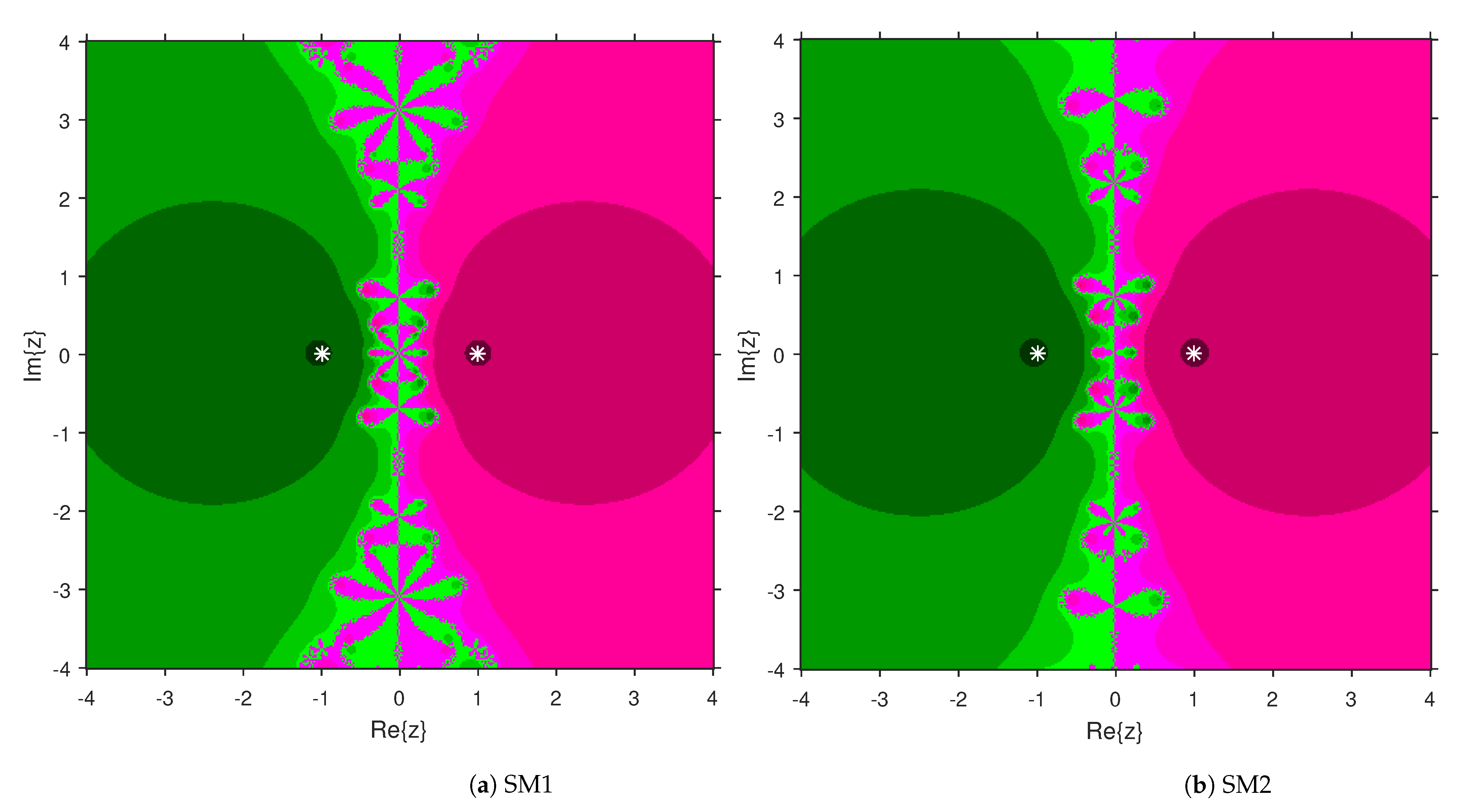
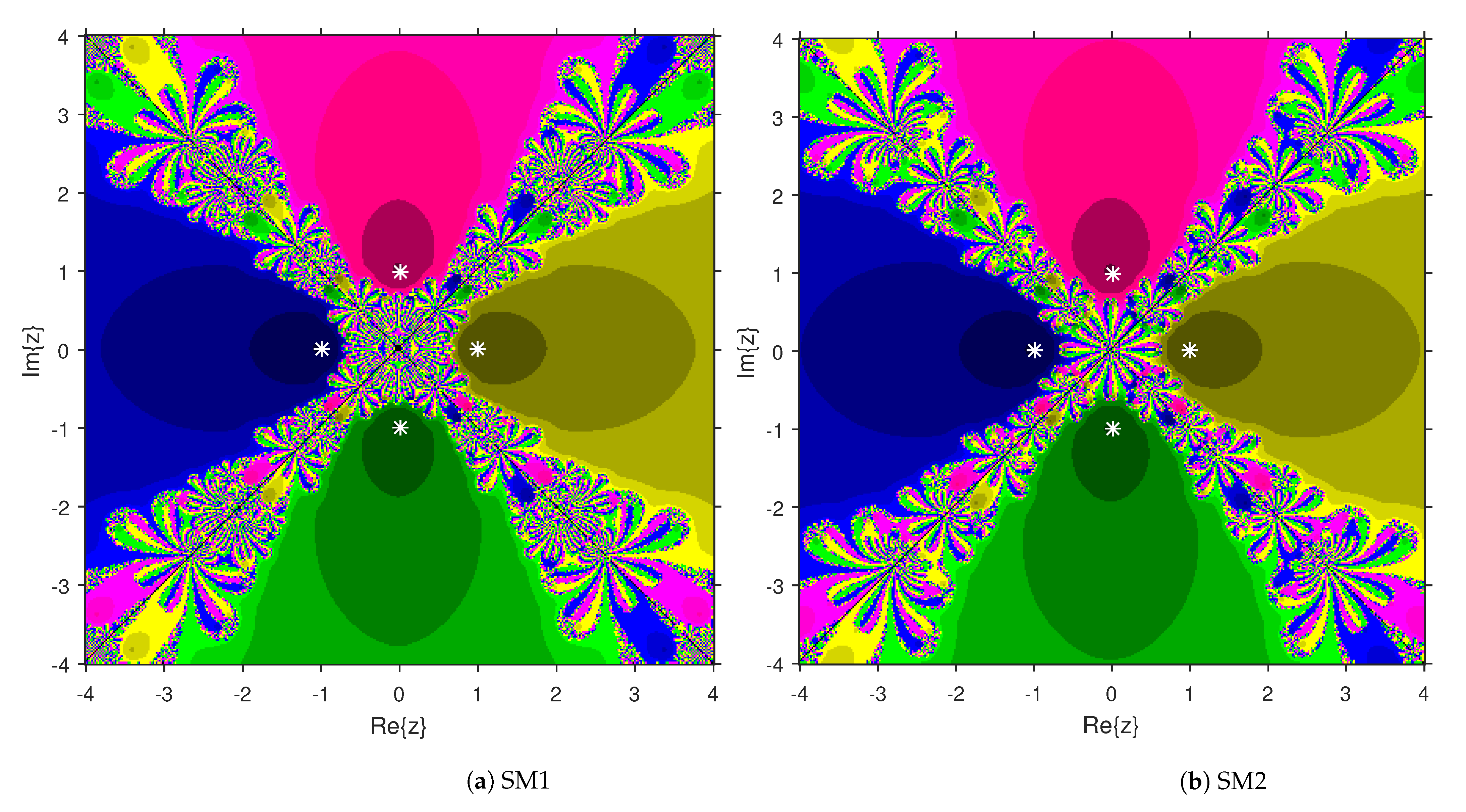
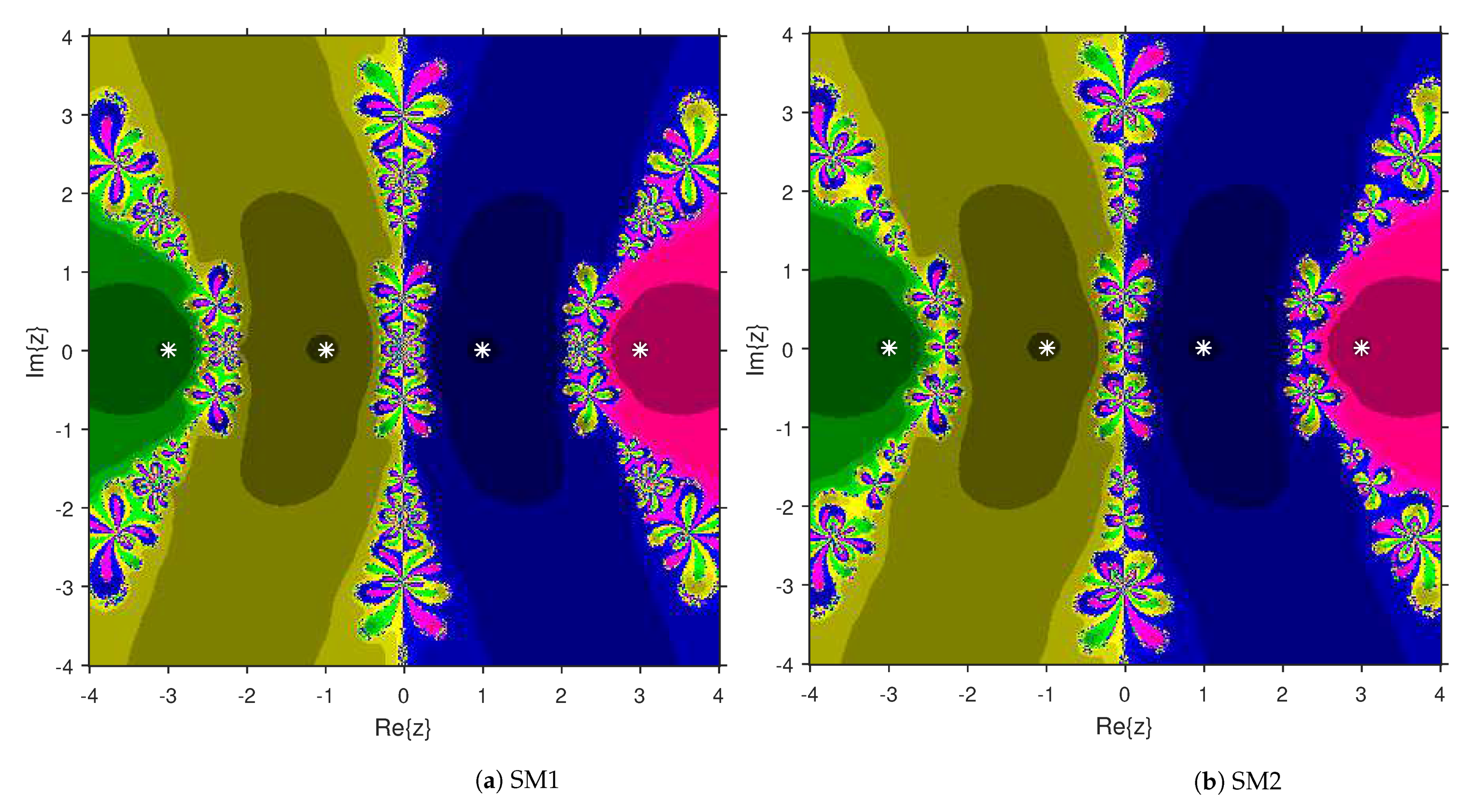
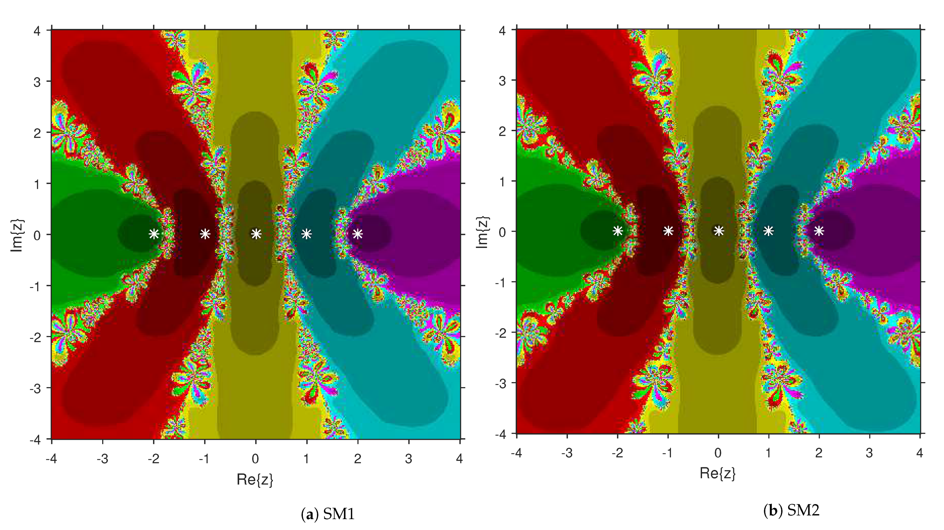
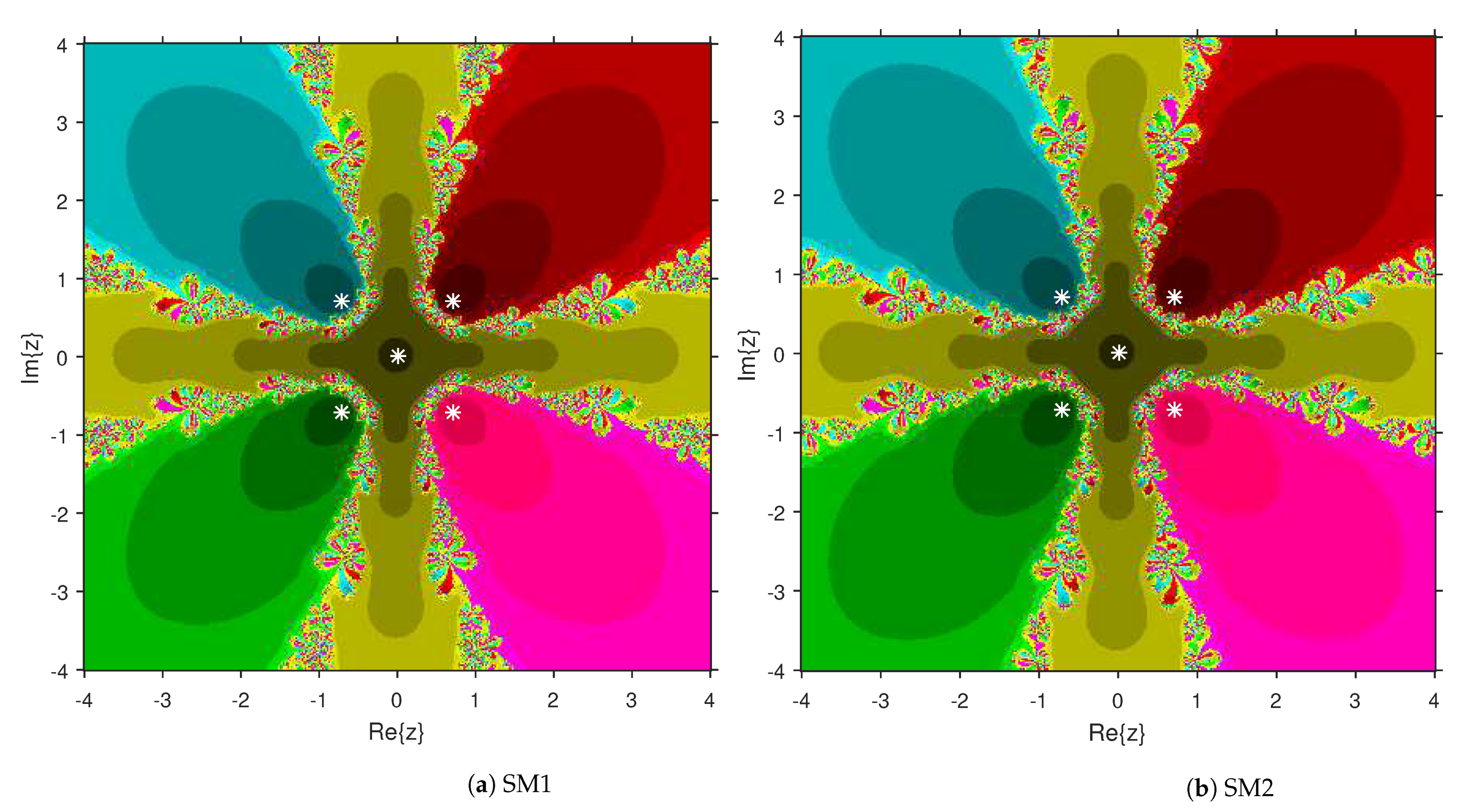
Comparison of the dynamical qualities of SM1 and SM2 are provided in this section by employing the tool attraction basin. Suppose $\mathcal{M}\left(z\right)$ is the notation for a second or higher degree complex polynomial. Then, the set $\{z_0\in \mathbb{C}:z_j\to z_{*}asj\to \infty \}$ represents the attraction basin corresponding to a zero $z_{*}$ of $\mathcal{M}$, where ${\left\{z_j\right\}}_{j=0}^{\infty }$ is formed by an iterative algorithm with a starting choice $z_0\in \mathbb{C}$. Let us select a region $\mathcal{E}=[-4,4]$×$[-4,4]$ on $\mathbb{C}$ with a grid of $400\times 400$ points. To prepare attraction basins, we apply SM1 and SM2 on variety of complex polynomials by selecting every point $z_0\in \mathcal{E}$ as a stater. The point $z_0$ remains in the basin of a zero $z_{*}$ of a considered polynomial if ${\displaystyle \underset{j\to \infty }{lim}{z}_j=z_{*}}$. Then, we display $z_0$ with a fixed color corresponding to $z_{*}$. As per the number of iterations, we employ the light to dark colors to each $z_0$. Black color is the sign of non-convergence zones. The terminating condition of the iteration is $\left|\right|z_j-z_{*}\left|\right|<{10}^{-6}$ with the maximum limit of 300 iterations. We used MATLAB 2019a to design the fractal pictures.

This numerical experiment begins with polynomials ${\mathcal{M}}_1\left(z\right)=z^2-1$ and ${\mathcal{M}}_2\left(z\right)=z^2-z-1$ of degree two. These polynomials are used to compare the attraction basins for SM1 and SM2. The results of comparison are displayed in Figure 1 and Figure 2. In Figure 1, green and pink areas indicate the attraction basins corresponding to the zeros $-1$ and 1, respectively, of ${\mathcal{M}}_1\left(z\right)$. 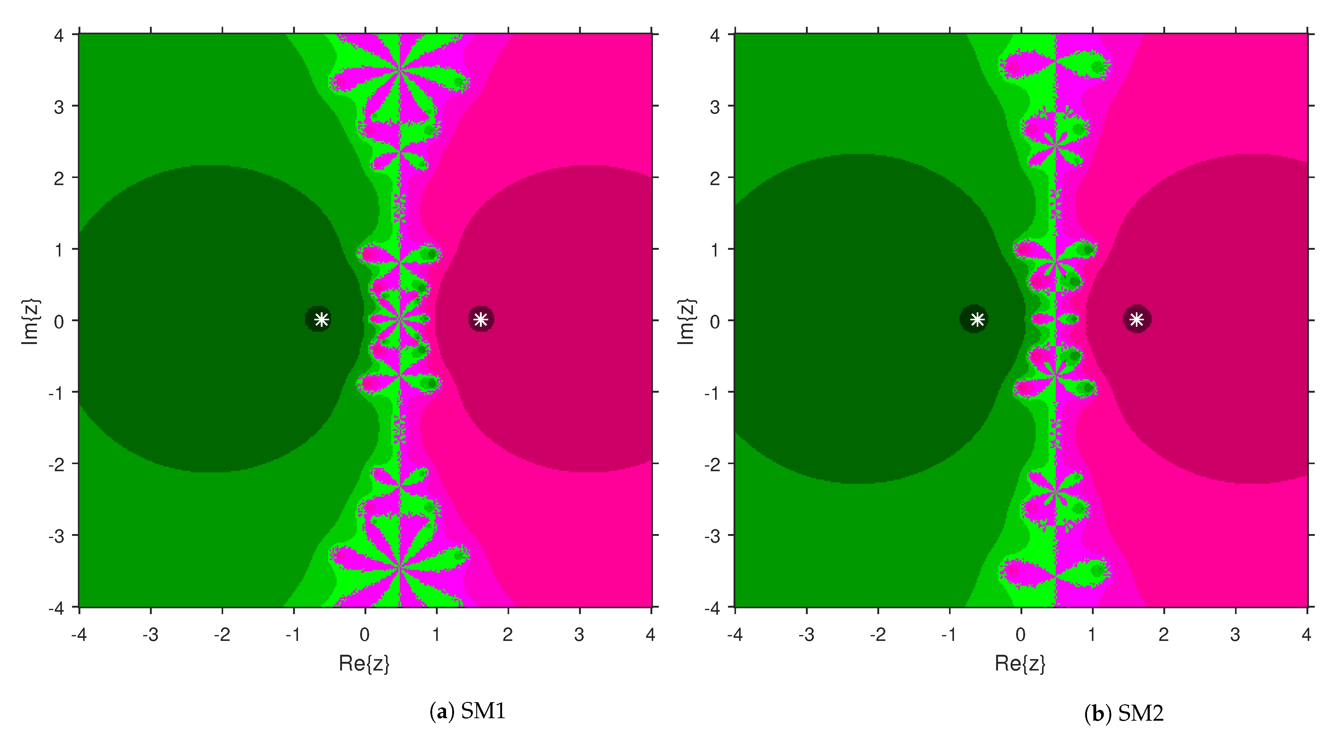The basins of the solutions $\frac{1+\sqrt{5}}{2}$ and $\frac{1-\sqrt{5}}{2}$ of ${\mathcal{M}}_2\left(z\right)=0$ are shown in Figure 2 by applying pink and green colors, respectively. 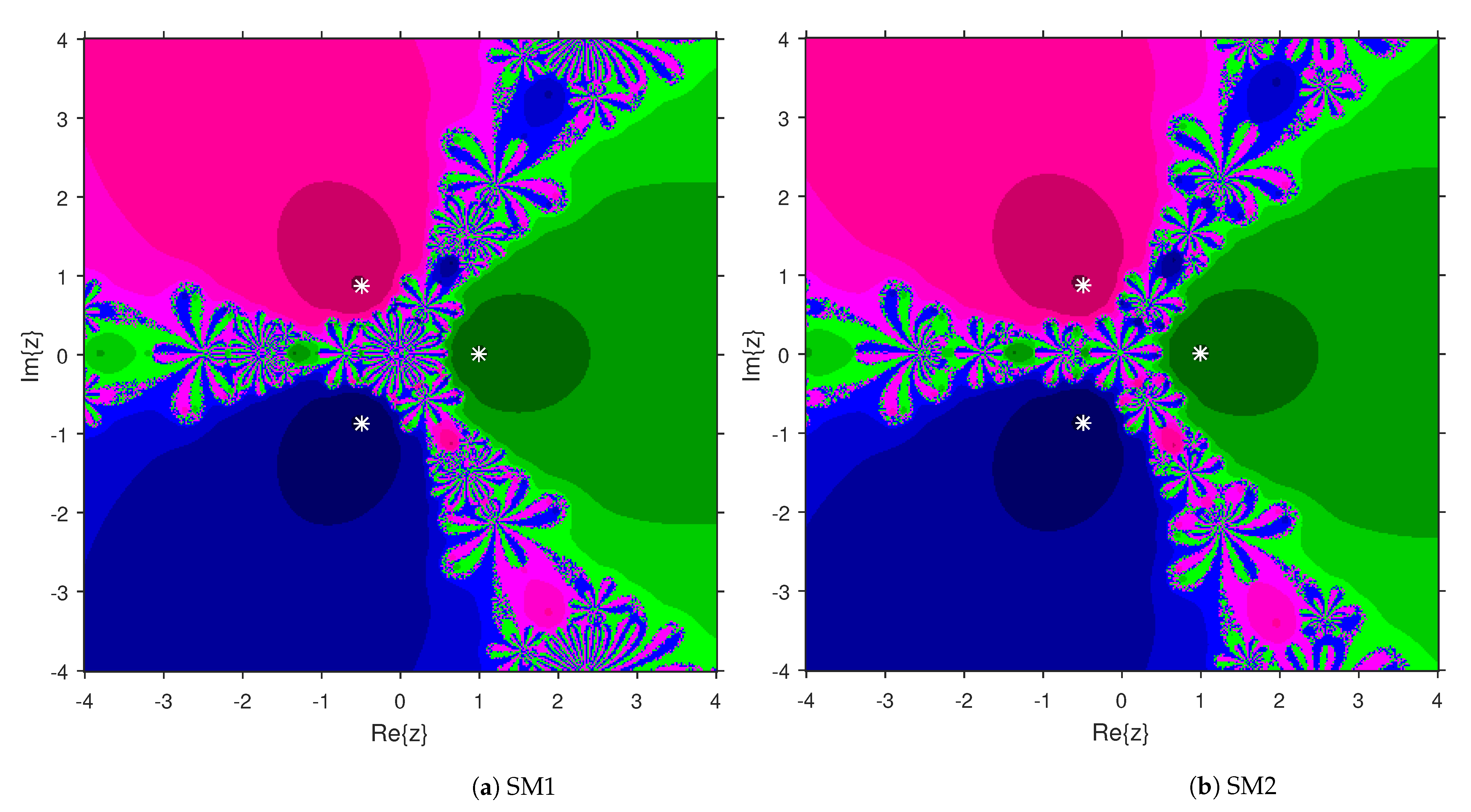Figure 3 and Figure 4 offer the attraction basins for SM1 and SM2 associated to the zeros of ${\mathcal{M}}_3\left(z\right)=z^3-1$ and ${\mathcal{M}}_4\left(z\right)=z^3+(-0.7250+1.6500i)z-0.275-1.65i$. 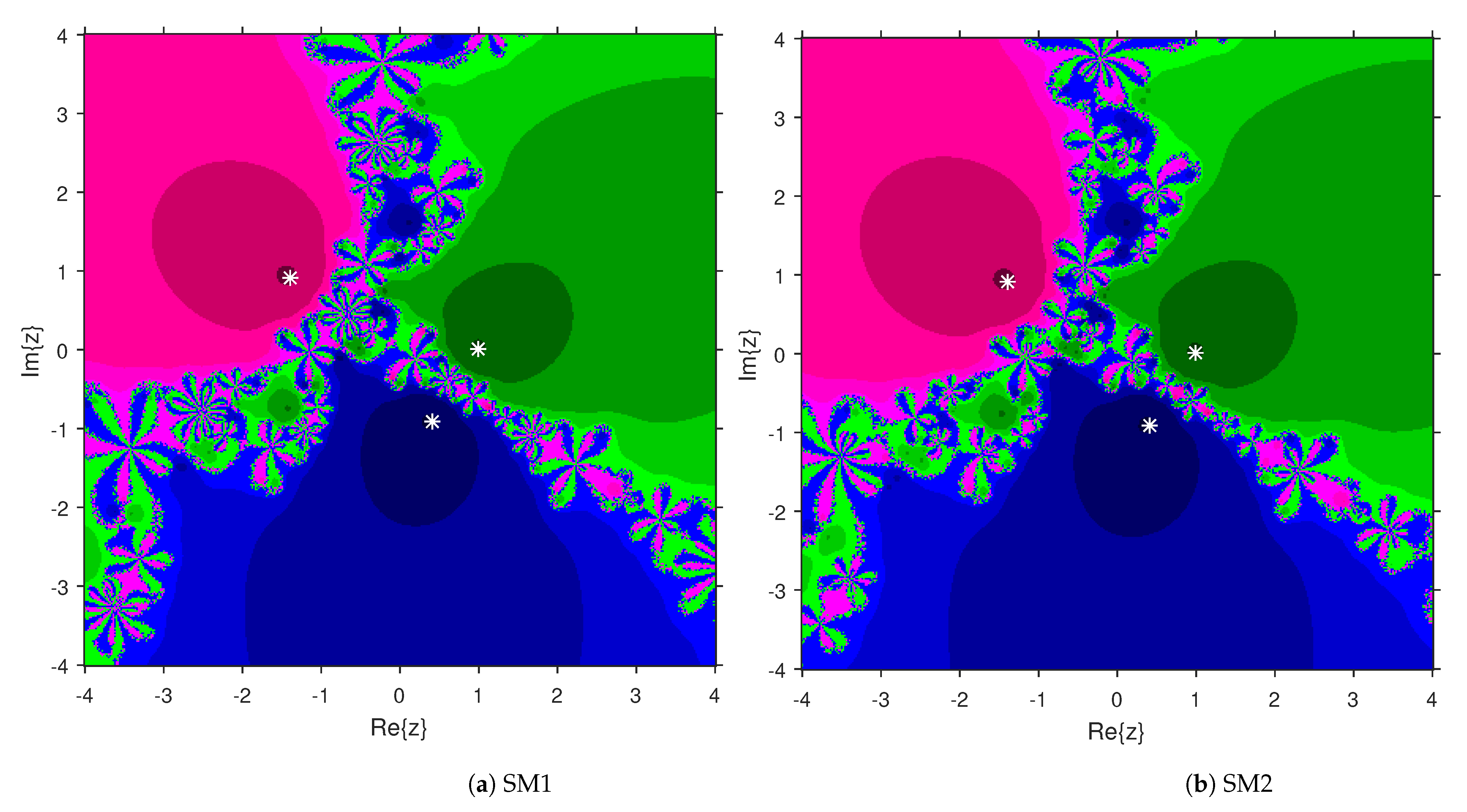In Figure 3, the basins of the solutions $-\frac{1}{2}-0.866025i$, 1 and $-\frac{1}{2}+0.866025i$ of ${\mathcal{M}}_3\left(z\right)=0$ are painted in blue, green and pink, respectively. The basins for SM1 and SM2 associated to the zeros 1, $-1.401440+0.915201i$ and $0.4014403-0.915201i$ of ${\mathcal{M}}_4\left(z\right)$ are given in Figure 4 by means of green, pink and blue regions, respectively. Next, we use polynomials ${\mathcal{M}}_5\left(z\right)=z^4-1$ and ${\mathcal{M}}_6\left(z\right)=z^4-10z^2+9$ of degree four to compare the attraction basins for SM1 and SM2. Figure 5 provides the comparison of basins for these algorithms associated to the solutions 1, $-i$, i and $-1$ of ${\mathcal{M}}_5\left(z\right)=0$, which are denoted in yellow, green, pink and blue regions. The basins for SM1 and SM2 corresponding to the zeros $-1$, 3, $-3$ and 1 of ${\mathcal{M}}_6\left(z\right)$ are demonstrated in Figure 6 using yellow, pink, green and blue colors, respectively. Moreover, we select polynomials ${\mathcal{M}}_7\left(z\right)=z^5-5z^3+4z$ and ${\mathcal{M}}_8\left(z\right)=z^5+z$ of degree five to design and compare the attraction basins for SM1 and SM2. Figure 7 gives the basins of zeros 0, 2, $-1$, $-2$ and 1 of ${\mathcal{M}}_7\left(z\right)$ in yellow, magenta, red, green and cyan colors, respectively. In Figure 8, green, cyan, red, pink and yellow regions illustrate the attraction basins of the solutions $-0.707106-0.707106i$, $-0.707106+0.707106i$, $0.707106+0.707106i$, $0.707106-0.707106i$ and 0, respectively, of ${\mathcal{M}}_8\left(z\right)=0$. 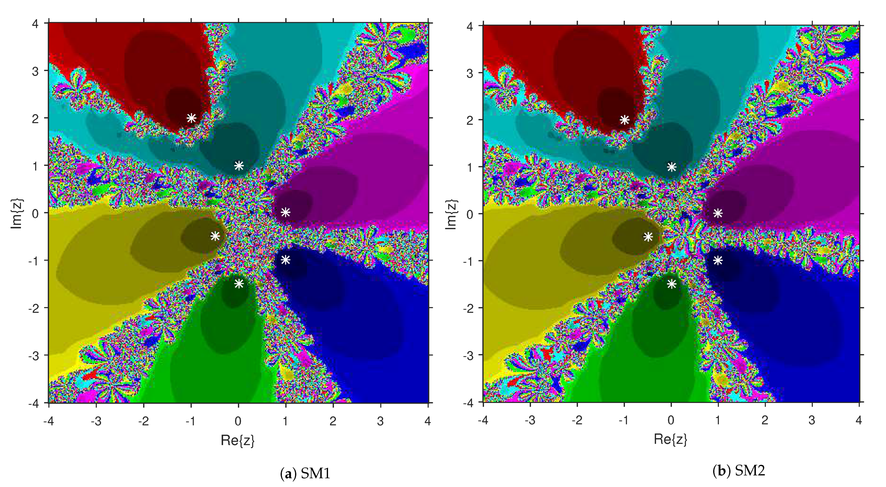Lastly, sixth degree complex polynomials ${\mathcal{M}}_9\left(z\right)=z^6-0.5z^5+\frac{11}{4}(1+i)z^4-\frac{1}{4}(19+3i)z^3+\frac{1}{4}(11+i)z^2-\frac{1}{4}(19+3i)z+\frac{3}{2}-3i$ and ${\mathcal{M}}_{10}\left(z\right)=z^6+z-1$ are considered. In Figure 9, the attraction basins for SM1 and SM2 corresponding to the zeros $1-i$, $-\frac{1}{2}-\frac{i}{2}$, $-\frac{3}{2}i$, 1, i and $-1+2i$ of ${\mathcal{M}}_9\left(z\right)$ are given in blue, yellow, green, magenta, cyan and red colors, respectively. In Figure 10, green, pink, red, yellow, cyan and blue colors are applied to illustrate the basins related to the solutions $-1.134724$, $0.629372-0.735755i$, $0.7780895$, $-0.451055-1.002364i$, $0.629372+0.735755i$ and $-0.451055+1.002364i$ of ${\mathcal{M}}_{10}\left(z\right)=0$, respectively. In these Figure 1, Figure 2, Figure 3, Figure 4, Figure 5, Figure 6, Figure 7, Figure 8, Figure 9 and Figure 10, the roots of the considered polynomials are displayed using white *.

Figure 1. Attraction basins comparison between SM1 and SM2 related to ${\mathcal{M}}_1\left(z\right)$.

Figure 2. Attraction basins comparison between SM1 and SM2 corresponding to ${\mathcal{M}}_2\left(z\right)$.

Figure 3. Attraction basins comparison between SM1 and SM2 related to ${\mathcal{M}}_3\left(z\right)$.

Figure 4. Attraction basins comparison between SM1 and SM2 corresponding to ${\mathcal{M}}_4\left(z\right)$.

Figure 5. Attraction basins comparison between SM1 and SM2 related to ${\mathcal{M}}_5\left(z\right)$.

Figure 6. Attraction basins comparison between SM1 and SM2 corresponding to ${\mathcal{M}}_6\left(z\right)$.

Figure 7. Attraction basins comparison between SM1 and SM2 related to ${\mathcal{M}}_7\left(z\right)$.

Figure 8. Attraction basins comparison between SM1 and SM2 corresponding to ${\mathcal{M}}_8\left(z\right)$.

Figure 9. Attraction basins comparison between SM1 and SM2 related to ${\mathcal{M}}_9\left(z\right)$.

Figure 10. Attraction basins comparison between SM1 and SM2 corresponding to ${\mathcal{M}}_{10}\left(z\right)$.

4. Numerical Examples

We apply the proposed techniques to estimate the convergence radii for SM1 and SM2 when $\alpha =\frac{2}{3}$.

Example 1.

Let us consider ${\mathcal{Y}}_1={\mathcal{Y}}_2=C[0,1]$ and $\mathcal{Z}=\overline{U}(0,1)$. Define $\mathcal{X}$ on $\mathcal{Z}$ by

$$\mathcal{X}\left(v\right)\left(a\right)=v\left(a\right)-5{\int }_0^{1}axv{\left(x\right)}^{3}dx,$$

where $v\left(a\right)\in C[0,1]$. We have $v_{*}=0$. In addition, ${\lambda }_0\left(s\right)=7.5s$, $\lambda \left(s\right)=15s$ and ${\lambda }_1\left(s\right)=2$. The values of ρ and $\overline{\rho }$ are produced by the application of proposed theorems and summarized in Table 1.

Table 1. Comparison of convergence radii for Example 1.

SM1	SM2
${\rho }_1=0.022222$	$\overline{{\rho }_1}=0.022222$
${\rho }_2=0.023424$	$\overline{{\rho }_2}=0.021456$
${\rho }_3=0.006858$	$\overline{{\rho }_3}=0.006703$
$\rho =0.006858$	$\overline{\rho }=0.006703$

Example 2.

Let ${\mathcal{Y}}_1={\mathcal{Y}}_2={\mathbb{R}}^3$ and $\mathcal{Z}=\overline{U}(0,1)$. Consider $\mathcal{X}$ on $\mathcal{Z}$ for $v={(v_1,v_2,v_3)}^t$ as

$$\mathcal{X}\left(v\right)={(e^{v_1}-1,\frac{e-1}{2}{v}_2^2+v_2,v_3)}^t$$

We have $v_{*}={(0,0,0)}^t$. In addition, ${\lambda }_0\left(s\right)=(e-1)s$, $\lambda \left(s\right)=e^{\frac{1}{e-1}}s$ and ${\lambda }_1\left(s\right)=2$. Using the newly proposed theorems the values of ρ and $\overline{\rho }$ are calculated and displayed in Table 2.

Table 2. Comparison of convergence radii for Example 2.

SM1	SM2
${\rho }_1=0.127564$	$\overline{{\rho }_1}=0.127564$
${\rho }_2=0.113416$	$\overline{{\rho }_2}=0.102805$
${\rho }_3=0.033574$	$\overline{{\rho }_3}=0.032642$
$\rho =0.033574$	$\overline{\rho }=0.032642$

Example 3.

Finally, the motivational problem described in the first section is addressed with $v_{*}=1$, ${\lambda }_0\left(s\right)=\lambda \left(s\right)=96.662907s$ and ${\lambda }_1\left(s\right)=2$. We apply the suggested theorems to compute ρ and $\overline{\rho }$. These values are shown in Table 3.

Table 3. Comparison of convergence radii for Example 3.

SM1	SM2
${\rho }_1=0.002299$	$\overline{{\rho }_1}=0.002299$
${\rho }_2=0.002026$	$\overline{{\rho }_2}=0.001835$
${\rho }_3=0.000600$	$\overline{{\rho }_3}=0.000583$
$\rho =0.000600$	$\overline{\rho }=0.000583$

It is worth noticing that if we stop at the first iterate in both algorithms (i.e., restrict ourselves to the first substep of Jarratt’s algorithm), then the radius is largest (see ${\rho }_1$ and $\overline{{\rho }_1}$). Moreover, if we increase the convergence order to four (i.e., consider only the first two substeps of the algorithms), then the radii get smaller (see ${\rho }_2$ and $\overline{{\rho }_2}$). Furthermore, if we increase the order to six (i.e., use all the substeps of these algorithms), then, we obtain the smallest radii (see $\rho$ and $\overline{\rho }$). This is expected when the order increases. Concerning the corresponding error estimates $\left|\right|v_n-v_{*}\left|\right|$ we see clearly that fewer iterates are needed to reach $v_{*}$ as order increases. We solved Example 3 with $v_0=0.9993$ using these algorithms and the results are presented in Table 4 and Table 5. In addition, we executed four iterations of these schemes ten times in MATLAB 2019a. Then, we obtained the average elapsed time and average CPU time (in seconds) for SM1 and SM2 and these values are presented in Table 6.

Table 4. $\left|\right|v_n-v_{*}\left|\right|$ for algorithm SM1.

n	1 Substep	2 Substeps	3 Substeps (SM1)
1	$2.32\times {10}^{-4}$	$1.29\times {10}^{-11}$	$3.65\times {10}^{-14}$
2	$7.73\times {10}^{-5}$	$1.50\times {10}^{-42}$	$1.38\times {10}^{-65}$
3	$2.58\times {10}^{-5}$	$2.74\times {10}^{-166}$	$1.06\times {10}^{-322}$
4	$8.59\times {10}^{-6}$	$3.00\times {10}^{-661}$	$2.87\times {10}^{-1608}$

Table 5. $\left|\right|v_n-v_{*}\left|\right|$ for algorithm SM2.

n	1 Substep	2 Substeps	3 Substeps (SM2)
1	$2.32\times {10}^{-4}$	$7.12\times {10}^{-12}$	$2.01\times {10}^{-14}$
2	$7.73\times {10}^{-5}$	$7.59\times {10}^{-44}$	$3.83\times {10}^{-67}$
3	$2.58\times {10}^{-5}$	$9.81\times {10}^{-172}$	$9.67\times {10}^{-331}$
4	$8.59\times {10}^{-6}$	$2.73\times {10}^{-683}$	$9.96\times {10}^{-1649}$

Table 6. Elapsed time and CPU time comparison between SM1 and SM2.

Algorithm	Elapsed Time	CPU Time
$SM1$	$3.2925$	$3.4875$
$SM2$	$3.4524$	$3.6187$

5. Conclusions

Major problems appear when studying high convergence order algorithms for solving equations. One of them is that the order is shown assuming the existence of higher order derivatives that do not appear on the algorithms. In particular in the case of SM1 ans SM2 derivatives up to the order seven have been utilized. Hence (see also our example in the introduction) these derivative restrict the utilization of these algorithms. We also do not know how many iterates needed to arrive at a prearranged accuracy. Moreover, no uniqueness of the solution is known about a certain ball. This is not only the case for the algorithms we studied but all the high convergence algorithms whose convergence order is shown using Taylor series. That is why we addressed all these concerns in the more general situation of a Banach space, under generalized continuity conditions and using only the derivative appearing on these algorithms. Our technique can be applied to extend the utilization of other algorithms since it is so general. We also present the convergence ball and dynamical comparison between these schemes.