Comparative Analysis of Recurrent Neural Networks in Stock Price Prediction for Different Frequency Domains

Abstract

Investors in the stock market have always been in search of novel and unique techniques so that they can successfully predict stock price movement and make a big profit. However, investors continue to look for improved and new techniques to beat the market instead of old and traditional ones. Therefore, researchers are continuously working to build novel techniques to supply the demand of investors. Different types of recurrent neural networks (RNN) are used in time series analyses, especially in stock price prediction. However, since not all stocks’ prices follow the same trend, a single model cannot be used to predict the movement of all types of stock’s price. Therefore, in this research we conducted a comparative analysis of three commonly used RNNs—simple RNN, Long Short Term Memory (LSTM), and Gated Recurrent Unit (GRU)—and analyzed their efficiency for stocks having different stock trends and various price ranges and for different time frequencies. We considered three companies’ datasets from 30 June 2000 to 21 July 2020. The stocks follow different trends of price movements, with price ranges of $30, $50, and $290 during this period. We also analyzed the performance for one-day, three-day, and five-day time intervals. We compared the performance of RNN, LSTM, and GRU in terms of $R^2$ value, MAE, MAPE, and RMSE metrics. The results show that simple RNN is outperformed by LSTM and GRU because RNN is susceptible to vanishing gradient problems, while the other two models are not. Moreover, GRU produces lesser errors comparing to LSTM. It is also evident from the results that as the time intervals get smaller, the models produce lower errors and higher reliability.

1. Introduction

A stock market is a place where companies issue their stocks to enlarge their business and investors can buy/sell the stocks to each other at specific prices. Investors around the world can buy a company’s stock and enjoy yearly dividends for their shares. They can also sell their stocks at any time and can make a profit by selling at a price higher than their buying. The stock market is becoming a crucial investment venue, and the size of the market is growing every day. As of January 2021, the top 10 stock exchanges have $81.68 trillion worth of total capitalization [1]. Although stock market investment seems lucrative, predicting stock movements in competitive financial markets is a challenge, even for experienced traders and stock experts. However, stock price forecasting theory is often controversial: within a fraction of a second, the price of a stock can fluctuate so drastically that some individuals make huge sums of money, leaving the rest of the shareholders in financial ruin. Even after that, many experts and economists have been continuously trying to make stock predictions using a variety of methods for the past few decades. However, manually predicting stock price trends from stock data is a tedious task. However, now, with the advent of artificial intelligence, the automated method of predicting the stock market through big data and enhanced computing capabilities has become possible.

The main objective of this research is to predict the stock price using Recurrent Neural Networks (RNN) for three types of stocks: stocks for which price fluctuates significantly, stocks for which the price fluctuates moderately, and stocks for which the price fluctuates slightly. We did our research for three frequency domains: one-day, three-day, and five-day intervals. The motivation for using RNNs compared to other machine learning and statistical approaches is due to their effective prediction capability in time series analysis [2,3,4] and their efficient representation-learning capabilities; raw input transformation can be useful while learning complex functions [5]. The multiple levels of RNN can be utilized for multiple levels of features, which can represent abstract features derived from previous levels, and thus, the level of abstraction is increased. Compared to typical networks with one hidden layer, RNN can achieve a higher level of feature extraction by adding extra hidden layers [6,7]. The adaptability of RNNs in a complex financial market acts as the primary motivation to analyze the performance of RNNs with stock market data.

The outline of this article is as follows: Section 2 discusses related works in stock price prediction and briefly introduces RNN, LSTM, and GRU models; Section 3 explains the proposed methodology, Section 4 discusses the outcomes of the research, and Section 5 concludes with the overall findings and discusses future research directions.

2. Background

2.1. Related Works

This research lies in the wide research area of Efficient Market Hypothesis proposed by Eugena F. Fama [8,9]. Fama said that we can just test whether data are appropriately reflected in costs with regards to an evaluating model. A 1970 survey isolates work on market productivity into three categories: (i) weak-form tests (how well do past returns foresee future returns?), (ii) semi strong-form tests (how rapidly do security costs reflect public data declarations?), and (iii) strong-form tests (do any financial backers have private data that is not completely reflected in market costs?). This work can also be categorized as big data research, as we have considered stock data of the timeframe 2000–2020 [10].

There are several methods in computer science as well as in economics to predict the future behavior of the market, which includes the direction of stock trend (up or down, i.e., bull market or bear market, respectively), costing of stock on intraday or interday, related risk and return, etc. A finite sequence or a collection of data points gathered at explicit periods indicates the time-series data of the stock market. It refers to information about the stock during the specific trading cycle of a stock exchange; such recorded information in its crude structure incorporates the starting and ending prices, the most noteworthy and least costs achieved, and the complete number of exchanged stocks, i.e., volume, for the specified period of trading. Several machine learning techniques have been applied to predict stock price movement [11,12,13]. In order to obtain appropriate predictions, this materialistic stock data have been merged with computational intellectual-based procedures [14,15,16] and different econometrics-based factual strategies [17,18,19]. The numerical techniques are probably going to be subject to the underlying presumptions; on the contrary, the AI approaches experience controlled interoperability, performing based on manually selected features, and over-fitting issues; this supports a mix of neural network (NN)-based deep learning strategies to upgrade the predictions of the stock market [20,21,22]. By using such NNs, the main characteristics of the supremely unstructured data can be extracted, which is useful in studying the hidden patterns of the movement of the stock price [23]. The stock market is affected by a number of events, and their impact is difficult to identify [24]; economic markets can be assessed by studying and analyzing such phenomena. The study provides evidence on the impact of political influence [25], data protection events [26], specific news and/or announcements [27], national policies [28], and other factors. The investigation through this angle is critical; likewise, the potential security perspectives on domains related to the monetary business sectors are urgent to keep up the integrity of the gathered data as well as their analysis [29,30]. In addition, it is important to understand the potential effects of several domains on financial market volatility.

In this research, we want to justify the use of recurrent neural networks using three popular versions of RNN: Simple RNN, Long Short Term Memory (LSTM), and Gated Recurrent Unit (GRU). Although many approaches are used to predict stock price, a model loses its viability when everyone starts using the same method. Therefore, investors are always in search of new approaches to outperform previous techniques. We do not only focus on the viability of neural networks in stock price forecasting, but also aim to show how different versions of RNN behave with different types of stocks. To serve that purpose, we considered Honda Motor Company’s dataset as slightly fluctuating data whose stock price are in between USD 15 to USD 45 in the duration 2000–2020. We also considered Oracle Corporation as the moderately fluctuating data (price range USD 10 to USD 60), and Intuit Incorporation as the highly fluctuating data which had the lowest price of USD 20 and the highest price of USD 310. These three datasets were considered as proofs of concept, and the models can be applied to any other datasets as well. All datasets are collected from Yahoo Finance.

2.2. Overview of Recurrent Neural Networks

A Recurrent Neural Network (RNN) is an advanced form of neural networks that has internal memory that makes RNN capable of processing long sequences [31]. This makes RNN very suitable for stock price prediction, which involves long historical data. The following three subsections briefly discuss simple RNN, LSTM, and GRU models.

2.2.1. Simple RNN Model

RNN can provide considerably good prediction for the temporal stock data. The hidden states of RNN are given by Equations (1) and (2) [32].

$$S_t=tanh(W{x}_t+U{S}_{t-1}+b)$$

(1)

$$o_t=c+V{S}_t$$

(2)

where $x_t$ is the input vector at time t; b and c are bias values; W, U, and V denote input-to-hidden, hidden-to-hidden, and hidden-to-output weight matrices, respectively. While working with time-series data (like the stock market), an attention mechanism can be utilized that can divide the given data into parts so that decoder can utilize specific parts while generating new values. Figure 1 shows the generalized RNN architecture [33].

2.2.2. LSTM Model

LSTM network is a modified version of recurrent neural networks, which makes it easier to remember past data in memory. The vanishing gradient problem of RNN is resolved here. LSTM is well-suited to classification process and time series prediction given time lags of unknown duration. It trains the model using back-propagation. LSTM architecture consists of five main parts (Figure 2) [34,35]:

• Cell state ($c_t$)—1D vector of fixed shape with random value initialization. It contains the information that was present in the memory after the previous time step.
• Forget gate ($f_t$)—changes the cell state, intending to eliminate non-important values from previous time steps. This helps the LSTM network to forget the irrelevant information that does not have any impact on the future price prediction.
• Input gate ($i_t$)—changes the cell state with the aim of adding new information about the current time step. It adds new information that may affect the stock price movement.
• Output gate ($o_t$)—decides what the next hidden state should be. The new cell state and the new hidden is then carried over to the next time step. Returns the final relevant information, which will be used for stock price prediction.
• Hidden state ($h_t$)—it is calculated by multiplying output gate vector by cell state vector.

The values of these vectors are calculated by the Equations (3)–(7).

$$i_t=\sigma (W^{\left(i\right)}{x}_t+U^{\left(i\right)}{h}_{t-1}+b^{\left(i\right)})$$

(3)

$$f_t=\sigma (W^{\left(f\right)}{x}_t+U^{\left(f\right)}{h}_{t-1}+b^{\left(f\right)})$$

(4)

$$o_t=\sigma (W^{\left(o\right)}{x}_t+U^{\left(o\right)}{h}_{t-1}+b^{\left(o\right)})$$

(5)

$$c_t=i_t\odot u_t+f_t\odot c_{t-1}$$

(6)

$$h_t=o_t\odot tanh\left(c_t\right)$$

(7)

where $x_t$ is input vector, $c_{t-1}$ is previous cell state, $h_{t-1}$ is previous hidden state, W and U are input-to-hidden and hidden-to-hidden weight matrices, $\sigma$ is the logistic sigmoid function, and ⊙ denotes the element-wise multiplication.

2.2.3. GRU Model

Like LSTM, GRU is another improved version of the standard RNN. To solve the vanishing gradient problem of a standard RNN, GRU uses an update gate and reset gate. These are two vectors that decide what information should be passed to the output. The special thing about them is that they can be trained to keep information from long ago without washing it through time or to remove information that is irrelevant to the prediction. To explain the mathematics behind that process, we will examine a single unit of GRU given in Figure 3 [36,37].

The update gate helps the model to determine how much of the past information (from previous time steps) needs to be passed along to the future. This is very powerful because the model can decide to copy all the information from the past and eliminate the risk of the vanishing gradient problem. It is calculated by Equation (8).

$$z_t=\sigma (W^{\left(z\right)}{x}_t+U^{\left(z\right)}{h}_{t-1}+b^{\left(z\right)})$$

(8)

A reset gate is used to decide how much of the past information to forget and is calculated by Equation (9).

$$r_t=\sigma (W^{\left(r\right)}{x}_t+U^{\left(r\right)}{h}_{t-1}+b^{\left(r\right)})$$

(9)

The final output of the cell is calculated by the Equation (10).

$$r_t=z_t\odot h_{t-1}+(1-z_t)\odot \widetilde{h_t})$$

(10)

where candidate activation vector, $\widetilde{h_t}=tanh(W{x}_t+r_t\odot U{h}_{t-1}+b^{\left(h\right)})$.

3. Proposed Methodology

In this research, we have analyzed the effectiveness of Recurrent Neural Networks (Simple RNN, LSTM, and GRU) while predicting different types of stocks’ price movements. Specifically, we considered three types of datasets—highly fluctuated, moderately fluctuated, and slightly fluctuated—and the prediction was done for three different time intervals: one day, three days, and five days. Figure 4 shows the system architecture of our proposed model.

3.1. Data Collection

As slightly fluctuating data, we considered Honda Motor Company (HMC), and the dataset was collected from Yahoo Finance [38]. We considered Orcale Corporation (ORCL)’s data as a moderately fluctuating dataset, and Intuit Inc. (INTU)’s data as a highly fluctuated dataset, which was also collected from Yahoo Finance [39,40]. For all of these datasets, we collected the data for 20 years (from 30 June 2000 to 21 July 2020) and have 5044 instances in each dataset. Each dataset contains seven attributes: date, open price, high price, low price, close price, adjusted close price, and traded volume.

3.2. Data Preprocessing

There were few null values in the collected datasets. As null value can disrupt the actual pattern of the price movement, it can handle the null values efficiently. A widely employed method to replace the null value is to use the mean of the previous 30 days’ price. We used this method to solve this issue. Moreover, we collected data in the format of one-day time intervasl. Therefore, for our one-day proposed model, there was no preprocessing needed. However, for three-day and five-day models, we had to convert one-day time-interval data into three-day and five-day time-interval datasets. For this purpose, we made the following adjustments:

• Date: Date of the first day of the 3 days and 5 days timeframe;
• Open Price: Opening price of the first day of the 3 days and 5 days timeframes;
• High Price: Highest price in the entire 3 days and 5 days timeframe;
• Low Price: Lowest price in the entire 3 days and 5 days timeframes;
• Close Price: Closing price of the last day of the 3 days and 5 days timeframes;
• Traded Volume: Total traded volume in the entire 3 days and 5 days timeframes.

3.3. Model Design

To reiterate, we have predicted the stock price movements for three different stocks (HMC, ORCL, and INTU) of various fluctuation for three different frequencies (1 day, 3 days, and 5 days) using three neural networks models (Simple RNN, LSTM, and GRU). Therefore, we built a total of 27 models for our analysis. Each model was trained on 80% of the total data and was tested on 20% data. We used the corresponding neural network (RNN, LSTM, or GRU) as the first hidden layer, followed by a 20% dropout layer. Adam optimizer was used as the model optimizer, and MSE was used as loss function. After analyzing the effect of various neuron combinations in the hidden layers, we propose that the following neuron combinations work best on different trends in the three frequency domains.

Table 1. Model Architecture for Slightly Fluctuating Data (HMC).

Timeframe	Model	First Layer	Second Layer
one-day	RNN	64	64
	LSTM	256	256
	GRU	512	1024
three-day	RNN	128	128
	LSTM	256	256
	GRU	512	256
five-day	RNN	128	32
	LSTM	256	128
	GRU	512	1024

,

Table 2. Model Architecture for Moderately Fluctuating Data (ORCL).

Timeframe	Model	First Layer	Second Layer
one-day	RNN	256	64
	LSTM	256	128
	GRU	512	512
three-day	RNN	64	128
	LSTM	256	256
	GRU	256	512
five-day	RNN	256	64
	LSTM	256	256
	GRU	256	128

and

Table 3. Model Architecture for Highly Fluctuating Data (INTU).

Timeframe	Model	First Layer	Second Layer
one-day	RNN	64	256
	LSTM	256	128
	GRU	512	1024
three-day	RNN	128	128
	LSTM	1024	512
	GRU	1024	512
five-day	RNN	256	128
	LSTM	256	512
	GRU	1024	512

show the number of neurons used in each model.

3.4. Model Validation

To validate our model, we used four performance metrics: Mean Absolute Error (MAE), Mean Absolute Percentage Error (MAPE), Root Mean Squared Error (RMSE), and R squared value ($R^2$). MAE and MAPE only consider the amount of the error, not the sign. Therefore, it eliminates the possibility of positive and negative errors canceling each other otu. RMSE takes the square of the error before averaging it, and therefore, it gives more weight to the large error. It is therefore more useful when the high error is undesirable like stock price prediction. Finally, the $R^2$ value indicates the risk associated with a model while predicting a financial asset’s price.

Mean Absolute Error (MAE) measures the absolute average error between the real data and predicted data and is calculated using the Equation (11).

$$MAE=\frac{1}{N}\sum _{j=1}^N|y_j-y_j^{{}^{\prime }}|$$

(11)

where $y_j$ = actual value, $y_j^{{}^{\prime }}$ = predicted value, N = total number test cases, and j = value ranging from 1 to N.

Mean Absolute Percentage Error (MAPE) is the mean of absolute percentage error where the error is defined as the absolute difference between actual and predicted value [41]. MAPE is easy to understand as the error is represented in terms of percentage. It is calculated using Equation (12).

$$MAPE=\frac{1}{N}\sum _{t=1}^N\left|\frac{A_t-P_t}{A_t}\right|$$

(12)

where $A_t$ = actual value, $P_t$ = predicted value, N = total number of test cases, and t = value ranging from 1 to N.

Root Mean Squared Error (RMSE) is the rooted value of the squared average distance between the real data and the predicted data and is calculated using Equation (13).

$$RMSE=\sqrt{\frac{1}{N}\sum _{i=1}^N{(A_t-P_t)}^2}$$

(13)

where $A_t$ = actual value, $P_t$ = predicted value, N = total number of test cases.

R Squared Value or the coefficient of determination, is an indicator of goodness of fit of a model. It indicates how close the regression line (i.e., the predicted value curve) is to the actual data values. The R squared value lies between 0 and 1, where 0 indicates that the model cannot capture the correlation among the input and output data, while 1 indicates that the model is perfectly fitted by the dataset. In the financial market, the $R^2$ value is widely used to determine the risk-adjusted return of a financial asset [3]. A higher $R^2$ value indicates lower risk associated with the model and vice versa.

4. Results and Discussions

In this section, we discuss the performance of RNN, LSTM, and GRU on the three datasets for the three different time-intervals. If anyone wants to replicate the results of this research, the authors are willing to share the codes and results. Full codes and results can be downloaded from GitHub (GitHub link: https://github.com/ehfahad/Comparative-Analysis-of-RNNs-in-Stock-Price-Prediction (accessed on 10 July 2021).

4.1. Performance Evaluation of HMC

Figure 5, Figure 6 and Figure 7 show the actual value vs. predicted value curves for one-day time-interval of HMC using RNN, LSTM, and GRU, respectively. All of the models predict very well; however, GRU performs slightly better than the other two models. The results are summarized in

Table 4. Performance comparison of HMC one-day interval.

Model	${\mathit{R}}^2$	MAE	MAPE	RMSE
RNN	0.98321	0.28826	1.03648	0.40842
LSTM	0.98346	0.29185	1.04387	0.40531
GRU	0.98389	0.28329	1.01502	0.40010

.

Actual value vs. predicted value curves for a three-day time-interval of HMC are shown in Figure 8, Figure 9 and Figure 10 where GRU performs better than RNN and LSTM. However, all of them produced slightly larger errors than one-day time-interval, as shown in

Table 5. Performance comparison of HMC three-day interval.

Model	${\mathit{R}}^2$	MAE	MAPE	RMSE
RNN	0.96305	0.43949	1.58962	0.61541
LSTM	0.96204	0.44340	1.58702	0.62375
GRU	0.96413	0.42743	1.54541	0.60643

.

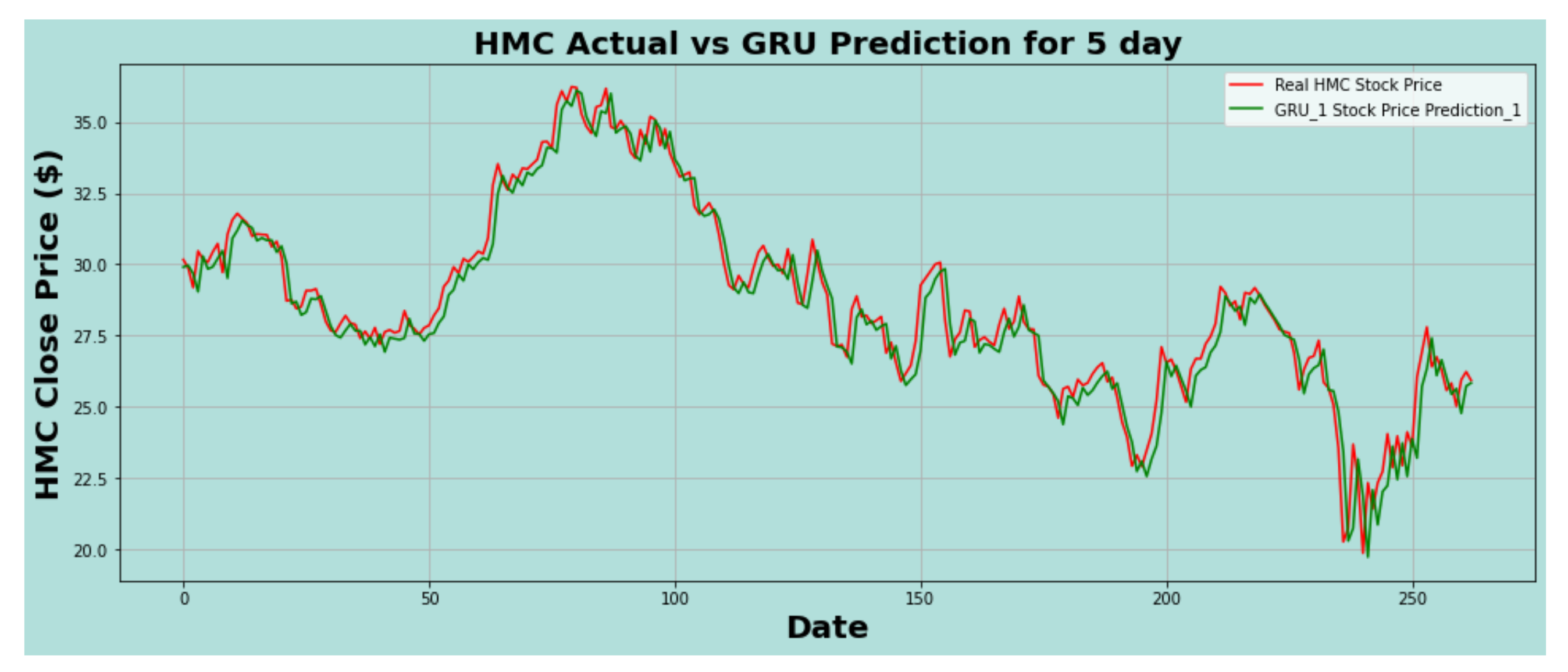
Figure 11, Figure 12 and Figure 13 show the actual vs. predicted curves for five-day time intervals of HMC. GRU outperformed the other two models in this timeframe as well. The results are summarized in

Table 6. Performance comparison of HMC five-day interval.

Model	${\mathit{R}}^2$	MAE	MAPE	RMSE
RNN	0.94284	0.57858	2.10638	0.78400
LSTM	0.94093	0.58079	2.10279	0.79704
GRU	0.96032	0.56959	2.10013	0.78115

.

4.2. Performance Evaluation of ORCL

In case of ORCL dataset, LSTM performs better than RNN and GRU models. The actual vs. predicted value curves of a one-day interval are shown by Figure 14, Figure 15 and Figure 16, of a three-day interval are shown by Figure 17, Figure 18 and Figure 19, and of a five-day interval are shown by Figure 20, Figure 21 and Figure 22.

Table 7. Performance comparison of ORCL one-day interval.

Model	${\mathit{R}}^2$	MAE	MAPE	RMSE
RNN	0.96749	0.64351	1.29133	0.91327
LSTM	0.97345	0.53824	1.10547	0.82530
GRU	0.97295	0.55344	1.18299	0.83296

,

Table 8. Performance comparison of ORCL three-day interval.

Model	${\mathit{R}}^2$	MAE	MAPE	RMSE
RNN	0.95136	0.73144	1.49556	1.06560
LSTM	0.95364	0.70202	1.41944	1.04041
GRU	0.94486	0.83837	1.68504	1.13464

and

Table 9. Performance comparison of ORCL five-day interval.

Model	${\mathit{R}}^2$	MAE	MAPE	RMSE
RNN	0.90040	0.98882	1.98959	1.48361
LSTM	0.90153	0.98621	1.97875	1.39695
GRU	0.90001	0.99962	2.01920	1.40772

summarize the performance of one-day, three-day, and five-day intervals, respectively.

4.3. Performance Evaluation of INTU

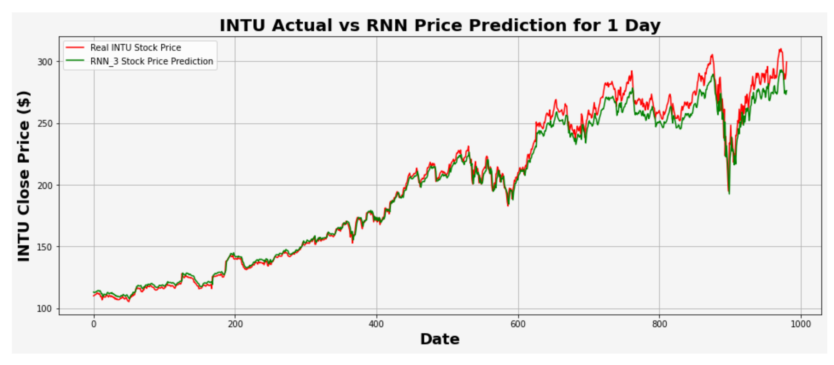
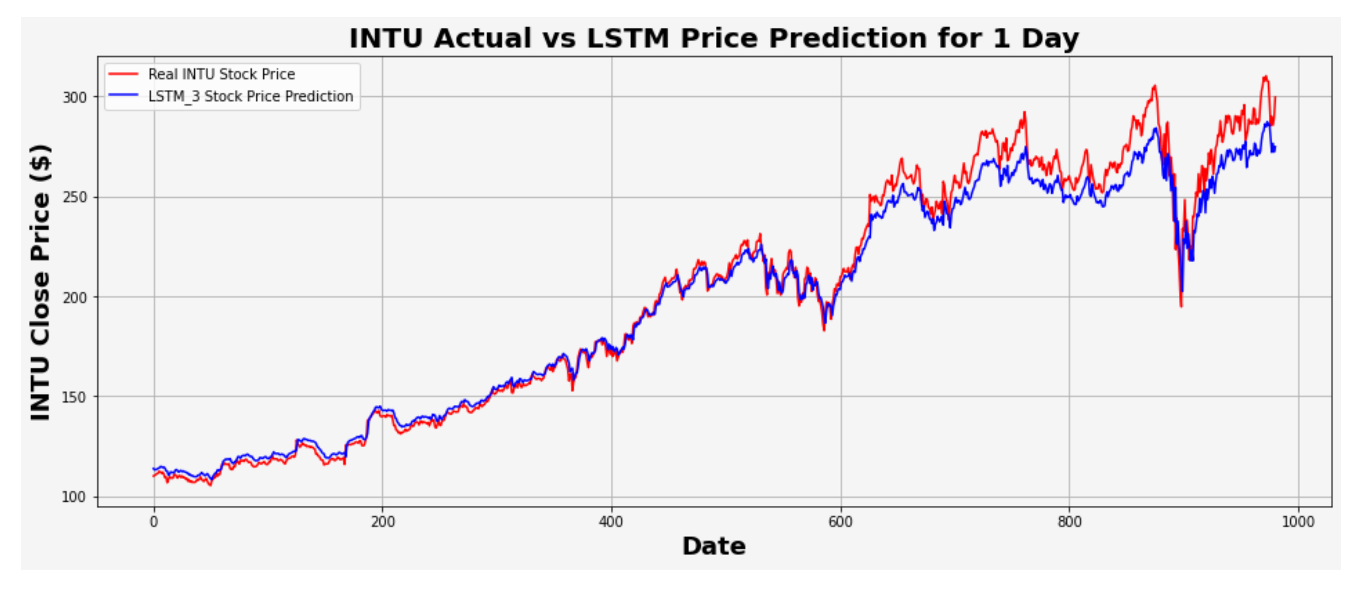
GRU establishes its superiority in all time intervals in the case of the INTU dataset. Figure 23, Figure 24 and Figure 25 represent the actual vs. predicted value curves of a one-day interval, Figure 26, Figure 27 and Figure 28 represent the curves of a three-day interval, and Figure 29, Figure 30 and Figure 31 represents the curves of a five-day interval. The values of performance metrics are summarized in the

Table 10. Performance comparison of INTU one-day interval.

Model	${\mathit{R}}^2$	MAE	MAPE	RMSE
RNN	0.98555	5.26118	2.34914	7.32498
LSTM	0.98046	6.20282	2.78882	8.51910
GRU	0.98983	3.70209	1.64523	6.14465

,

Table 11. Performance comparison of INTU three-day interval.

Model	${\mathit{R}}^2$	MAE	MAPE	RMSE
RNN	0.94280	10.65475	4.46536	14.21290
LSTM	0.97453	6.85287	2.97133	9.48472
GRU	0.98988	3.91155	1.82053	5.97660

and

Table 12. Performance comparison of INTU five-day interval.

Model	${\mathit{R}}^2$	MAE	MAPE	RMSE
RNN	0.90405	13.57545	5.65341	17.83176
LSTM	0.96641	7.83521	3.41306	10.55002
GRU	0.98227	4.99038	2.31463	7.66498

for one-day, three-day, and five-day intervals, respectively.

4.4. Performance Analysis

Based on the results of the previous three subsections, it is evident that RNN is outperformed by LSTM and GRU in stock price prediction. The reason is that both LSTM and GRU are advanced versions of traditional RNN and provide more controlling knobs, which control the flow input based on the training weights. This gives LSTM and GRU more flexibility to control the output and thus improve the performance. Another reason is that RNN suffers from the vanishing gradient problem, which may cause RNN to stop being trained if the learning rate is too low. However, with the help of update gate, forget gate, and reset gate, LSTM and GRU can avoid this problem [42]. Moreover, in terms of highly fluctuating data (INTU), although LSTM can closely identify the trend ($R^2$ value is close to GRU), it produces very large errors compared to GRU for all timeframes. Furthermore, in our research, we applied our methods on three types of data (highly fluctuating, moderately fluctuating, and slightly fluctuating) where highly fluctuating data are of the non-stationary type. High $R^2$ value indicates better fit to the regression model, and thus better prediction can be made, which is our ultimate goal in this research work. For non-stationary-type data in our analysis, we achieved very high rate of $R^2$ value for every method in each time frame, which is shown in Table 10, Table 11, and Table 12. It can therefore be said our methods are robust to non- stationary data as well.

5. Conclusions and Future Works

Investors in the stock market are always searching for new techniques to outperform the stock market and make a good profit. Researchers around the world continue to conduct research in this area to meet the demand of the investors. In this research, we have tried to analyze the performance of different versions of recurrent neural networks (simple RNN, LSTM, and GRU) in time series analysis in the domain of stock price forecasting. We have experimented with three different types of stocks. One stock’s price fluctuates very little, another one’s price fluctuates moderately, and the other one has a very high fluctuation. We have also considered three timeframes to identify how these RNN models behave in each of these situations. GRU performs better in terms of slightly fluctuating and highly fluctuating data, while LSTM produces better results when the pattern is not too flat or too sharp. From the results, we can say that both LSTM and GRU give better performance than RNN because RNN suffers from vanishing gradient problem and also has less control on the input and output. Investors should therefore try updated versions of RNN instead of traditional RNN to predict stock price movement. Investors can also have up to 5 days to figure out their buying and selling points. On the other hand, policymakers can use this model to monitor the stock market and take any actions to control the market if there is any chance of chaos in it. More interestingly, our model can also be applied in the foreign exchange currency market as both markets are similar in nature.

In the future, an application can be built that can take the historical data of stock as input, and the user will have the options to predict future price directly from the application. We also plan to do the prediction for other timeframes (such as 7 days, 10 days, 14 days, etc.) as well. Moreover, we will explore how the prediction works when a combination of multiple deep learning models is used.

References

1. Statista. Largest Stock Exchange Operators Worldwide as of January 2021, by Market Capitalization of Listed Companies (in Trillion U.S. dollars). 2021. Available online: https://www.statista.com/statistics/270126/largest-stock-exchange-operators-by-market-capitalization-of-listed-companies (accessed on 24 April 2021).
2. Hossain, E.; Shariff, M.A.U.; Hossain, M.S.; Andersson, K. A Novel Deep Learning Approach to Predict Air Quality Index. In Proceedings of the International Conference on Trends in Computational and Cognitive Engineering, Parit Raja, Malaysia, 21–22 October 2021. [Google Scholar]
3. Saiful Islam, M.; Hossain, E. Foreign Exchange Currency Rate Prediction using a GRU-LSTM Hybrid Network. Available online: https://www.sciencedirect.com/science/article/pii/S2666222120300083 (accessed on 10 July 2021).
4. Islam, M.; Hossain, E.; Rahman, A.; Hossain, M.S.; Andersson, K. A review on recent advancements in forex currency prediction. Algorithms 2020, 13, 186. [Google Scholar] [CrossRef]
5. LeCun, Y.; Bengio, Y.; Hinton, G. Deep learning. Nature 2015, 521, 436–444. [Google Scholar] [CrossRef]
6. Sun, Y.; Wang, X.; Tang, X. Deep learning face representation from predicting 10,000 classes. In Proceedings of the IEEE Conference on Computer Vision and Pattern Recognition, Columbus, OH, USA, 23–28 June 2014; pp. 1891–1898. [Google Scholar]
7. Yong, B.X.; Rahim, M.R.A.; Abdullah, A.S. A stock market trading system using deep neural network. In Proceedings of the Asian Simulation Conference, Melaka, Malaysia, 27–29 August 2017; pp. 356–364. [Google Scholar]
8. Fama, E.F. Efficient Capital Markets: A Review of Theory and Empirical Work. J. Financ. 1970, 25, 383–417. [Google Scholar] [CrossRef]
9. Fama, E.F. Efficient Capital Markets: II. J. Financ. 1991, 46, 1575–1617. [Google Scholar] [CrossRef]
10. Ferreira, P.; Pereira, E.J.; Pereira, H.B. From Big Data to Econophysics and Its Use to Explain Complex Phenomena. J. Risk Financ. Manag. 2020, 13, 153. [Google Scholar] [CrossRef]
11. Wu, D.; Wang, X.; Wu, S. A Hybrid Method Based on Extreme Learning Machine and Wavelet Transform Denoising for Stock Prediction. Entropy 2021, 23, 440. [Google Scholar] [CrossRef] [PubMed]
12. Ecer, F.; Ardabili, S.; Band, S.S.; Mosavi, A. Training Multilayer Perceptron with Genetic Algorithms and Particle Swarm Optimization for Modeling Stock Price Index Prediction. Entropy 2020, 22, 1239. [Google Scholar] [CrossRef]
13. Vințe, C.; Ausloos, M.; Furtună, T.F. A Volatility Estimator of Stock Market Indices Based on the Intrinsic Entropy Model. Entropy 2021, 23, 484. [Google Scholar] [CrossRef] [PubMed]
14. Abraham, C.M.; Elayidom, M.S.; Santhanakrishnan, T. Analysis and Design of an Efficient Temporal Data Mining Model for the Indian Stock Market. In Emerging Technologies in Data Mining and Information Security; Springer: Berlin/Heidelberg, Germany, 2019; pp. 615–628. [Google Scholar]
15. Fischer, T.; Krauss, C. Deep learning with long short-term memory networks for financial market predictions. Eur. J. Oper. Res. 2018, 270, 654–669. [Google Scholar] [CrossRef] [Green Version]
16. Parmar, I.; Agarwal, N.; Saxena, S.; Arora, R.; Gupta, S.; Dhiman, H.; Chouhan, L. Stock market prediction using Machine Learning. In Proceedings of the 2018 First International Conference on Secure Cyber Computing and Communication (ICSCCC), Jalandhar, India, 15–17 December 2018; pp. 574–576. [Google Scholar]
17. Engle, R.F.; Granger, C. Time-series econometrics: Cointegration and autoregressive conditional heteroskedasticity. In Advanced information on the Bank of Sweden Prize in Economic Sciences in Memory of Alfred Nobel; Royal Swedish Academy of Sciences: Stockholm, Sweden, 2003; pp. 1–30. [Google Scholar]
18. Cakra, Y.E.; Trisedya, B.D. Stock price prediction using linear regression based on sentiment analysis. In Proceedings of the 2015 International Conference on Advanced Computer Science and Information Systems (ICACSIS), Depok, Indonesia, 10–11 October 2015. [Google Scholar]
19. Afeef, M.; Ihsan, A.; Zada, H. Forecasting stock prices through univariate ARIMA modeling. NUML Int. J. Bus. Manag. 2018, 13, 130–143. [Google Scholar]
20. Nabipour, M.; Nayyeri, P.; Jabani, H.; Mosavi, A.; Salwana, E. Deep learning for stock market prediction. Entropy 2020, 22, 840. [Google Scholar] [CrossRef] [PubMed]
21. Börjesson, L.; Singull, M. Forecasting Financial Time Series through Causal and Dilated Convolutional Neural Networks. Entropy 2020, 22, 1094. [Google Scholar] [CrossRef]
22. Long, W.; Lu, Z.; Cui, L. Deep learning-based feature engineering for stock price movement prediction. Knowledge-Based Syst. 2019, 164, 163–173. [Google Scholar] [CrossRef]
23. Fadlalla, A.; Lin, C.H. An analysis of the applications of neural networks in finance. Interfaces 2001, 31, 112–122. [Google Scholar] [CrossRef]
24. Thakkar, A.; Chaudhari, K. A comprehensive survey on portfolio optimization, stock price and trend prediction using particle swarm optimization. Arch. Comput. Methods Eng. 2020, 28, 2133–2164. [Google Scholar] [CrossRef]
25. Maqbool, N.; Hameed, W.; Habib, M. Impact of political influences on stock returns. Int. J. Multidiscip. Sci. Publ. (IJMSP) 2018, 1, 1–6. [Google Scholar]
26. Spanos, G.; Angelis, L. The impact of information security events to the stock market: A systematic literature review. Comput. Secur. 2016, 58, 216–229. [Google Scholar] [CrossRef]
27. Baker, S.R.; Bloom, N.; Davis, S.J.; Kost, K.J. Policy News and Stock Market Volatility; Technical Report; National Bureau of Economic Research: Cambridge, MA, USA, 2019. [Google Scholar]
28. Christiano, L.; Ilut, C.L.; Motto, R.; Rostagno, M. Monetary Policy and Stock Market Booms; Technical Report; National Bureau of Economic Research: Cambridge, MA, USA, 2010. [Google Scholar]
29. Prajapati, P.; Chaudhari, K. KBC: Multiple Key Generation using Key Block Chaining. Procedia Comput. Sci. 2020, 167, 1960–1969. [Google Scholar] [CrossRef]
30. Chaudhari, K.; Prajapati, P. Parallel DES with Modified Mode of Operation. In Intelligent Communication, Control and Devices; Springer: Berlin/Heidelberg, Germany, 2020; pp. 819–831. [Google Scholar]
31. Goodfellow, I.; Bengio, Y.; Courville, A.; Bengio, Y. Deep Learning; MIT Press: Cambridge, UK, 2016; Volume 1. [Google Scholar]
32. Connor, J.T.; Martin, R.D.; Atlas, L.E. Recurrent neural networks and robust time series prediction. IEEE Trans. Neural Netw. 1994, 5, 240–254. [Google Scholar] [CrossRef] [Green Version]
33. Mei, F.; Chen, H.; Lei, Y. Blind Recognition of Forward Error Correction Codes Based on Recurrent Neural Network. Sensors 2021, 21, 3884. [Google Scholar] [CrossRef]
34. Mateus, B.C.; Mendes, M.; Farinha, J.T.; Cardoso, A.M. Anticipating Future Behavior of an Industrial Press Using LSTM Networks. Appl. Sci. 2021, 11, 6101. [Google Scholar] [CrossRef]
35. Sagheer, A.; Hamdoun, H.; Youness, H. Deep LSTM-Based Transfer Learning Approach for Coherent Forecasts in Hierarchical Time Series. Sensors 2021, 21, 4379. [Google Scholar] [CrossRef] [PubMed]
36. Xu, L.; Hu, J. A Method of Defect Depth Recognition in Active Infrared Thermography Based on GRU Networks. Appl. Sci. 2021, 11, 6387. [Google Scholar] [CrossRef]
37. Liu, C.; Yang, X.; Peng, S.; Zhang, Y.; Peng, L.; Zhong, R.Y. Spark Analysis Based on the CNN-GRU Model for WEDM Process. Micromachines 2021, 12, 702. [Google Scholar] [CrossRef] [PubMed]
38. Honda Motor Company (HMC) Stock Price. 2021. Available online: https://finance.yahoo.com/quote/HMC?p=HMC&.tsrc=fin-srch (accessed on 24 April 2021).
39. Oracle Corporation (ORCL) Stock Price. 2021. Available online: https://finance.yahoo.com/quote/ORCL?p=ORCL&.tsrc=fin-srch (accessed on 24 April 2021).
40. Intuit Inc. (INTU) Stock Price. 2021. Available online: https://finance.yahoo.com/quote/INTU?p=INTU&.tsrc=fin-srch (accessed on 24 April 2021).
41. Swamidass, P.M. (Ed.) Mean Absolute Percentage Error (MAPE). In Encyclopedia of Production and Manufacturing Management; Springer: Boston, MA, USA, 2000; p. 462. [Google Scholar] [CrossRef]
42. Graves, A. Long short-term memory. In Supervised Sequence Labelling with Recurrent Neural Networks; Springer: Berlin/Heidelberg, Germany, 2012; pp. 37–45. [Google Scholar]
Figure 1. Simple RNN Architecture.
Algorithms 14 00251 g001
Figure 2. A single cell LSTM architecture.
Algorithms 14 00251 g002
Figure 3. A general architecture of a single GRU cell.
Algorithms 14 00251 g003
Figure 4. System architecture of stock price prediction for different frequency domains.
Algorithms 14 00251 g004
Figure 5. HMC actual vs. RNN predicted for one-day interval.
Algorithms 14 00251 g005
Figure 6. HMC actual vs. LSTM predicted for one-day interval.
Algorithms 14 00251 g006
Figure 7. HMC actual vs. GRU predicted for one-day interval.
Algorithms 14 00251 g007
Figure 8. HMC actual vs. RNN predicted for three-day interval.
Algorithms 14 00251 g008
Figure 9. HMC actual vs. LSTM predicted for three-day interval.
Algorithms 14 00251 g009
Figure 10. HMC actual vs. GRU predicted for three-day interval.
Algorithms 14 00251 g010
Figure 11. HMC actual vs. RNN predicted for five-day interval.
Algorithms 14 00251 g011
Figure 12. HMC actual vs. LSTM predicted for five-day interval.
Algorithms 14 00251 g012
Figure 13. HMC actual vs. GRU predicted for five-day interval.
Algorithms 14 00251 g013
Figure 14. ORCL actual vs. RNN predicted for one-day interval.
Algorithms 14 00251 g014
Figure 15. ORCL actual vs. LSTM predicted for one-day interval.
Algorithms 14 00251 g015
Figure 16. ORCL actual vs. GRU predicted for one-day interval.
Algorithms 14 00251 g016
Figure 17. ORCL actual vs. RNN predicted for three-day interval.
Algorithms 14 00251 g017
Figure 18. ORCL actual vs. LSTM predicted for three-day interval.
Algorithms 14 00251 g018
Figure 19. ORCL actual vs. GRU predicted for three-day interval.
Algorithms 14 00251 g019
Figure 20. ORCL actual vs. RNN predicted for five-day interval.
Algorithms 14 00251 g020
Figure 21. ORCL actual vs. LSTM predicted for five-day interval.
Algorithms 14 00251 g021
Figure 22. ORCL actual vs. GRU predicted for five-day interval.
Algorithms 14 00251 g022
Figure 23. INTU actual vs. RNN predicted for one-day interval.
Algorithms 14 00251 g023
Figure 24. INTU actual vs. LSTM predicted for one-day interval.
Algorithms 14 00251 g024
Figure 25. INTU actual vs. GRU predicted for one-day interval.
Algorithms 14 00251 g025
Figure 26. INTU actual vs. RNN predicted for three-day interval.
Algorithms 14 00251 g026
Figure 27. INTU actual vs. LSTM predicted for three-day interval.
Algorithms 14 00251 g027
Figure 28. INTU actual vs. GRU predicted for three-day interval.
Algorithms 14 00251 g028
Figure 29. INTU actual vs. RNN predicted for five-day interval.
Algorithms 14 00251 g029
Figure 30. INTU actual vs. LSTM predicted for five-day interval.
Algorithms 14 00251 g030
Figure 31. INTU actual vs. GRU predicted for five-day interval.
Algorithms 14 00251 g031