Defuzzify Imprecise Numbers Using the Mellin Transform and the Trade-Off between the Mean and Spread

Abstract

Uncertainty or vagueness is usually used to reflect the limitations of human subjective judgment on practical problems. Conventionally, imprecise numbers, e.g., fuzzy and interval numbers, are used to cope with such issues. However, these imprecise numbers are hard for decision-makers to make decisions, and, therefore, many defuzzification methods have been proposed. In this paper, the information of the mean and spread/variance of imprecise data are used to defuzzify imprecise data via Mellin transform. We illustrate four numerical examples to demonstrate the proposed methods, and extend the method to the simple additive weighting (SAW) method. According to the results, our method can solve the problem of the inconsistency between the mean and spread, compared with the center of area (CoA) and bisector of area (BoA), and is easy and efficient for further applications.

1. Introduction

As we know, the real world is imperfect, imprecise, and uncertain. Hence, many theories and approaches, e.g., fuzzy sets, rough sets, and interval sets, have been proposed to reflect the vagueness of the real world. To reflect the human’s subjective uncertainty of linguistics, Professor Zadeh used fuzzy numbers to capture the uncertainty and the membership function to be the corresponding weights [1]. Usually, a fuzzy number is represented by a triangular fuzzy number (a₁, a₂, a₃), where a₁, a₂, and a₃ are the left, center, and right values of a fuzzy number, respectively. Indeed, we can use alternative forms, e.g., trapezoidal or Gaussian, to present fuzzy numbers.

However, in most practical situations, we still hope the information for decision-making is clear and crisp. Therefore, many defuzzification methods are proposed and used to transform imprecise values, e.g., interval or fuzzy numbers, into crisp values for decision-making. Note that defuzzifying imprecise data means using some functions to transform fuzzy or interval numbers into crisp values. Since imprecise data analysis, no matter interval or fuzzy numbers, is popular in many fields, e.g., multiobjective programming [2,3,4], data envelopment analysis (DEA) [5,6,7], and decision sciences [8,9,10], the defuzzification of imprecise numbers is a critical topic.

The problem of defuzzifying interval numbers is similar to that of defuzzifying fuzzy numbers. The main difference is that the y-axis of fuzzy numbers denotes the membership function, but the y-axis of interval numbers is the probability density function (pdf). The authors of [11] first proposed the concept of ranking fuzzy numbers using the mean and spread. However, it is inefficient to determine the better fuzzy number or interval data when one has a higher mean and a higher spread. Although the concept of coefficient of variance (CV) was provided in [12] to cope with the problem of inconsistency, it fails when there are crisp values, and it is hard to apply to follow-up multiple attribute decision-making (MADM) applications, such as simple additive weighting (SAW) or weight product method (WPM), due to the fact the original unit is changed. Hence, an easy and efficient algorithm to defuzzify imprecise numbers is a critical issue for practical applications.

In this paper, we first find the mean and spread of imprecise numbers via the Mellin transformation. Then, we derive the trade-off coefficient between the mean and spread. Finally, we develop the preference relation of imprecise numbers to rank them. In addition, we use four examples to demonstrate our concepts and extend our method to choose the best alternative using the SAW method. Based on the numerical results, our method can handle the problem of the inconsistency between the mean and the spread with respect to the center of area (CoA) and the bisector of area (BoA), and can be easily used in further applications.

The rest of this paper is organized as follows. Section 2 states the problem of the inconsistency between the mean and the spread. Section 3 derives the relation between the mean and the spread according to the utility theory. The detail of the Mellin transform is presented in Section 4. Four numerical examples are used in Section 5 to demonstrate our concept. Discussion is presented in Section 6, and the final section presents conclusions.

2. Statement of the Problem

Assume there are two alternatives, $A_i$ and $A_j$, and their means and spreads are ${\mu }_i$, ${\mu }_j$, and ${\sigma }_i$, ${\sigma }_j$, respectively. According to [10], the rules for ranking fuzzy numbers is $A_i\succ A_j$ if ${\mu }_i>{\mu }_j$ or $A_i\succ A_j$ if ${\mu }_i={\mu }_j$ and ${\sigma }_i<{\sigma }_j$. However, if we assume there are two imprecise numbers with uniform distributions, then the rules seem incorrect when there is a smaller mean and a smaller spread, as in Figure 1.

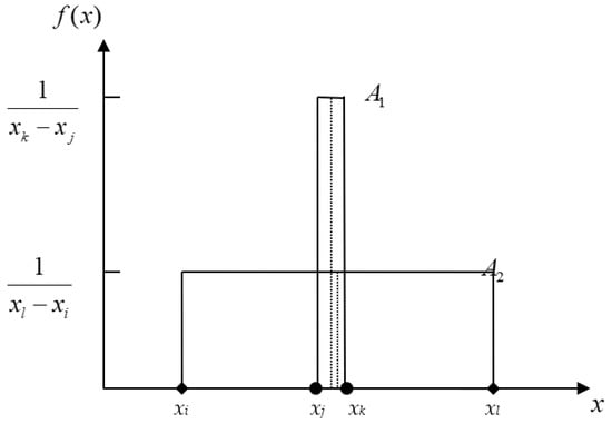
Figure 1. The conflicting situation in precise data.

It is intuitive for a decision-maker to prefer $A_1$ over $A_2$, even though $A_2$ has a higher mean than $A_1$. That being said, the higher mean does not necessarily have the higher ranking order if the spread is too large, i.e., the mean and the spread comprise the trade-off relation. This situation is also called risk premium (RP), which represents the additional compensation required for assuming a higher risk, and is usually discussed in economic and financial management.

In addition, [12] proposed another criterion, called the CV index, to improve Lee and Li’s method [11] according to the following equation:

$$CV=\frac{\sigma }{\left|\mu \right|}$$

(1)

where $\sigma$ denotes the spread and $\mu$ denotes the mean.

However, it is clear that the CV index fails when there are crisp values or the mean is zero. In addition, another shortcoming is that the result is difficult to interpret because the unit has changed. Hence, many researchers provided different methods to efficiently rank fuzzy numbers, e.g., [13,14,15,16,17], or interval numbers, e.g., [16,17].

Another practical issue is that ranking imprecise numbers is not enough for further applications. A decision-maker might like to derive the crisp values of alternatives [18]. Surely, plenty of defuzzification methods have been proposed to efficiently derive the crisp values from imprecise numbers, e.g., the center of sums method, the CoA method, the BoA method, the weighted average method, and different kinds of maxima methods. However, none of them can handle all the considered situations here, and we will compare our method with CoA and BoA to justify the proposed method. Here, we incorporate the concept of risk premium into our method and derive the trade-off coefficient between the mean and spread to rank and defuzzify imprecise numbers.

3. A Trade-Off between the Mean and Spread

According to utility theory, it is intuitive that a higher mean (${\mu }_A$) has a higher utility ($u(A)$) and a lower spread (${\sigma }_A$), correspondingly, has a higher utility. For simplicity, we assume the equations are linear as:

$$u(A)=a+b{\mu }_A$$

(2)

$$u(A)=c-d{\sigma }_A$$

(3)

and

$${\frac{du}{d\mu }}_A>0, \frac{du}{d{\sigma }_A}<0$$

Next, we derive the relationship between the mean and spread according to our assumptions. Let two points be ${\mu }_{A_1}$ and ${\mu }_{A_2},$ then $u(A_1),$ $u(A_2)$, ${\sigma }_{A_1},$ and ${\sigma }_{A_2}$ can be derived by Equations (2) and (3) to form the relationship between ${\mu }_A$ and ${\sigma }_A$, as shown in Figure 2.

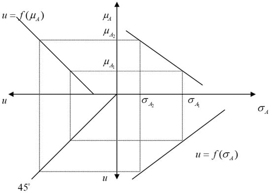
Figure 2. The relationship between the mean and the spread.

According to Figure 2, we know that having an alternative with a larger spread is the same as having a smaller mean and vice versa. Hence, the trade-off between the mean and the spread can be defined as:

$$\Delta {\mu }_A=\theta \Delta {\sigma }_A$$

(4)

where $\theta <0$ is an indifference ratio between the mean and the spread.

Next, we develop a criterion to incorporate the mean and the spread according to Equation (4). This is because if we can transform the spread to the mean, we can easily compare any imprecise data using the rule for the higher mean with the higher ranking order. Based on this concept, we can transform the difference between the spreads into the difference between the means and let:

$$\Delta {\mu }_A={\mu }_{\Delta }(A_1,A_2)={\mu }_{A_1}-{\mu }_{A_2}$$

(5)

$$\Delta {\sigma }_A={\sigma }_{\Delta }(A_1,A_2)={\sigma }_{A_2}-{\sigma }_{A_1}$$

(6)

Then, we can obtain the equation to be the criterion to rank the imprecise data as:

$$\Delta {\mathrm{\Psi }}_A=\mathrm{\Psi }(A_1,A_2)={\mu }_{\Delta }(A_1,A_2)+\lambda {\sigma }_{\Delta }(A_1,A_2)$$

(7)

where $\Delta {\mathrm{\Psi }}_A$ denotes the preference difference between two imprecise numbers and $\lambda$ = $-\theta$ indicates the trade-off ratio between the mean and the spread.

Equation (7) indicates that the grades of the utility in $A_1$ are superior to $A_2$, so we can conclude that

$$\Delta {\mathrm{\Psi }}_A>0, \mathrm{if} A_1\succ A_2$$

(8)

$$\Delta {\mathrm{\Psi }}_A<0, \mathrm{if} A_1\prec A_2$$

(9)

$$\Delta {\mathrm{\Psi }}_A=0, \mathrm{if} A_1\approx A_2$$

(10)

As the mean and spread are monotone functions, it is obvious that $\Delta {\mathrm{\Psi }}_A$ satisfies the transitive axiom (i.e., if $A_1\succ A_2$ and $A_2\succ A_3$, then $A_1\succ A_3$). In addition, our simulation indicates $\theta$ is approximately equal to −0.25, and the method of our experiment is listed in Appendix A.

Let us consider the defuzzifying problem of the proposed method as follows. Let $A_i$ be a status quo alternative. The defuzzifying value of $A_i$ is its ${\mu }_{A_1}$, and the defuzzifying value of $A_j$ can be derived as:

$$A_j={\mu }_{A_1}+\lambda {\sigma }_{\Delta }(A_1,A_2)$$

(11)

In addition, this paper uses the Mellin transform to calculate the mean and spread/variance in any distribution quickly. Next, we describe details of the Mellin transform, and link it to the nth moment to calculate the mean and spread.

4. An Application of the Mellin Transform

Given a random variable, $x\in R^{+},$ the Mellin transform, $M(s),$ of a pdf, $f(x)$, can be defined as:

$$M\{f(x);s\}=M(s)={\displaystyle {\int }_0^{\infty }f(x)x^{s-1}dx}$$

(12)

Let $h$ be a measurable function on $\mathit{ℝ}$ into $\mathit{ℝ}$ and $Y=h(x)$ is a random variable. Then, some properties of the Mellin transform can be described, as shown in Table 1. For example, if $Y=ax,$ then the scaling property can be expressed as:

$$M\{f(ax);s\}={\displaystyle {\int }_0^{\infty }f(ax)x^{s-1}dx}=a^{-s}{\displaystyle {\int }_0^{\infty }f(ax){(ax)}^{s-1}}=a^{-s}M(s)$$

(13)

Table 1. The properties of the Mellin transform.

Properties of Mellin Transform	$\mathit{Y}=\mathit{h}(\mathit{x})$	$\mathit{M}(\mathit{s})$
Scaling property	$ax$	$a^{-s}M(s)$
Multiplication by $x^a$	$x^{a}f(x)$	$M(s+a)$
Rising to a real power	$f(x^a)$	$a^{-1}M(\frac{s}{a}),a>0$
Inverse	$x^{-1}f(x^{-1})$	$M(1-s)$
Multiplication by $lnx$	$lnxf(x)$	$\frac{d}{ds}M(s)$
Derivative	$\frac{d^k}{d{s}^k}f(x)$	$\frac{\mathrm{\Gamma }(s)}{\mathrm{\Gamma }(s-k)}$

Given a continuous non-negative random variable, X, the nth moment of X is denoted by $E(X^n)$ and is defined as:

$$E(X^n)={\displaystyle {\int }_0^{\infty }{x}^{n}f(x)dx}$$

(14)

For n = 1, the mean of X can be expressed as:

$$E(X)={\displaystyle {\int }_0^{\infty }xf(x)dx}$$

(15)

and the variance of X can be calculated by:

$${\sigma }_x^2=E(X^2)-{[E(X)]}^2$$

(16)

Since the relation between the nth moment and the Mellin transform of X can be linked by:

$$E(X^n)={\displaystyle {\int }_0^{\infty }{x}^{(n+1)-1}f(x)dx}=M\{f(x);n+1\}$$

(17)

then the mean and the variance of X can be calculated by:

$$E(X)=M\{f(x);2\}$$

(18)

$${\sigma }_x^2=M\{f(x);3\}-{\left\{M\right\{f(x);2\left\}\right\}}^2$$

(19)

According to Equations (18) and (19), we can quickly calculate the mean and the spread in any distribution. In practice, the uniform, the triangular, and the trapezoidal distribution are usually used, and their Mellin transforms are summarized as shown in Table 2. More Mellin transforms in various probabilistic density functions can be found in [19].

Table 2. Mellin transform of some probability density functions.

Distribution	Parameters	M(s)
Uniform	$UNI(a,b)$	$\frac{b^s-a^s}{s(b-a)}$
Triangular	$TRI(l,m,u)$	$\frac{2}{(u-l)s(s+1)}[\frac{u(u^s-m^s)}{(u-m)}-\frac{l(m^s-l^s)}{(m-l)}]$
Trapezoidal	$TRA(a,b,c,d)$	$\frac{2}{(c+d-b-a)s(s+1)}[\frac{(d^{s+1}-c^{s+1})}{(d-c)}-\frac{(b^{s+1}-a^{s+1})}{(b-a)}]$

Based on Table 2, the mean and spread values can be efficiently derived by calculating $M(2)$ and $M(3)$. Then, we can rank and defuzzify imprecise data using Equation (7). The following section uses four numerical examples to show the detailed procedures of the proposed method.

5. Numerical Examples

In this section, we demonstrate four examples to show how our method ranks imprecise data. The first three examples illustrate the way to rank various imprecise data. The last example demonstrates our approach to extending to the simple additive weighting method. The Mellin transform derives the values of the mean and spread, and the preference of objects is obtained by incorporating the variance into the mean value.

Example 1.

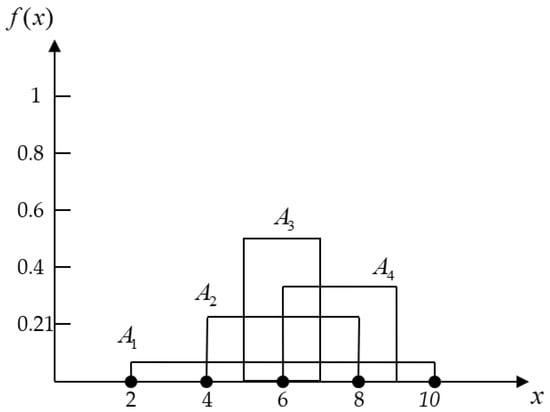
Let four alternatives using imprecise data be used to measure the preference where we do not know any information about our alternatives (i.e., assuming they have uniform distribution). Their imprecise preferences are A₁ = (2, 10), A₂ = (4, 8), A₃ = (5, 7), and A₄ = (6, 9), and these probability density functions are represented in Figure 3.

Figure 3. The probability density function in the first example.

According to the Mellin transform, we can obtain:

$$\begin{gathered} E(A_1)=6.0, {\sigma }_{A_1}=2.3094 \\ E(A_2)=6.0, {\sigma }_{A_2}=1.1547 \\ E(A_3)=6.0, {\sigma }_{A_3}=0.5774 \\ E(A_4)=7.5, {\sigma }_{A_4}=0.8660 \end{gathered}$$

then the differences in the alternatives’ total mean can be calculated as:

$$\begin{gathered} \mathrm{\Psi }(A_1,A_2)={\mu }_{\Delta }(A_1,A_2)+\lambda {\sigma }_{\Delta }(A_1,A_2)=0+0.25\times (1.1547-2.3094)=-0.2887<0 \\ \mathrm{\Psi }(A_1,A_3)={\mu }_{\Delta }(A_1,A_3)+\lambda {\sigma }_{\Delta }(A_1,A_3)=0+0.25\times (0.5774-2.3094)=-0.4330<0 \\ \mathrm{\Psi }(A_1,A_4)={\mu }_{\Delta }(A_1,A_4)+\lambda {\sigma }_{\Delta }(A_1,A_4)=-1.5+0.25\times (0.8660-2.3094)=-1.8609<0 \end{gathered}$$

Based on the above result, we can conclude the ranking result is $A_4\succ A_3\succ A_2\succ A_1$. We can set A₁ as the status quo alternative and defuzzify other alternatives. The result is compared with CoA and Boa and presented, as shown in Table 3.

Table 3. The comparison of defuzzifying approaches in Example 1.

Methods	A1	A2	A3	A4	Rank
CoA	6	6	6	7.5	$A_4\succ A_3\approx A_2\approx A_1$
BoA	6	6	6	7.5	$A_4\succ A_3\approx A_2\approx A_1$
Proposed	6 (status quo)	6.29	6.43	7.86	$A_4\succ A_3\succ A_2\succ A_1$

Example 2.

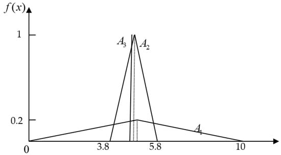
Given two imprecise data with triangular distributions, A₁ = (0, 6, 10) and A₂ = (3.8, 4.8, 5.8), and a crisp value A₃ = 4.6, to present the measurement of the preference in A₁, A₂, and A₃. Their probability density functions are listed in Figure 4.

Figure 4. The probability density function in the second example.

By using the Mellin transform,

$$\begin{gathered} E(A_1)=5.0, {\sigma }_{A_1}=2.0412 \\ E(A_2)=4.8, {\sigma }_{A_2}=0.4082 \\ E(A_3)=4.6, {\sigma }_{A_3}=0 \end{gathered}$$

then the differences in the alternative’s total mean can be calculated as:

$$\begin{gathered} \mathrm{\Psi }(A_1,A_2)={\mu }_{\Delta }(A_1,A_2)+\lambda {\sigma }_{\Delta }(A_1,A_2)=0.2+0.25\times (0.4082-2.0412)=-0.2083<0 \\ \mathrm{\Psi }(A_2,A_3)={\mu }_{\Delta }(A_2,A_3)+\lambda {\sigma }_{\Delta }(A_2,A_3)=0.2+0.25\times (0-0.4082)=-0.0980<0 \end{gathered}$$

The above result indicates that the preference relation is $A_3\succ A_2\succ A_1$, where A₃ is the best choice. Then, we can compare the proposed method with CoA and Boa, as shown in Table 4.

Table 4. The comparison of defuzzifying approaches in Example 2.

Methods	A1	A2	A3	Rank
CoA	5.33	4.59	4.6	$A_1\succ A_3\succ A_2$
BoA	5.5	4.6	4.6	$A_1\succ A_3\approx A_2$
Proposed	4.6	4.8 (status quo)	4.9	$A_3\succ A_2\succ A_1$

Example 3.

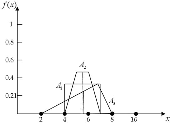
Assume three alternatives (A₁, A_2, and A₃) using interval data to measure the preference rating, and of these alternatives, A₂ and A₃ are known to have trapezoidal and triangular distributions, respectively. Their scores are A₁ = (4, 7), A₂ = (4, 5, 6, 7), and A₃ = (2, 7, 8), respectively, and the probability density functions are described in Figure 5.

Figure 5. The probability density function in the third example.

By using the Mellin transform, the mean and the spread can be calculated as:

$$\begin{gathered} E(A_1)=5.5, {\sigma }_{A_1}=0.8660 \\ E(A_2)=5.5, {\sigma }_{A_2}=0.4167 \\ E(A_3)=5.67, {\sigma }_{A_3}=1.2329 \end{gathered}$$

then the differences in the alternatives’ total mean can be calculated as:

$$\begin{gathered} \mathrm{\Psi }(A_1,A_2)={\mu }_{\Delta }(A_1,A_2)+\lambda {\sigma }_{\Delta }(A_1,A_2)=0+0.25\times (0.4167-0.8660)=-0.1378<0 \\ \mathrm{\Psi }(A_1,A_3)={\mu }_{\Delta }(A_1,A_3)+\lambda {\sigma }_{\Delta }(A_1,A_3)=-0.1+0.25\times (1.2329-0.8660)=-0.008<0 \\ \mathrm{\Psi }(A_2,A_3)={\mu }_{\Delta }(A_2,A_3)+\lambda {\sigma }_{\Delta }(A_2,A_3)=-0.17+0.25\times (1.2329-0.4167)=0.0341>0 \end{gathered}$$

The above result indicates that $A_2\succ A_3\succ A_1$, and we can compare the proposed method with CoA and Boa, as shown in Table 5.

Table 5. The comparison of defuzzifying approaches in Example 3.

Methods	A1	A2	A3	Rank
CoA	5.5	5.5	5.67	$A_3\succ A_1\approx A_2$
BoA	5.5	5.5	5.9	$A_3\succ A_1\approx A_2$
Proposed	5.5 (status quo)	5.64	5.51	$A_2\succ A_3\succ A_1$

Example 4.

In order to extend to further applications in MADM, we demonstrate a way to employ the SAW method using our concept. The SAW method can be expressed as:

$$V(A_i)=V_i={\displaystyle \sum _{j=1}^n{w}_j{v}_j(x_{ij}),\begin{array}{cc}& i=1,\cdots ,m\end{array}};j=1,\dots ,n$$

(20)

where$V(A_i)$is the value function of alternative$A_i$, and$w_j$and$v_j(\cdot )$are weight and value functions of attribute$j$, respectively. After a normalization process, the value of alternative$A_i$can be rewritten as:

$$V_i={\displaystyle \sum _{j=1}^n{w}_j{r}_{ij},\begin{array}{cc}& i=1,\cdots ,m\end{array}}$$

(21)

Next, we can apply our concept to the simple additive weighting method according to follow equations:

$$\Delta V_{ik}=V_i-V_k={\displaystyle \sum _{j=1}^n{w}_j{r}_{ij}}-{\displaystyle \sum _{j=1}^n{w}_j{r}_{kj}}={\displaystyle \sum _{j=1}^n{w}_j\Delta r_{ikj}}, i,k=1,\cdots ,m;j=1,\cdots ,n$$

(22)

and let:

$$\Delta r_{ikj}={\mu }_{\Delta }(A_{ij},A_{kj})+\lambda {\sigma }_{\Delta }(A_{ij},A_{kj})$$

(23)

Then,

$$\mathrm{\Psi }(A_{ij},A_{kj})={\displaystyle \sum _{j=1}^h{w}_j{\mu }_{\Delta }(A_{ij},A_{kj})}+{\displaystyle \sum _{j=1}^h{w}_j\lambda {\sigma }_{\Delta }(A_{ij},A_{kj})}$$

(24)

when$\mathrm{\Psi }(A_{ij},A_{kj})>0$means$A_i\succ A_k$where$i,k\in [1,\dots ,m]$, and vice versa.

Assume there are three alternatives described in Table 6, where each alternative is measured using interval data. In addition, we assume these alternatives satisfy the uniform distributions.

Table 6. Data for evaluation in the fourth example.

Alternatives	$w_1=0.2$	$w_2=0.5$	$w_3=0.3$
$A_1$	[3.6, 5.8]	[4.3, 6.7]	[2.3, 5.7]
$A_2$	[2.3, 6.0]	[3.8, 4.6]	[4.8, 6.9]
$A_3$	[4.3, 6.4]	[4.7, 5.8]	[4.8, 6.2]

Next, we need to normalize all alternatives, and linear normalization is most often used in the SAW method [20]. Therefore, in this example, we normalize the interval data according to the following equation:

$$r_{ij}=[\frac{r^{-}}{r^{\ast }},\frac{r^{+}}{r^{\ast }}]$$

(25)

where $r^{-}$ and $r^{+}$ are the interval boundary, and $r^{\ast }$ is the maximum value in jth attribute. Based on Equation (20), we can normalize the interval data in Table 7.

Table 7. Data for evaluation in the fourth example after normalization.

Alternatives	$w_1=0.2$	$w_2=0.5$	$w_3=0.3$
$A_1$	[0.563, 0.906]	[0.642, 1.000]	[0.333, 0.826]
$A_2$	[0.359, 0.938]	[0.567, 0.687]	[0.696, 1.000]
$A_3$	[0.672, 1.000]	[0.701, 0.866]	[0.696, 0.899]

After this normalization process, we can calculate the differences between the alternatives’ means as follows:

$$\begin{gathered} \mathrm{\Psi }(A_1,A_2)={\displaystyle \sum _{j=1}^h{w}_j{\mu }_{\Delta }(A_{1j},A_{2j})}+{\displaystyle \sum _{j=1}^h{w}_j\lambda {\sigma }_{\Delta }(A_{1j},A_{2j})}=0.0206+0.0884-0.0846=0.0244>0 \\ \mathrm{\Psi }(A_1,A_3)={\displaystyle \sum _{j=1}^h{w}_j{\mu }_{\Delta }(A_{1j},A_{3j})}+{\displaystyle \sum _{j=1}^h{w}_j\lambda {\sigma }_{\Delta }(A_{1j},A_{3j})}=-0.0205+0.0118-0.0717=-0.0804<0 \end{gathered}$$

According to the results $A_1\succ A_2$ and $A_1\prec A_3$, and the alternative $A_3$ is the best choice.

6. Discussions

One critical issue for imprecise numbers is to rank their order and defuzzify their values. This paper focuses on imprecise data, and uses the mean and spread to defuzzify and rank data. Although the CoA and BoA are widely used to defuzzify fuzzy numbers because of their simplicity, they can obtain wrong preferences in more complicated situations. According to the utility theory, the difference between the spreads can be transformed into the difference between the means by multiplying a specific ratio. Therefore, we can develop some equations to achieve our purpose here.

Our method has several characteristics when ranking imprecise numbers based on our numerical examples. First, when imprecise numbers have the same mean, the smaller spread has the higher-ranking preference. Second, the influence of the spread to certain utilities can clearly be reflected in the results, so it is not necessary to have the higher mean indicate the higher-ranking preference if the spread is too large. However, the trade-off between the mean and the spread is not mentioned in Lee and Li’s method [10]. Third, our method is suitable for both imprecise and crisp data or mixed data. Last, our method does not change the measurement unit, and the results can be interpreted more intuitively and easily applied to further areas of research.

The main concept of our method is that the difference in the utility should be larger than zero when one preference is larger than another. We use three examples and the SAW method to demonstrate our concept. Based on the results, our methods can rank the preferences correctly. However, the correctness of the proposed method highly depends on the choice of $\theta$. Although we propose an experimental method to determine the parameter, other sophisticated ways should be considered in different applications or considerations. The choice of the parameter also provides the flexibility for decision-makers to reflect on the facing problems.

7. Conclusions

According to the probability theory, we can describe the characteristics of imprecise data depending on its mean and spread. These two criteria are also used to rank interval and fuzzy numbers. However, the mean and spread exist in a trade-off relationship, and it is not necessary to choose the alternative with the higher mean if the spread of the alternative is too large. In order to solve the problem of this inconsistency under the perspectives of the mean and the spread, the difference between the spread is transformed into the difference between the mean. According to the results of the preference difference between alternatives, we can rank the priority of the imprecise data. In addition, we also provide a method to derive the crisp value of an imprecise number.

There are several advantages to our proposed method. First, after transforming the spread, we can overcome the problem of being unable to determine the better ranking when one has a higher mean and spread. Second, no matter the imprecise data distribution, the mean and spread can quickly be calculated by the Mellin transform. Third, interpretation is easier and more intuitive because the unit is not changed. In addition, our method can be easily extended to other methods in MADM for further applications.

References

- Zadeh, L.A. Fuzzy Set Theory and Its Applications; University of California: Los Angeles, CA, USA, 1965; Volume 8, p. 338. [Google Scholar]
- Ishibuchi, H.; Tanaka, H. Multiobjective programming in optimization of the interval objective function. Eur. J. Oper. Res. 1990, 48, 219–225. [Google Scholar] [CrossRef]
- Shaocheng, T. Interval number and fuzzy number linear programmings. Fuzzy Sets Syst. 1994, 66, 301–306. [Google Scholar] [CrossRef]
- Sengupta, A.; Pal, T.K.; Chakraborty, D. Interpretation of inequality constraints involving interval coefficients and a solution to interval linear programming. Fuzzy Sets Syst. 2001, 119, 129–138. [Google Scholar] [CrossRef]
- Tavana, M.; Khalili-Damghani, K.; Arteaga, F.J.S.; Mahmoudi, R.; Hafezalkotob, A. Efficiency decomposition and measurement in two-stage fuzzy DEA models using a bargaining game approach. Comput. Ind. Eng. 2018, 118, 394–408. [Google Scholar] [CrossRef]
- Zhou, X.; Wang, Y.; Chai, J.; Wang, L.; Wang, S.; Lev, B. Sustainable supply chain evaluation: A dynamic double frontier network DEA model with interval type-2 fuzzy data. Inf. Sci. 2019, 504, 394–421. [Google Scholar] [CrossRef]
- Arana-Jiménez, M.; Sánchez-Gil, M.; Younesi, A.; Lozano, S. Integer interval DEA: An axiomatic derivation of the technology and an additive, slacks-based model. Fuzzy Sets Syst. 2021, 422, 83–105. [Google Scholar] [CrossRef]
- Akram, M.; Adeel, A. TOPSIS Approach for MAGDM Based on Interval-Valued Hesitant Fuzzy N-Soft Environment. Int. J. Fuzzy Syst. 2019, 21, 993–1009. [Google Scholar] [CrossRef]
- Tolga, A.C.; Parlak, I.B.; Castillo, O. Finite-interval-valued Type-2 Gaussian fuzzy numbers applied to fuzzy TODIM in a healthcare problem. Eng. Appl. Artif. Intell. 2020, 87, 103352. [Google Scholar] [CrossRef]
- Wu, L.; Gao, H.; Wei, C. VIKOR method for financing risk assessment of rural tourism projects under interval-valued intuitionistic fuzzy environment. J. Intell. Fuzzy Syst. 2019, 37, 2001–2008. [Google Scholar] [CrossRef]
- Lee, E.; Li, R.-J. Comparison of fuzzy numbers based on the probability measure of fuzzy events. Comput. Math. Appl. 1988, 15, 887–896. [Google Scholar] [CrossRef]
- Cheng, C.-H. A new approach for ranking fuzzy numbers by distance method. Fuzzy Sets Syst. 1998, 95, 307–317. [Google Scholar] [CrossRef]
- Ban, A.I.; Coroianu, L. Simplifying the Search for Effective Ranking of Fuzzy Numbers. IEEE Trans. Fuzzy Syst. 2014, 23, 327–339. [Google Scholar] [CrossRef]
- Chanas, S.; Zieliński, P. Ranking fuzzy interval numbers in the setting of random sets–further results. Inf. Sci. 1999, 117, 191–200. [Google Scholar] [CrossRef]
- Chanas, S.; Delgado, M.; Verdegay, J.; Vila, M. Ranking fuzzy interval numbers in the setting of random sets. Inf. Sci. 1993, 69, 201–217. [Google Scholar] [CrossRef]
- Moore, R.E. Interval Analysis; Prentice-Hall: Englewood Cliffs, NJ, USA, 1966; Volume 4, pp. 8–13. [Google Scholar]
- Sengupta, A.; Pal, T.K. On comparing interval numbers. Eur. J. Oper. Res. 2000, 127, 28–43. [Google Scholar] [CrossRef]
- Kundu, S. Min-transitivity of fuzzy leftness relationship and its application to decision making. Fuzzy Sets Syst. 1997, 86, 357–367. [Google Scholar] [CrossRef]
- Yoon, K. A probabilistic approach to rank complex fuzzy numbers. Fuzzy Sets Syst. 1996, 80, 167–176. [Google Scholar] [CrossRef]
- Yoon, K.P.; Huang, C.L. Multiple Attribute Decision Making: An Introduction, Sage University Paper Series on Quantitative Applications in the Social Sciences; Sage: Thousand Oaks, CA, USA, 1995. [Google Scholar]
Publisher’s Note: MDPI stays neutral with regard to jurisdictional claims in published maps and institutional affiliations. |
© 2022 by the authors. Licensee MDPI, Basel, Switzerland. This article is an open access article distributed under the terms and conditions of the Creative Commons Attribution (CC BY) license (https://creativecommons.org/licenses/by/4.0/).