Abstract
The Chimp Optimization Algorithm (ChOA) is a heuristic algorithm proposed in recent years. It models the cooperative hunting behaviour of chimpanzee populations in nature and can be used to solve numerical as well as practical engineering optimization problems. ChOA has the problems of slow convergence speed and easily falling into local optimum. In order to solve these problems, this paper proposes a novel chimp optimization algorithm with refraction learning (RL-ChOA). In RL-ChOA, the Tent chaotic map is used to initialize the population, which improves the population’s diversity and accelerates the algorithm’s convergence speed. Further, a refraction learning strategy based on the physical principle of light refraction is introduced in ChOA, which is essentially an Opposition-Based Learning, helping the population to jump out of the local optimum. Using 23 widely used benchmark test functions and two engineering design optimization problems proved that RL-ChOA has good optimization performance, fast convergence speed, and satisfactory engineering application optimization performance.
1. Introduction
Over the past twenty years, the heuristic optimization algorithms have been widely appreciated for their simplicity, flexibility, and robustness. Common heuristic optimization algorithms include genetic algorithm (GA) [1], simulated annealing [2], crow search algorithm [3], ant colony optimization [4], differential evolution (DE) [5], particle swarm optimization (PSO) [6], bat algorithm (BA) [7], cuckoo search algorithm (CSA) [8], whale optimization algorithm (WOA) [9], firefly algorithm (FA) [10], grey wolf optimizer (GWO) [11], teaching-learning-based optimization [12], artificial bee colony (ABC) [13], and chimp optimization algorithm (ChOA) [14]. As technology continues to evolve and update, the heuristic optimization algorithms are currently widely applied in various areas of real life, such as the welded beam problem [15], feature selection [16,17,18], the welding shop scheduling problem [19], economic dispatch problem [20], training neural networks [21], path planning [15,22], churn prediction [23], image segmentation [24], 3D reconstruction of porous media [25], bankruptcy prediction [26], tuning of fuzzy control systems [27,28,29], interconnected multi-machine power system stabilizer [30], power systems [31,32], large scale unit commitment problem [33], combined economic and emission dispatch problem [34], multi-robot exploration [35], training multi-layer perceptron [36], parameter estimation of photovoltaic cells [37], and resource allocation in wireless networks [38].
Although there are many metaheuristic algorithms, each has its shortcomings. GWO does not have a good local and global search balance. In [39,40], the authors studied the possibility of enhancing the exploration process in GWO by changing the original control parameters. GWO lacks population diversity, and in [41], the authors replaced the typical real-valued encoding method with a complex-valued one, which increases the diversity of the population. ABC has the disadvantages of slow convergence and lack of population diversity. In [42], the authors’ proposed approach refers to the procedure of differential mutation in DE and produces uniform distributed food sources in the employed bee phase to avoid the local optimal solution. In [43], in order to speed up the convergence of ABC, the authors proposed a new chaos-based operator and a new neighbour selection strategy improving the standard ABC. WOA has the disadvantage of premature convergence and easily falls into the local optimum. In [37], the authors modified WOA using chaotic maps to prevent the population from falling into local optima. In [44] WOA was hybridized with DE, which has a good exploration ability for function optimization problems to provide a promising candidate solution. CSA faces the problem of getting stuck in local minima. In [45], the authors addressed this problem by introducing a new concept of time varying flight length in CSA. BA has many challenges, such as a lack of population diversity, insufficient local search ability, and poor performance on high-dimensional optimization problems. In [46], Boltzmann selection and a monitor mechanism were employed to keep the suitable balance between exploration and exploitation ability. FA has a few drawbacks, such as computational complexity and convergence speed. In order to overcome such obstacles, in [47], the chaotic form of two algorithms, namely the sine–cosine algorithm and the firefly algorithms, are integrated to improve the convergence speed and efficiency, thus minimizing several complexity issues. DE is an excellent algorithm for dealing with nonlinear and complex problems, but the convergence rate is slow. In [48], the authors proposed that oppositional-based DE employs OBL to help population initialization and generational jumping.
There are many ways to help improve the performance of the metaheuristic algorithm, for example, Opposition-Based Learning (OBL) [49], chaotic [50], Lévy flight [51], etc.
Tizhood introduced OBL [49] in 2005. The main idea of OBL is to find a better candidate solution and use this candidate solution to find a solution closer to the global optimum. Hui et al. [52] added generalized OBL to the PSO to speed up the convergence speed. Ahmed et al. [53] proposed an improved version of the grasshopper optimization algorithm based on OBL. First, they use the OBL population for better distribution in the initialization phase, and then they use it in the iteration of the algorithm to help the population jump out of the local optimum, etc.
Paul introduced Lévy flight [51]. In Lévy flight, the small jumps are interspersed with longer jumps or “flights”, which causes the variance of the distribution to diverge. As a consequence, Lévy flight do not have a characteristic length scale. Lévy flight is widely used in meta-heuristic algorithms. The small jumps help the algorithm with local exploration, and the longer jumps help with the global search. Ling [51] et al. proposed an improvement to the whale optimization algorithm based on a Lévy flight, which helps increase the diversity of the population against premature convergence and enhances the capability of jumping out of local optimal optima. Liu et al. [54] proposed a novel ant colony optimization algorithm with the Lévy flight mechanism that guarantees the search speed extends the searching space to improve the performance of the ant colony optimization, etc.
The chaotic sequence [50] is a commonly used method for initializing the population in the meta-heuristic algorithm, which can broaden the search space of the population and speed up the convergence speed of the algorithm. Kuang et al. [55] added the Tent map to the artificial bee colony algorithm to make the population more diverse and obtain a better initial population. Suresh et al. [56] proposed novel improvements to the Cuckoo Search, and one of these improvements is the use of the logistic chaotic [50] function to initialize the population. Afrabandpey et al. [57] used chaotic sequences in the Bat Algorithm for population initialization instead of random initialization, etc.
This paper mainly focuses on the Chimp Optimization Algorithm (ChOA), which was proposed in 2020 by Khishe et al. [14] as a heuristic optimization algorithm based on the social behaviour of the chimp population. The ChOA has the advantages of fewer parameters, easier implementation, and higher stability than other types of heuristic optimization algorithms. Although different heuristic optimization algorithms adopt different approaches to the search, the common goal is mostly to explore the balance between population diversity and search capacity; convergence accuracy and speed are guaranteed while avoiding premature maturity. Since the ChOA was proposed, researchers have used various strategies to improve its performance and further apply it to practical problems. Khishe et al. [58] proposed a weighted chimp optimization algorithm (WChOA), which uses a position-weighted equation in the individual update position to improve the convergence speed and help jump out of the local optimum. Kaur et al. [59] proposed a novel algorithm that fuses ChOA and sine–cosine functions to solve the problem of poor balance during development and applied it to the engineering problems of vessel pressure, clutch brakes, and digital filters design, etc. Jia et al. [60] initialized the population through highly destructive polynomial mutation and then used the beetle antenna search algorithm on weak individuals to obtain visual ability and improve the ability of the algorithm to jump out of the local optimum. Houssein et al. [61] used the opposition-based learning strategy and the Lévy flight strategy in ChOA to improve the diversity and optimization ability of the population in the search space and applied the proposed algorithm to image segmentations. Wang et al. [62] proposed a novel binary ChOA. Hu et al. [63] used ChOA to optimize the initial weights and thresholds of extreme learning machines and then applied the proposed model to COVID-19 detection to improve the prediction accuracy. Wu et al. [64] combined the improved ChOA [60] and support vector machines (SVM) and proposed a novel SVM model that outperforms other methods in classification accuracy.
In summary, there are numerous heuristic optimization algorithms and improvement mechanisms, each with its advantages; however, the No-free-Lunch (NFL) theorem [65] logically proves that no single population optimization algorithm can be used to solve all kinds of optimization problems and that it is suitable for solving some optimization problems, but reveals shortcomings for solving others. Therefore, to improve the performance and applicability of ChOA and explore a more suitable method for solving practical optimization problems, an improved ChOA (called RL-ChOA) is proposed in this paper.
The main contributions of this paper are summarized as follows:
- A new ChOA framework is proposed that does not affect the configuration of the traditional ChOA.
- Use Tent chaotic map to initialize the population to improve the diversity of the population.
- A strategy of Refraction learning of light is proposed to prevent the population from falling into local optima.
- In comparing RL-ChOA with five other state-of-the-art heuristic algorithms, the experimental results show that the RL-ChOA is more efficient and accurate than other algorithms in most cases.
- The experimental comparison of two engineering design optimization problems shows that RL-ChOA can be applied more effectively to practical engineering problems.
The rest of this paper is organized as follows: Section 2 introduces the preliminary knowledge, including the original ChOA and the principles of light refraction. Section 3 illustrates the proposed RL-ChOA in detail. Section 4 and Section 5 detail the experimental simulations and experimental results, respectively. Section 6 discusses two engineering case application analyses of RL-ChOA. Finally, Section 7 concludes this paper.
2. Preliminary Knowledge
2.1. Chimp Optimization Algorithm
ChOA is a heuristic optimization algorithm based on the chimp population’s hunting behaviour. Within the chimp population, the groups of chimps are classified as “Attacker”, “Barrier”, “Chaser”, and “Driver”, according to the diversity of intelligence and abilities that individuals display during hunting. Each chimp species has the ability to think independently and use its search strategy to explore and predict the location of prey. While they have their tasks, they are also socially motivated to acquire sex and benefits in the final stages of the hunts. During this process, the chaotic individual hunting behaviour occurs.
The standard ChOA is as follows: Suppose there are N chimps and the position of the i-th chimp is . The optimal solution is “Attacker”, the second optimal solution is “Barrier”, the third optimal solution is “Chaser,” and the fourth optimal solution is “Driver”. The behaviour of chimps approaching and surrounding the prey and their position update equations are as follows:
where and are random vectors with values in the range of . f is the non-linear decay factor, and its value decreases linearly from 2.5 to 0 with the increase in the number of iterations. t represents the current number of iterations. A is a random vector, and its value is a random number between . m is a chaotic factor representing the influence of sexual behaviour incentives on the individual position of chimps. C is a random variable that influences the position of prey within on the individual position of chimps (when , the degree of influence weakens; when , the degree of influence strengthens).
The positions of other chimps in the population are determined by the positions of Attacker, Barrier, Chaser, and Driver, and the position update equations are as follows:
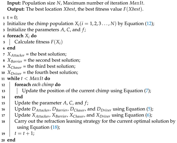
The pseudo-code of the ChOA is listed in Algorithm 1.
2.2. Principle of Light Refraction
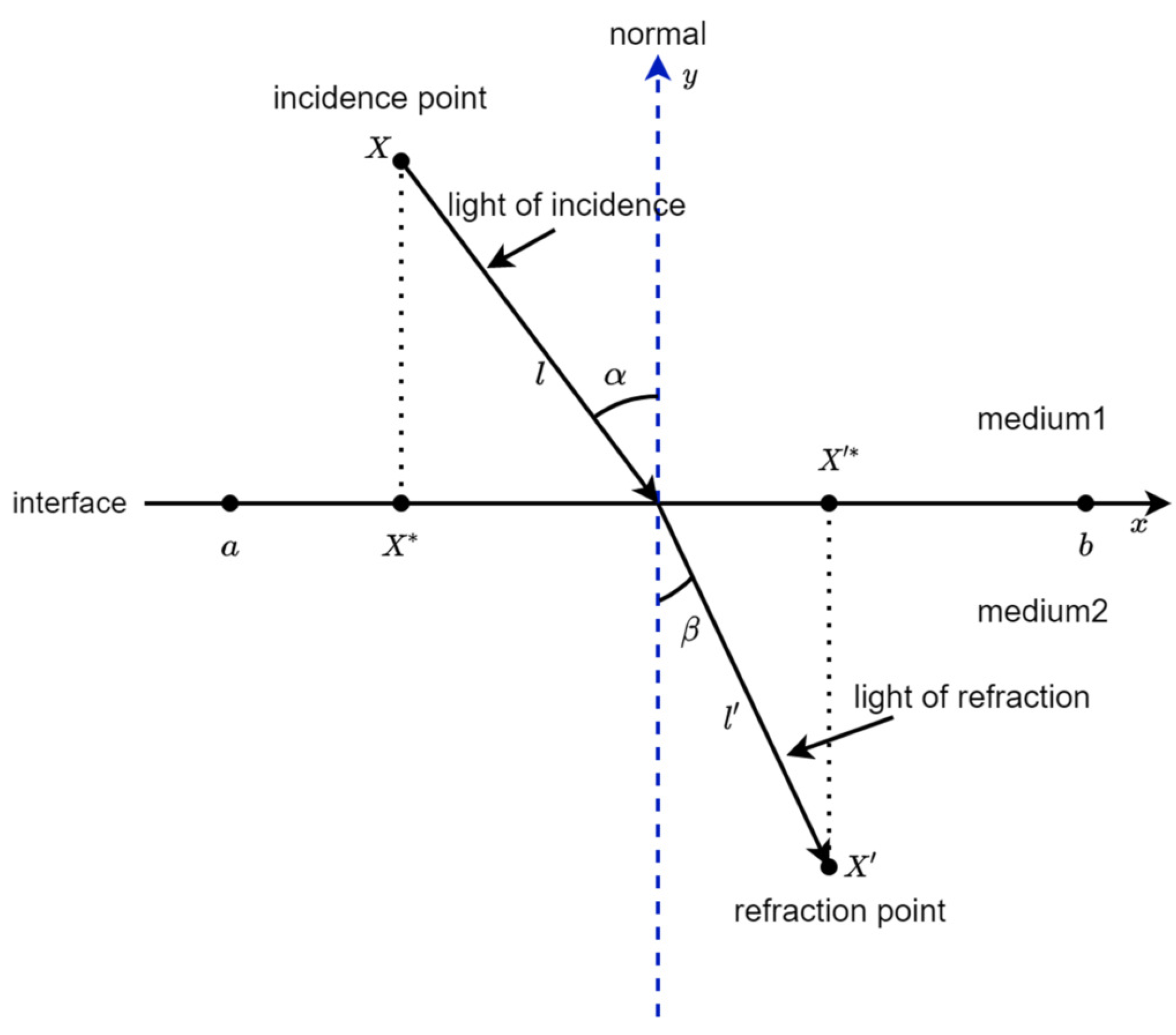
The principle of light refraction says that when light is obliquely incident from one medium into another medium, the propagation direction changes so that the speed of light changes at the junction of different media, and the deflection of the route occurs [66].
As shown in Figure 1, the light from the point P in medium 1 passes through the refraction point O, is refracted, and finally reaches the point Q in medium 2. Suppose the refractive indexes of light in medium 1 and medium 2 are and , respectively; the angle of incidence and refraction are and , respectively; and the velocities of light in medium 1 and medium 2 are and . The ratio of the sine of the angle of incidence to the angle of refraction is equal to the ratio of the reciprocals of the refraction path or the ratio of the velocities of light in two media. That is, as shown in Formula (8):
where is called the refractive index of medium 2 relative to medium 1.
| Algorithm 1: Pseudo-code of the Chimp Optimization Algorithm (ChOA). |
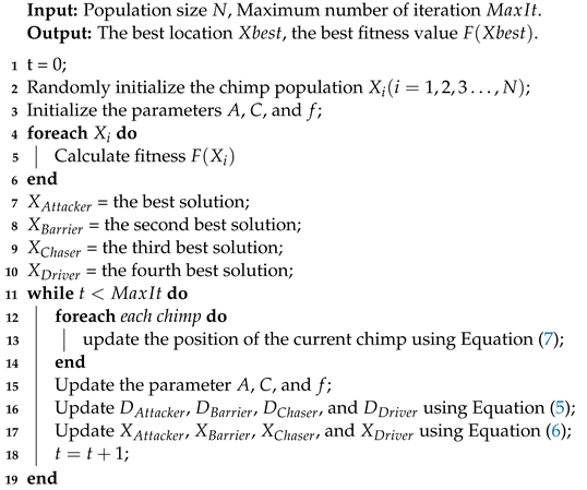 |
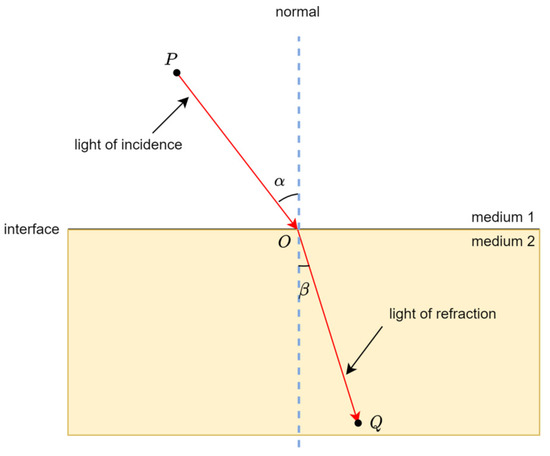
Figure 1.
Principle of light refraction.
3. Proposed RL-ChOA
3.1. Motivation
According to Equation (7), the chimp population completed the hunting process under the guidance of “Attacker”, “Barrier”, “Chaser”, and “Driver”. Mathematically, the fitter chimps (“Attacker”, “Barrier”, “Chaser”, and “Driver”) help the other chimps in the population update their positions. Therefore, the fitter chimps are mainly responsible for prey search and providing prey direction for the population. Thus, these leading chimps must have good fitness values. This way of updating the population position is conducive to attracting the population to the fitter chimps more quickly, but the diversity of the population is hindered. In the end, ChOA is trapped in a local optimum.
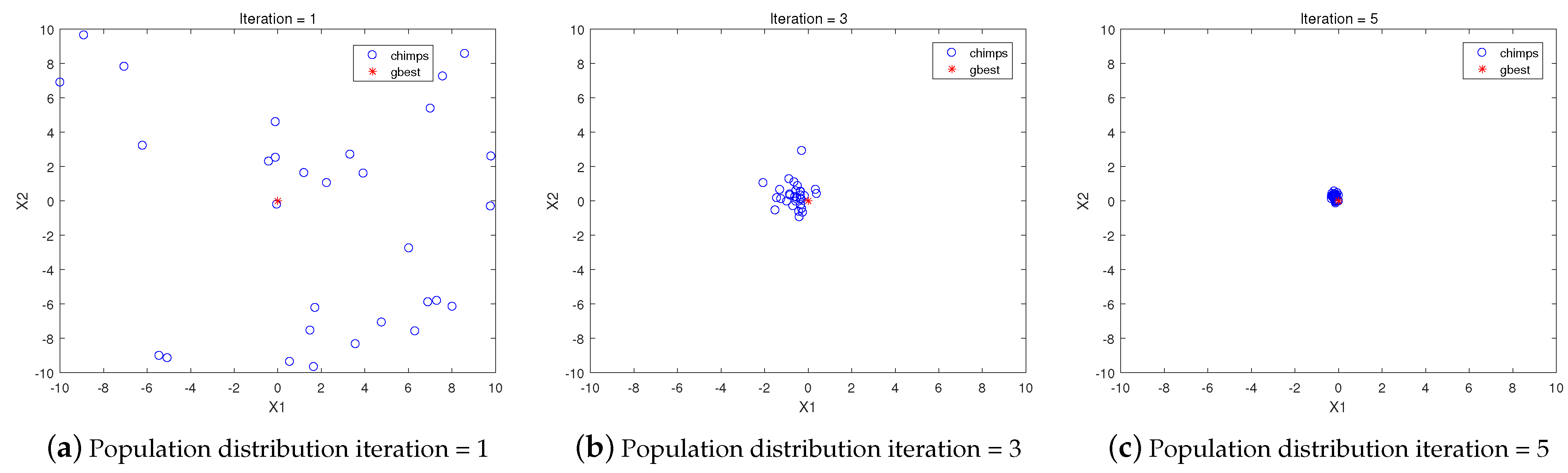
Figure 2 illustrates the 30 population distribution of the Sphere function with two dimensions in [−10, 10] observed at various stages of ChOA.
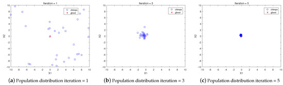
Figure 2.
Population distribution observed at various stages in RL-ChOA.
As shown in Figure 2, after initialization, the chimp population of ChOA begins to explore the entire search space. Then, led by “Attacker”, “Barrier”, “Chaser”, and “Driver”, ChOA can accumulate many chimpanzees into the optimal search space. However, due to the poor exploratory ability of other chimps in the population, if the current one is in a local optimum, then ChOA is easy to fall into a local optimum. In other words, the global exploration ability of ChOA mainly depends on the well-fitted chimps. In addition, it is noted that there is still room for further improvement in the global exploration ability of ChOA. Therefore, the population leader needs to improvise to avoid being premature due to locally optimal solutions.
3.2. Tent Chaos Sequence
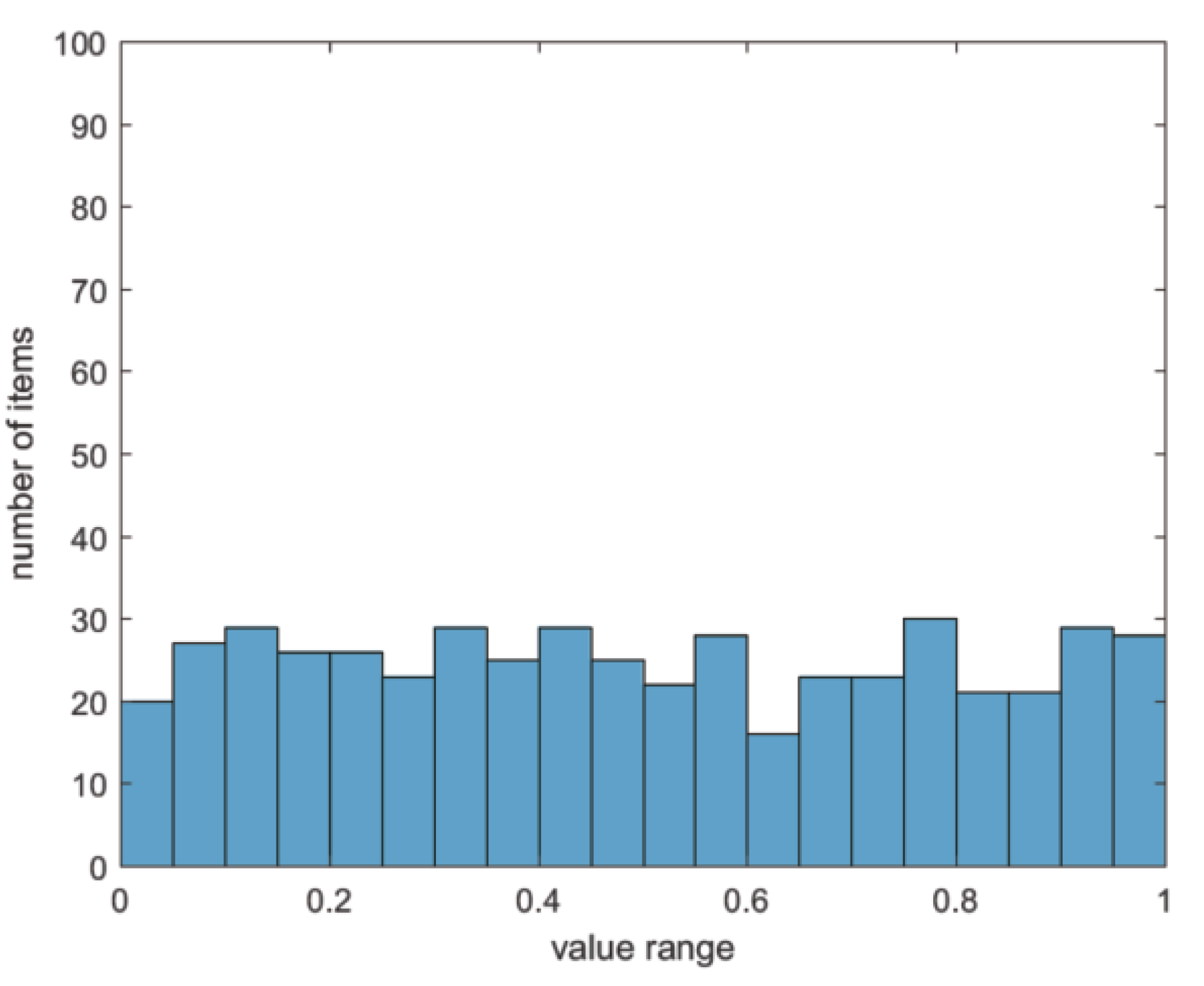
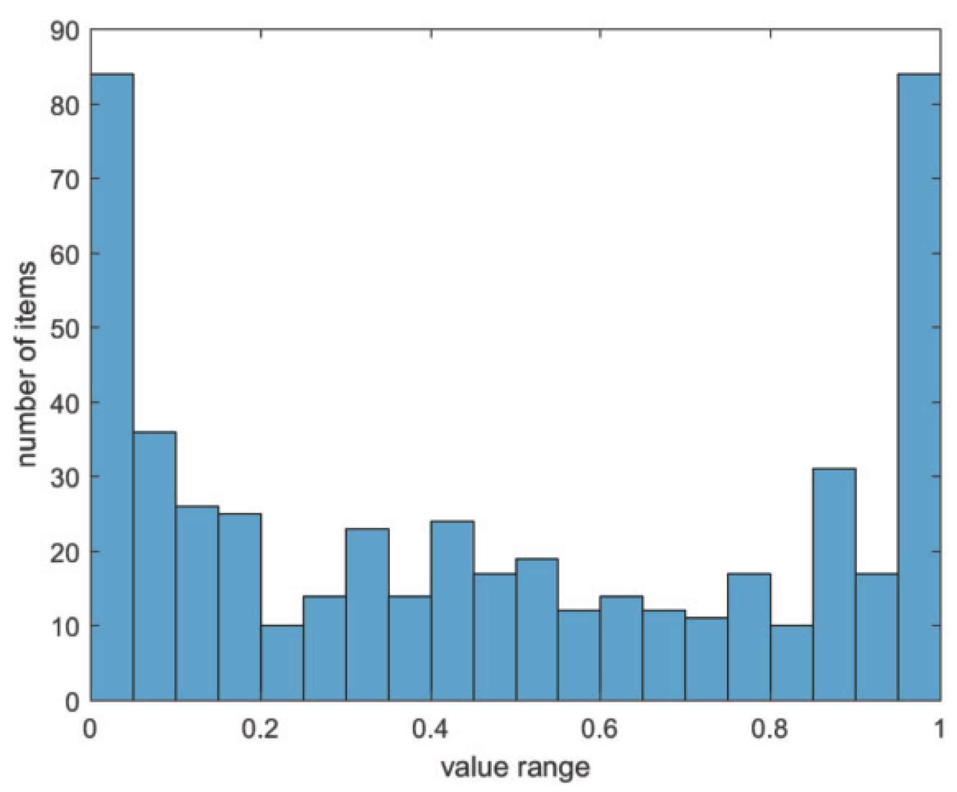
The Tent chaos sequence has the characteristics of randomness, ergodicity, and regularity [67]. Using these characteristics to optimize the search can effectively maintain the diversity of the population, suppress the algorithm from falling into the local optimum, and improve the global search ability. The original chimp optimization algorithm adopts The rand function and randomly initializes the population, and the resulting population distribution is not broad enough. This paper studies Logistic chaotic map [50] and Tent chaotic map; the results demonstrate that the Tent chaotic map has better population distribution uniformity and faster search speed than the Logistic chaotic map. Figure 3 and Figure 4 represent the histograms of the Tent chaotic sequence and the Logistics chaotic sequence, respectively. From these two figures, it can be found that the value probability of the Logistic chaotic map between and is higher than that of other segments, while the value probability of the Tent chaotic map in each segment of the feasible region is relatively uniform. Therefore, Tent chaotic map is better than the Logistic chaotic map in population initialization. In this paper, the ergodicity of the Tent chaotic map is used to generate a uniformly distributed chaotic sequence, which reduces the influence of the initial population distribution on the algorithm optimization.

Figure 3.
Tent chaotic sequence distribution histogram.

Figure 4.
Logistic chaotic sequence distribution histogram.
The expression of the Tent chaotic map is as follows:
After the Bernoulli shift transformation, the expression is as follows:
By analyzing the Tent chaotic iterative sequence, it can be found that there are short periods and unstable period points in the sequence. To avoid the Tent chaotic sequence falling into small period points and unstable period points during iteration, a random variable is introduced into the Tent chaotic map expression. Then, the improved Tent chaotic map expression is as follows:
The transformed expression is as follows:
where N is the number of particles in the sequence. is a random number in the range . The introduction of the random variable not only maintains the randomness, ergodicity, and regularity of the Tent chaotic map but can also effectively avoid iterative falling into small periodic points and unstable periodic points.
3.3. Refraction of Light Learning Strategy
Mathematically speaking, by Equations (5)–(7), in standard ChOA, the Attacker, Barrier, Chaser, and Driver are primarily responsible for searching for prey and guiding other chimps in the population to complete location updates during the hunt. However, when the Attacker, Barrier, Chaser, and Driver search for the best prey in the current local area, they will guide the entire population to gather near these four types of chimps, which will cause the algorithm to fall into local optimum and reduce population diversity. This makes the algorithm appear to be “Prematurity”.
Therefore, to solve this problem, this paper proposes a new learning strategy based on the refraction principle of light, which is used to help the population jump out of the local optimum and maintain the diversity of the population. The basic principle of refraction learning is shown in Figure 5.
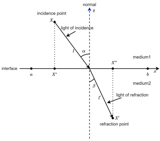
Figure 5.
One-dimensional spatial refraction learning process for the current global optima .
In Figure 5, the search space for the solution on the x-axis is ; the incident ray and the refracted ray are l and , respectively; the y-axis represents the normal; and are the angles of incidence and refraction, respectively; X and are the points of incidence and the point of reflection, respectively; the projection points of X and on the x-axis are and , respectively. From the geometric relationship of the line segments in Figure 5, the following formulas can be obtained:
From the definition of the refractive index, we know that . Combining it with the above Equations (13) and (14), the following formula can be obtained:
Let , then, the above Equation (15) can be changed into the following formula:
Convert Equation (16), and the calculation formula for the solution based on refraction learning is as follows:
When the dimension of the optimization problem is n-dimensional, and , the Equation (17) can be modified as follows:
where, and are the original value of the j-th dimension in the n-dimensional space and the value after refraction learning, respectively; and are the maximum and minimum values of the j-th dimension in the n-dimensional space, respectively. When , Equation (18) becomes as follows:
Equation (19) is a typical OBL, so it can be observed that OBL is a special kind of refraction learning.
3.4. The Framework of RL-ChOA
The framework of the proposed RL-ChOA is shown in Algorithm 2.
| Algorithm 2: Framework of the Proposed Algorithm (RL-ChOA). |
 |
3.5. Time Complexity Analysis
The time complexity [68] indirectly reflects the convergence speed of the algorithm. In the original ChOA, it is assumed that the time required for initialization of parameters (population size is N, search space dimension is n, coefficients are A, f, C, and other parameters) is ; and the time required for each individual to update its position is ; the time to solve the objective function is . Then, the time complexity of the original ChOA is as follows:
In the RL-ChOA proposed in this paper, the Tent chaos sequence is used in the population initialization, and the time spent is consistent with the original population initialization. In the algorithm loop stage, the time required to use the refraction learning strategy of light is ; and the time needed to execute the greedy mechanism is . Then, the time complexity of RL-ChOA is as follows:
The time complexity of RL-ChOA proposed in this paper is consistent with the original ChOA:
In summary, the improved strategy proposed in this paper for ChOA defects does not increase the time complexity.
3.6. Remark
In Section 3.1, the reasons why ChOA is prone to fall into local optimum and the motivation for improvement are analyzed. In Section 3.2 and Section 3.3, the strategies for improving ChOA are analyzed in detail. Based on the principle of light refraction, we propose refraction learning, and apply it to ChOA to help jump out of the local optimum and achieve a balance between a global and local search. In Section 3.4 and Section 3.5, the process framework and time complexity of RL-ChOA are analyzed.
4. Experimental Simulations
In this section, to test the optimization performance of RL-ChOA, we conducted a set of experiments using benchmark test functions. Section 4.1 describes the benchmark test suite used in the experiments, Section 4.2 describes the experimental simulation environment, and Section 4.3 describes the parameter settings.
4.1. Benchmark Test Suite
Twenty-three classical benchmark test functions, widely verified by many researchers, are used in experiments to verify the algorithm’s performance. These benchmark test functions F1–F23 can be found in [9]. Among them, F1–F7 are seven continuous unimodal benchmark test functions, and their dimensions are set to 30, which are used to test the optimization accuracy of the algorithm; F8–F13 are six continuous multi-modal benchmark test functions, and their dimensions are also set to 30, to test the algorithm’s ability to avoid prematurity; F14–F23 are nine fixed-dimension multi-modal benchmark test functions, which are used to test the global search ability and convergence speed of the algorithm. Details of the benchmark test functions, for example, the name of the function, the expression of the function, the search range of the function, and the optimal value of the function, can be found in [9].
4.2. Experimental Simulation Environment
The computer configuration used in the experimental simulation is Intel “Core i7-4720HQ”, the main frequency is “2.60 GHz”, “8 GB memory”, “Windows10 64bit” operating system and the computing environment is “Matlab2016 (a)”.
4.3. Parameter Setting
The common parameters of all algorithms are set to the same size. The population size is set to 30, the maximum fitness function call is set to 15,000, and each algorithm runs independently 30 times. The parameter settings in different algorithms are shown in Table 1.

Table 1.
Algorithm parameter setting.
5. Experimental Results
In this section, to verify the algorithm’s performance proposed in this paper, it is compared with five state-of-the-art algorithms, namely the Grey Wolf Algorithm Based on L/’evy Flight and Random Walk Strategy (MGWO) [69], improved Grey Wolf Optimization Algorithm based on iterative mapping and simplex method (SMIGWO) [70], Teaching-learning-based Optimization Algorithm with Social Psychology Theory (SPTLBO) [71], original ChOA, and WChOA. Table 2, Table 3 and Table 4 present the statistical results of the best value, average value, worst value, and standard deviation obtained by the six different algorithms on the three types of test problems. In order to accurately get statistically reasonable conclusions, Table 5, Table 6 and Table 7 use Friedman’s test [72] to rank three different types of benchmark test functions. In addition, Wilcoxon’s rank-sum test [73] is a nonparametric statistical test that can detect more complex data distributions. Table 8 shows the Wilcoxon’s rank-sum test for independent samples at the p = 0.05 level of significant difference [68]. The symbols “+”, “=”, and “−” indicate that RL-ChOA is better than, similar to, and worse than the corresponding comparison algorithms, respectively. In Section 5.2, we analyze and illustrate the convergence of RL-ChOA on 23 widely used test functions. In Section 5.3, the different values of parameters k and in the light refraction learning strategy are analyzed.
Table 2.
Results of unimodal benchmark test functions.
Table 3.
Results of multi-modal benchmark functions.
Table 4.
Results of fixed-dimension multi-modal benchmark functions.
Table 5.
Average rankings of the algorithms (Friedman) on fixed-dimension multi-modal benchmark functions.
Table 6.
Average rankings of the algorithms (Friedman) on unimodal benchmark test functions.
5.1. Experiments on 23 Widely Used Test Functions
As shown in Table 2, in the unimodal benchmark test functions (F1–F7): the overall performance of the proposed algorithm RL-ChOA is better than other algorithms on the unimodal benchmark problem. RL-ChOA can perform best compared to other algorithms except for three benchmark test functions (F5–F7) and find the optimal value in four benchmark test functions (F1–F4). The SMIGWO achieves the best performance on two benchmark test functions (F5 and F6). The WChOA obtains the best solution on the one benchmark test function (F7). In addition, KEEL software [74] was used for the Friedman rank, and the results are shown in Table 6 RL-ChOA achieved the best place.
As can be observed from Table 3, in the multi-modal benchmark test functions (F8–F13): RL-ChOA can obtain the best solution on the four benchmark test functions (F8–F11). SPTLBO can obtain the best solution on the one benchmark test function (F12). WChOA can get the best solution on the three benchmark test functions (F9, F11, and F12). SPTLBO can obtain the best solution on the one benchmark test function (F13). RL-ChOA outperforms other algorithms overall, and in Table 7, RL-ChOA ranks first in the Friedman rank.
As can be observed from Table 4, in the fixed-dimension multi-modal benchmark functions (F14–F23): SPTLBO can get the best solution on the six benchmark test functions (F14–F19). MGWO can get the best solution on the four benchmark test functions (F16–F19 and F23). SMIGWO can obtain the best solution on the five benchmark test function (F16, F17, F19, F21, and F22); RL-ChOA cannot perform well on these test functions, but RL-ChOA outperforms both original ChOA and WChOA in overall performance. As shown in Table 5, RL-ChOA ranks third in the Friedman rank.
Wilcoxon’s rank-sum test was used to verify the significant difference between RL-ChOA and the other five algorithms. The statistical results are shown in Table 8. The results prove that = 0.05, a significant difference can be observed in all cases, and RL-ChOA outperforms 12, 11, 7, 15, and 19 benchmark functions of SMIGWO, MGWO, SPTLBO, ChOA, and WChOA, respectively.
Table 7.
Average rankings of the algorithms (Friedman) on multi-modal benchmark functions.
Table 7.
Average rankings of the algorithms (Friedman) on multi-modal benchmark functions.
| Algorithm | Ranking |
|---|---|
| SMIGWO | 3.75 |
| MGWO | 3.52 |
| SPTLBO | 2.75 |
| ChOA | 4.96 |
| WChOA | 3.46 |
| RL-ChOA | 2.56 |
Table 8.
Test statistical results of Wilcoxon’s rank-sum test.
Table 8.
Test statistical results of Wilcoxon’s rank-sum test.
| Benchmark | RL-ChOA vs. SMIGWO | RL-ChOA vs. MGWO | RL-ChOA vs. SPTLBO | RL-ChOA vs. ChOA | RL-ChOA vs. WChOA | ||||||||||
|---|---|---|---|---|---|---|---|---|---|---|---|---|---|---|---|
| H | p-Value | Winner | H | p-Value | Winner | H | p-Value | Winner | H | p-Value | Winner | H | p-Value | Winner | |
| F1 | 1 | 1.21 | + | 1 | 1.21 | + | 1 | 1.21 | + | 1 | 1.21 | + | 1 | 1.21 | + |
| F2 | 1 | 1.21 | + | 1 | 1.21 | + | 1 | 1.21 | + | 1 | 1.21 | + | 1 | 1.21 | + |
| F3 | 1 | 1.21 | + | 1 | 1.21 | + | 1 | 1.21 | + | 1 | 1.21 | + | 1 | 1.21 | + |
| F4 | 1 | 1.21 | + | 1 | 1.21 | + | 1 | 1.21 | + | 1 | 1.21 | + | 1 | 1.21 | + |
| F5 | 1 | 5.49 | - | 1 | 1.17 | - | 1 | 1.78 | - | 1 | 1.78 | - | 1 | 2.99 | + |
| F6 | 1 | 3.02 | - | 1 | 1.33 | - | 1 | 4.50 | - | 1 | 1.09 | + | 1 | 2.01 | - |
| F7 | 1 | 1.87 | + | 0 | 5.79 | - | 1 | 1.04 | - | 1 | 3.51 | + | 1 | 2.37 | - |
| F8 | 1 | 3.69 | + | 0 | 2.58 | + | 1 | 2.23 | + | 0 | 3.55 | + | 1 | 3.02 | + |
| F9 | 1 | 1.20 | + | 0 | 1.61 | + | 0 | NaN | = | 1 | 1.21 | + | 0 | NaN | = |
| F10 | 1 | 1.21 | + | 1 | 3.17 | + | 1 | 8.99 | + | 1 | 1.21 | + | 1 | 1.17 | + |
| F11 | 1 | 5.58 | + | 0 | 3.34 | + | 0 | NaN | = | 1 | 1.21 | + | 0 | 3.34 | + |
| F12 | 1 | 3.69 | - | 1 | 1.69 | - | 1 | 3.02 | - | 1 | 2.87 | + | 1 | 6.28 | + |
| F13 | 1 | 3.02 | - | 1 | 3.02 | - | 1 | 3.02 | - | 1 | 5.57 | - | 1 | 2.79 | + |
| F14 | 1 | 1.02 | + | 1 | 7.29 | + | 1 | 4.31 | + | 0 | 8.19 | = | 1 | 3.20 | + |
| F15 | 1 | 3.02 | - | 1 | 1.11 | + | 1 | 3.02 | - | 0 | 7.17 | - | 1 | 8.89 | + |
| F16 | 1 | 3.02 | = | 1 | 4.08 | = | 1 | 1.99 | = | 0 | 6.31 | = | 1 | 3.02 | + |
| F17 | 1 | 5.49 | = | 1 | 2.87 | = | 1 | 1.21 | = | 0 | 2.58 | = | 1 | 3.02 | + |
| F18 | 1 | 1.17 | + | 1 | 4.44 | = | 1 | 2.78 | = | 0 | 5.40 | = | 1 | 3.85 | = |
| F19 | 1 | 2.37 | = | 1 | 2.03 | = | 1 | 1.22 | = | 0 | 9.94 | = | 1 | 3.02 | + |
| F20 | 1 | 7.96 | + | 0 | 6.63 | + | 1 | 9.79 | - | 1 | 1.17 | + | 1 | 3.02 | + |
| F21 | 1 | 7.12 | - | 1 | 8.35 | - | 1 | 3.02 | - | 0 | 7.96 | + | 1 | 7.39 | + |
| F22 | 1 | 3.02 | - | 1 | 3.02 | - | 1 | 3.02 | - | 1 | 1.78 | + | 1 | 3.02 | + |
| F23 | 1 | 3.02 | - | 1 | 3.02 | - | 1 | 3.02 | - | 0 | 3.11 | + | 1 | 3.02 | + |
| +/−/= | 12/8/3 | 11/8/4 | 7/10/6 | 15/3/5 | 19/2/2 | ||||||||||
5.2. Convergence Analysis
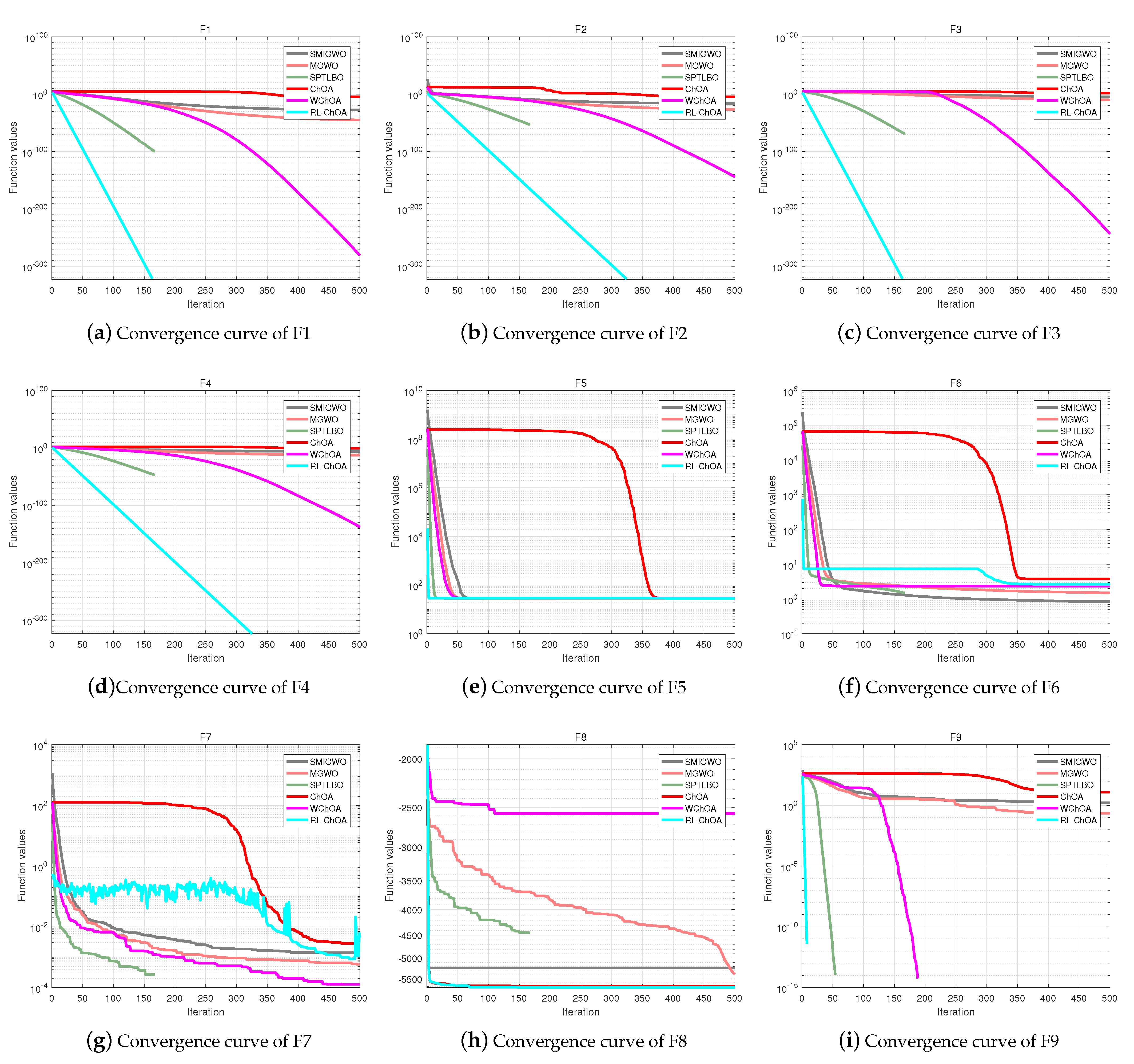
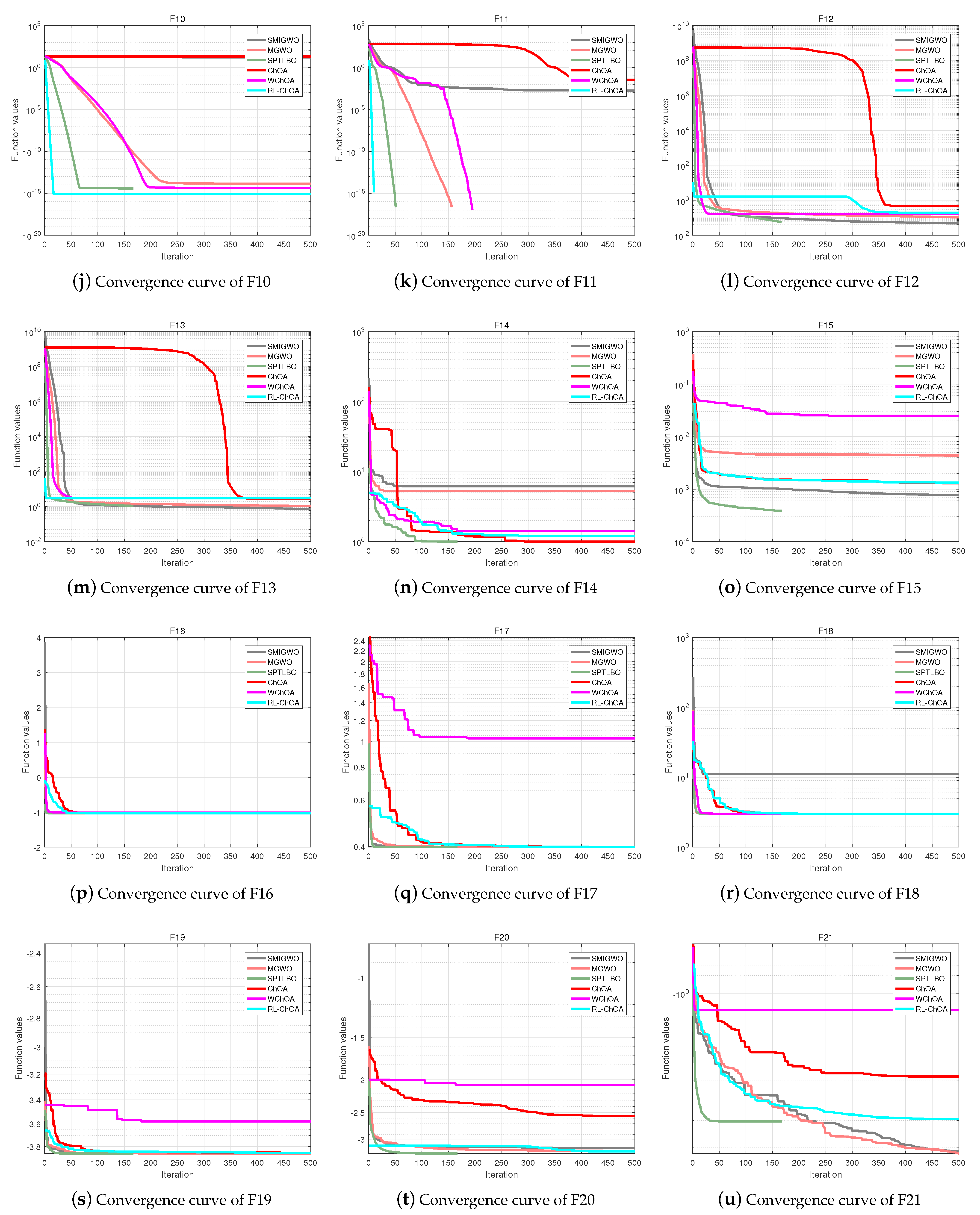
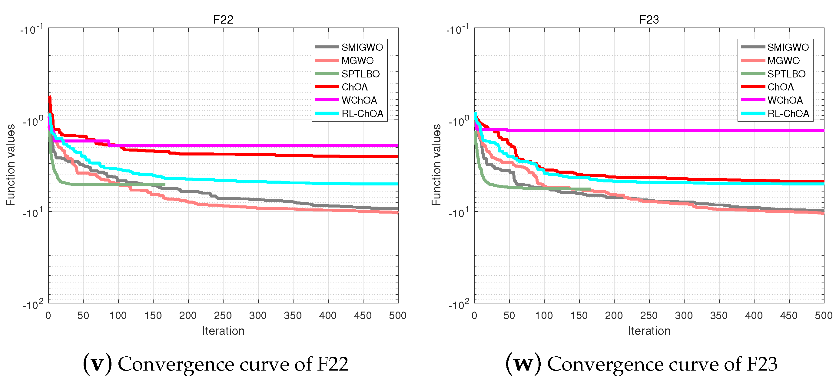
To analyze the convergence of the proposed RL-ChOA, Figure 6 shows the convergence curves of SMIGWO, MGWO, SPTLBO, ChOA, WChOA, and RL-ChOA with the increasing number of iterations. In Figure 6, the x-axis represents the number of algorithm iterations, and the y-axis represents the optimal value of the function. It can be observed that the convergence speed of RL-ChOA is significantly better than that of other algorithms because the learning strategy, based on light refraction, can enable the optimal individual to find a better position in the solution space and lead other individuals to approach this position quickly. RL-ChOA has apparent advantages in unimodal benchmark functions and multi-modal benchmark functions. However, despite poor performance on the fixed-dimensional multi-modal benchmark function RL-ChOA, it outperforms the original ChOA and the improved ChOA-based WChOA. RL-ChOA is sufficiently competitive with other state-of-the-art heuristic algorithms in terms of overall performance.
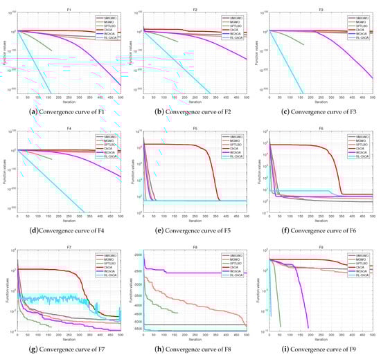
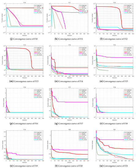

Figure 6.
Convergence figures on test functions F1–F23.
5.3. Parameter Sensitivity Analysis
The refraction learning of light as described in Section 3.3, and the parameters and k in Equation (18), are the keys to improving the performance of RL-ChOA. In this subsection, to investigate the sensitivity of parameters and k, a series of experiments are conducted, and it is concluded that RL-ChOA performs best when the values of parameters and k are in . We tested RL-ChOA with different : 1, 10, 100 and 1000, and different k: 1, 10, 100 and 1000. The benchmark functions are the same as those selected in Section 4.1. The parameter settings are the same as in Section 4.3. Table 5 summarizes the mean and standard deviation of the test function values for RL-ChOA using different and k combinations. As shown in Table 9, when parameters and k are set to 100 and 100, respectively, RL-ChOA outperforms other parameter settings in most test functions.
5.4. Remarks
According to the above results: (1) RL-ChOA has excellent performance on the unimodal benchmark test functions and the multi-modal benchmark test function because the best individual uses the light refraction-based learning strategy to improve the algorithm’s global exploration ability. In addition, Tent chaos sequence was introduced to increase the diversity of the population and improve search accuracy and convergence speed. However, the performance needs to improve on fixed-dimension multi-modal benchmark functions. (2) RL-ChOA outperforms the original ChOA and the improved WChOA based on ChOA, whether on the multi-modal benchmark test functions, the unimodal benchmark test functions, or the fixed-dimension multi-modal benchmark functions.
Table 9.
Experimental results of RL-ChOA using different combinations of k and .
Table 9.
Experimental results of RL-ChOA using different combinations of k and .
| Function | = 1, k = 1 | = 10, k = 10 | = 100, k = 100 | = 1000, k = 1000 | ||||
|---|---|---|---|---|---|---|---|---|
| Mean | St.dev | Mean | St.dev | Mean | St.dev | Mean | St.dev | |
| F1 | 2.9363 | 9.7403 | 0.0000 | 0.0000 | 0.0000 | 0.0000 | 0.0000 | 0.0000 |
| F2 | 3.6343 | 4.0394 | 0.0000 | 0.0000 | 0.0000 | 0.0000 | 0.0000 | 0.0000 |
| F3 | 1.0063 | 5.4903 | 0.0000 | 0.0000 | 0.0000 | 0.0000 | 0.0000 | 0.0000 |
| F4 | 3.1650 | 7.3138 | 0.0000 | 0.0000 | 0.0000 | 0.0000 | 0.0000 | 0.0000 |
| F5 | 2.8968 | 6.6944 | 2.8975 | 5.5369 | 2.8732 | 3.0079 | 2.8974 | 5.6955 |
| F6 | 4.9292 | 3.0194 | 4.2253 | 6.1582 | 4.1277 | 5.4895 | 4.2277 | 7.4070 |
| F7 | 2.6141 | 2.0053 | 4.1955 | 1.2170 | 2.5403 | 2.5588 | 3.5305 | 3.8636 |
| F8 | −6.1749 | 3.5394 | −6.0819 | 3.4058 | −6.2563 | 4.2758 | −6.1964 | 4.3861 |
| F9 | 0.0000 | 0.0000 | 0.0000 | 0.0000 | 0.0000 | 0.0000 | 0.0000 | 0.0000 |
| F10 | 1.2375 | 4.7283 | 8.8818 | 0.0000 | 8.8818 | 0.0000 | 8.8818 | 0.0000 |
| F11 | 9.1245 | 2.8466 | 0.0000 | 0.0000 | 0.0000 | 0.0000 | 0.0000 | 0.0000 |
| F12 | 7.1215 | 2.2662 | 6.1241 | 1.5222 | 5.9170 | 1.5623 | 6.1394 | 1.8421 |
| F13 | 2.7715 | 9.6490 | 2.9987 | 4.0780 | 2.9988 | 3.1025 | 2.9989 | 4.7321 |
| F14 | 1.2980 | 6.0103 | 1.0710 | 2.5954 | 1.0123 | 5.8488 | 1.2268 | 5.5093 |
| F15 | 1.3967 | 8.3618 | 1.3964 | 9.0421 | 1.3763 | 7.3362 | 1.4112 | 7.8338 |
| F16 | −1.0316 | 4.0525 | −1.0316 | 2.1053 | −1.0316 | 3.7042 | −1.0316 | 2.9538 |
| F17 | 3.9821 | 3.8502 | 3.9820 | 4.5274 | 3.9822 | 2.9042 | 3.9816 | 2.7264 |
| F18 | 3.0002 | 2.7370 | 3.0003 | 3.9395 | 3.0002 | 3.5075 | 3.0003 | 4.1256 |
| F19 | −3.8555 | 2.2133 | −3.8551 | 2.0785 | −3.8551 | 1.9819 | −3.8553 | 2.0139 |
| F20 | −3.2830 | 1.9182 | −3.2941 | 1.4701 | −3.2940 | 1.5499 | −3.2893 | 1.7582 |
| F21 | −2.9032 | 2.0892 | −3.6353 | 1.9805 | −4.2423 | 1.5862 | −3.3565 | 2.0556 |
| F22 | −2.1130 | 1.9578 | −4.3551 | 1.5668 | −4.4875 | 1.4273 | −4.0791 | 1.7789 |
| F23 | −5.0784 | 2.5185 | −4.9409 | 7.5430 | −5.0880 | 1.9410 | −4.9393 | 7.5488 |
6. RL-ChOA Engineering Example Application Analysis
This section aims further to explore the excellent performance of RL-ChOA in practical engineering. Welded beam engineering [59] is discussed in Section 6.1, tension/compression spring optimal design [59] is addressed in summary Section 6.2, and the results are compared with PSO, GA, ChOA, and WChOA.
6.1. Welded Beam Design Problem
The structure of the welded beam [59] is shown in Figure 7. The goal of structural design optimization of welded beams is to minimize the total cost under certain constraints. The design variables are: , , and , and the constraints are the shear stress , the bending stress on the beam, the buckling critical load and the tail of the beam, and beam deflection . The objective function and constraints are as follows:
Figure 7.
Design principle of the welded beam.
Consider:
Subject to:
where
with
Table 10 shows the average value of each optimization result of the five algorithms for solving the welded beam design problem. Each algorithm is independently run 50 times, the maximum number of iterations is 1000, and the population size is 30.
Table 10.
Comparison of welded beam design.
It can be observed from Table 10 that RL-ChOA shows superior performance on the optimization problem of welded beams. Although the single variable is not optimal, it is optimal in terms of the total cost.
6.2. Extension/Compression Spring Optimization Design Problem
The optimization goal of the extension/compression spring design problem [59] is to reduce the weight of the spring, the schematic diagram of which is shown in Figure 8. Constraints include subject to minimum deviation (), shear stress (), shock frequency (), outer diameter limit (), and decision variables include wire diameter d, average coil diameter D, and effective coil number P, to minimize spring weight. The objective functions and constraints of these three optimization variables are as follows:
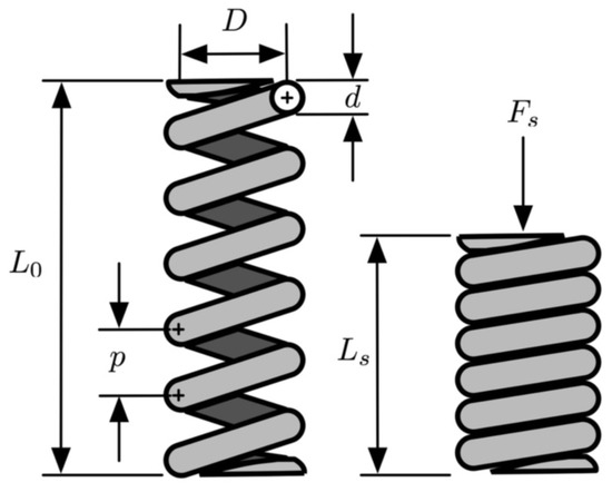
Figure 8.
Extension/compression spring structure.
Table 11 shows the average value of each optimization result of the five algorithms for solving the extension/compression spring design optimization problem. Each algorithm is independently run 50 times, the maximum number of iterations is 1000, and the population size is 30.
Table 11.
Comparison of tension/compression spring design.
It can be observed from Table 11 that RL-ChOA shows superior performance on the optimization problem of welded beams.
7. Conclusions
This paper proposes an improved ChOA based on the learning strategy of light reflection (RL-ChOA) based on the original ChOA. An improved Tent chaos sequence was introduced to increase the diversity of the population and improve search accuracy and convergence speed. In addition, a new refraction learning strategy is proposed and introduced into the original ChOA based on the principle of physical light refraction to help the population jump out of the local optimum. First, it uses 23 widely used benchmark functions and Wilcoxon’s rank-sum test verify that RL-ChOA has better optimization performance and stronger robustness. Our source code is available on https://github.com/zhangquan123-zq/RL-ChOA (accessed on 20 April 2022).
In the future, some work needs to be conducted to further improve the algorithm’s performance. An adaptive parameter strategy is designed to improve the optimization performance of RL-ChOA. The optimization effectiveness of RL-ChOA is tested on some difficult benchmark functions [75,76,77]. Some more multi-dimensional engineering problems are used to verify the engineering validity of RL-ChOA.
Author Contributions
Conceptualization, S.D.; Data curation, K.D. and H.W.; formal analysis, Y.L. and K.D.; investigation, S.D. and Y.L.; Funding acquisition, S.D.; Supervision, S.D.; resources, Q.Z., S.D. and Y.Z.; software, Q.Z.; writing—original draft preparation, Q.Z. and S.D.; writing—review and editing, S.D. and Y.Z.; visualisation, H.W. All authors have read and agreed to the published version of the manuscript.
Funding
The present work was supported by the National Natural Science Foundation of China (Grant No. 21875271, U20B2021), the Entrepreneuship Program of Foshan National Hi-tech Industrial Development Zone and Zhejiang Province Key Research and Development Program (No. 2019C01060), “Pioneer” and “Leading Goose” R&D Program of Zhejiang (Grant No. 2022C01236), International Partnership Program of Chinese Academy of Sciences (Grant No. 174433KYSB20190019), and Leading Innovative and Entrepreneur Team Introduction Program of Zhejiang (Grant No. 2019R01003).
Institutional Review Board Statement
Not applicable.
Informed Consent Statement
Not applicable.
Data Availability Statement
Not applicable.
Conflicts of Interest
The authors declare no conflict of interest.
References
- Goldberg, D.E. Genetic Algorithms in Search, Optimization and Machine Learning, 1st ed.; Addison-Wesley Longman Publishing Co., Inc.: Boston, MA, USA, 1989. [Google Scholar]
- Van Laarhoven, P.J.M.; Aarts, E.H.L. Simulated annealing. In Simulated Annealing: Theory and Applications; Springer: Dordrecht, The Netherlands, 1987; pp. 7–15. [Google Scholar] [CrossRef]
- Hussien, A.G.; Amin, M.; Wang, M.; Liang, G.; Alsanad, A.; Gumaei, A.; Chen, H. Crow search algorithm: Theory, recent advances, and applications. IEEE Access 2020, 8, 173548–173565. [Google Scholar] [CrossRef]
- Dorigo, M.; Birattari, M.; Stutzle, T. Ant colony optimization. IEEE. Comput. Intell. Mag. 2006, 1, 28–39. [Google Scholar] [CrossRef]
- Storn, R.; Price, K. Differential Evolution—A Simple and Efficient Heuristic for global Optimization over Continuous Spaces. J. Glob. Optim. 1997, 11, 341–359. [Google Scholar] [CrossRef]
- Kennedy, J.; Eberhart, R. Particle swarm optimization. In Proceedings of the ICNN’95-International Conference on Neural Networks, Perth, Australia, 27 November–1 December 1995; IEEE: Piscataway, NJ, USA, 1995; Volume 4, pp. 1942–1948. [Google Scholar]
- Yang, X.S. A New Metaheuristic Bat-Inspired Algorithm. In Nature Inspired Cooperative Strategies for Optimization (NICSO 2010); Springer: Berlin/Heidelberg, Germany, 2010; pp. 65–74. [Google Scholar] [CrossRef] [Green Version]
- Gandomi, A.H.; Yang, X.S.; Alavi, A.H. Cuckoo search algorithm: A metaheuristic approach to solve structural optimization problems. Eng. Comput. 2013, 29, 17–35. [Google Scholar] [CrossRef]
- Mirjalili, S.; Lewis, A. The Whale Optimization Algorithm. Adv. Eng. Softw. 2016, 95, 51–67. [Google Scholar] [CrossRef]
- Yang, X.S. Firefly Algorithms for Multimodal Optimization. In Proceedings of the Stochastic Algorithms: Foundations and Applications, Sapporo, Japan, 26–28 October 2009; Watanabe, O., Zeugmann, T., Eds.; Springer: Berlin/Heidelberg, Germany, 2009; pp. 169–178. [Google Scholar]
- Mirjalili, S.; Mirjalili, S.M.; Lewis, A. Grey Wolf Optimizer. Adv. Eng. Softw. 2014, 69, 46–61. [Google Scholar] [CrossRef] [Green Version]
- Rao, R.; Savsani, V.; Vakharia, D. Teaching–Learning-Based Optimization: An optimization method for continuous non-linear large scale problems. Inf. Sci. 2012, 183, 1–15. [Google Scholar] [CrossRef]
- Karaboga, D.; Basturk, B. A powerful and efficient algorithm for numerical function optimization: Artificial bee colony (ABC) algorithm. J. Glob. Optim. 2007, 39, 459–471. [Google Scholar] [CrossRef]
- Khishe, M.; Mosavi, M. Chimp optimization algorithm. Expert Syst. Appl. 2020, 149, 113338. [Google Scholar] [CrossRef]
- Masehian, E.; Sedighizadeh, D. A multi-objective PSO-based algorithm for robot path planning. In Proceedings of the 2010 IEEE International Conference on Industrial Technology, Viña del Mar, Chile, 14–17 March 2010; pp. 465–470. [Google Scholar] [CrossRef]
- Zhang, Y.; Wang, J.; Li, X.; Huang, S.; Wang, X. Feature Selection for High-Dimensional Datasets through a Novel Artificial Bee Colony Framework. Algorithms 2021, 14, 324. [Google Scholar] [CrossRef]
- Chuang, L.Y.; Chang, H.W.; Tu, C.J.; Yang, C.H. Improved binary PSO for feature selection using gene expression data. Comput. Biol. Chem. 2008, 32, 29–38. [Google Scholar] [CrossRef] [PubMed]
- Almomani, O. A Feature Selection Model for Network Intrusion Detection System Based on PSO, GWO, FFA and GA Algorithms. Symmetry 2020, 12, 1046. [Google Scholar] [CrossRef]
- Li, X.; Xiao, S.; Wang, C.; Yi, J. Mathematical modeling and a discrete artificial bee colony algorithm for the welding shop scheduling problem. Memet. Comput. 2019, 11, 371–389. [Google Scholar] [CrossRef]
- Jayabarathi, T.; Raghunathan, T.; Adarsh, B.; Suganthan, P.N. Economic dispatch using hybrid grey wolf optimizer. Energy 2016, 111, 630–641. [Google Scholar] [CrossRef]
- Emary, E.; Zawbaa, H.M.; Grosan, C. Experienced Gray Wolf Optimization Through Reinforcement Learning and Neural Networks. IEEE Trans. Neural Netw. Learn. Syst. 2018, 29, 681–694. [Google Scholar] [CrossRef]
- Yu, J.; Liu, G.; Xu, J.; Zhao, Z.; Chen, Z.; Yang, M.; Wang, X.; Bai, Y. A Hybrid Multi-Target Path Planning Algorithm for Unmanned Cruise Ship in an Unknown Obstacle Environment. Sensors 2022, 22, 2429. [Google Scholar] [CrossRef]
- Al-Shourbaji, I.; Helian, N.; Sun, Y.; Alshathri, S.; Abd Elaziz, M. Boosting Ant Colony Optimization with Reptile Search Algorithm for Churn Prediction. Mathematics 2022, 10, 1031. [Google Scholar] [CrossRef]
- Khairuzzaman, A.K.M.; Chaudhury, S. Multilevel thresholding using grey wolf optimizer for image segmentation. Expert Syst. Appl. 2017, 86, 64–76. [Google Scholar] [CrossRef]
- Papakostas, G.A.; Nolan, J.W.; Mitropoulos, A.C. Nature-Inspired Optimization Algorithms for the 3D Reconstruction of Porous Media. Algorithms 2020, 13, 65. [Google Scholar] [CrossRef] [Green Version]
- Wang, M.; Chen, H.; Li, H.; Cai, Z.; Zhao, X.; Tong, C.; Li, J.; Xu, X. Grey wolf optimization evolving kernel extreme learning machine: Application to bankruptcy prediction. Eng. Appl. Artif. Intell. 2017, 63, 54–68. [Google Scholar] [CrossRef]
- Precup, R.E.; David, R.C.; Petriu, E.M. Grey Wolf Optimizer Algorithm-Based Tuning of Fuzzy Control Systems with Reduced Parametric Sensitivity. IEEE Trans. Ind. Electron. 2017, 64, 527–534. [Google Scholar] [CrossRef]
- Marinaki, M.; Marinakis, Y.; Stavroulakis, G.E. Fuzzy control optimized by PSO for vibration suppression of beams. Control. Eng. Pract. 2010, 18, 618–629. [Google Scholar] [CrossRef]
- Fierro, R.; Castillo, O. Design of Fuzzy Control Systems with Different PSO Variants. In Recent Advances on Hybrid Intelligent Systems; Castillo, O., Melin, P., Kacprzyk, J., Eds.; Springer: Berlin/Heidelberg, Germany, 2013; pp. 81–88. [Google Scholar] [CrossRef]
- Dasu, B.; Sivakumar, M.; Srinivasarao, R. Interconnected multi-machine power system stabilizer design using whale optimization algorithm. Prot. Control. Mod. Power Syst. 2019, 4, 2. [Google Scholar] [CrossRef]
- Del Valle, Y.; Venayagamoorthy, G.K.; Mohagheghi, S.; Hernandez, J.C.; Harley, R.G. Particle Swarm Optimization: Basic Concepts, Variants and Applications in Power Systems. IEEE Trans. Evol. 2008, 12, 171–195. [Google Scholar] [CrossRef]
- AlRashidi, M.R.; El-Hawary, M.E. A Survey of Particle Swarm Optimization Applications in Electric Power Systems. IEEE Trans. Evol. 2009, 13, 913–918. [Google Scholar] [CrossRef]
- Panwar, L.K.; Reddy K, S.; Verma, A.; Panigrahi, B.; Kumar, R. Binary Grey Wolf Optimizer for large scale unit commitment problem. Swarm Evol. Comput. 2018, 38, 251–266. [Google Scholar] [CrossRef]
- Jebaraj, L.; Venkatesan, C.; Soubache, I.; Rajan, C.C.A. Application of differential evolution algorithm in static and dynamic economic or emission dispatch problem: A review. Renew. Sustain. Energy Rev. 2017, 77, 1206–1220. [Google Scholar] [CrossRef]
- Couceiro, M.S.; Rocha, R.P.; Ferreira, N.M.F. A novel multi-robot exploration approach based on Particle Swarm Optimization algorithms. In Proceedings of the 2011 IEEE International Symposium on Safety, Security, and Rescue Robotics, Kyoto, Japan, 1–5 November 2011; pp. 327–332. [Google Scholar] [CrossRef]
- Ghanem, W.A.H.M.; Jantan, A. A Cognitively Inspired Hybridization of Artificial Bee Colony and Dragonfly Algorithms for Training Multi-layer Perceptrons. Cognit. Comput. 2018, 10, 1096–1134. [Google Scholar] [CrossRef]
- Oliva, D.; Abd El Aziz, M.; Ella Hassanien, A. Parameter estimation of photovoltaic cells using an improved chaotic whale optimization algorithm. Appl. Energy 2017, 200, 141–154. [Google Scholar] [CrossRef]
- Pham, Q.V.; Mirjalili, S.; Kumar, N.; Alazab, M.; Hwang, W.J. Whale Optimization Algorithm with Applications to Resource Allocation in Wireless Networks. IEEE Trans. Veh. Technol. 2020, 69, 4285–4297. [Google Scholar] [CrossRef]
- Mittal, N.; Singh, U.; Sohi, B.S. Modified grey wolf optimizer for global engineering optimization. Appl. Comput. Intell. Soft Comput. 2016, 2016, 7950348. [Google Scholar] [CrossRef] [Green Version]
- Rodríguez, L.; Castillo, O.; Soria, J. Grey wolf optimizer with dynamic adaptation of parameters using fuzzy logic. In Proceedings of the 2016 IEEE Congress on Evolutionary Computation (CEC), Vancouver, BC, Canada, 24–29 July 2016; pp. 3116–3123. [Google Scholar] [CrossRef]
- Luo, Q.; Zhang, S.; Li, Z.; Zhou, Y. A Novel Complex-Valued Encoding Grey Wolf Optimization Algorithm. Algorithms 2016, 9, 4. [Google Scholar] [CrossRef]
- Wang, H.; Liao, L.; Wang, D.; Wen, S.; Deng, M. Improved artificial bee colony algorithm and its application in LQR controller optimization. Math. Probl. Eng. 2014, 2014, 695637. [Google Scholar] [CrossRef]
- Shi, Y.; Pun, C.M.; Hu, H.; Gao, H. An improved artificial bee colony and its application. Knowl. Based Syst. 2016, 107, 14–31. [Google Scholar] [CrossRef]
- Mostafa Bozorgi, S.; Yazdani, S. IWOA: An improved whale optimization algorithm for optimization problems. Mostafa Bozorgi 2019, 6, 243–259. [Google Scholar] [CrossRef]
- Chaudhuri, A.; Sahu, T.P. Feature selection using Binary Crow Search Algorithm with time varying flight length. Expert Syst. Appl. 2021, 168, 114288. [Google Scholar] [CrossRef]
- Chen, M.R.; Huang, Y.Y.; Zeng, G.Q.; Lu, K.D.; Yang, L.Q. An improved bat algorithm hybridized with extremal optimization and Boltzmann selection. Expert Syst. Appl. 2021, 175, 114812. [Google Scholar] [CrossRef]
- Hassan, B.A. CSCF: A chaotic sine cosine firefly algorithm for practical application problems. Neural. Comput. Appl. 2021, 33, 7011–7030. [Google Scholar] [CrossRef]
- Rahnamayan, S.; Tizhoosh, H.R.; Salama, M.M.A. Opposition-Based Differential Evolution. IEEE Trans. Evol. Comput. 2008, 12, 64–79. [Google Scholar] [CrossRef] [Green Version]
- Xu, Q.; Wang, L.; Wang, N.; Hei, X.; Zhao, L. A review of opposition-based learning from 2005 to 2012. Eng. Appl. Artif. Intell. 2014, 29, 1–12. [Google Scholar] [CrossRef]
- Demir, F.B.; Tuncer, T.; Kocamaz, A.F. A chaotic optimization method based on logistic-sine map for numerical function optimization. Neural Comput. Appl. 2020, 32, 14227–14239. [Google Scholar] [CrossRef]
- Ling, Y.; Zhou, Y.; Luo, Q. Lévy flight trajectory-based whale optimization algorithm for global optimization. IEEE Access 2017, 5, 6168–6186. [Google Scholar] [CrossRef]
- Wang, H.; Wu, Z.; Rahnamayan, S.; Liu, Y.; Ventresca, M. Enhancing particle swarm optimization using generalized opposition-based learning. Inf. Sci. 2011, 181, 4699–4714. [Google Scholar] [CrossRef]
- Ewees, A.A.; Abd Elaziz, M.; Houssein, E.H. Improved grasshopper optimization algorithm using opposition-based learning. Expert Syst. Appl. 2018, 112, 156–172. [Google Scholar] [CrossRef]
- Liu, Y.; Cao, B. A Novel Ant Colony Optimization Algorithm with Levy Flight. IEEE Access 2020, 8, 67205–67213. [Google Scholar] [CrossRef]
- Kuang, F.; Jin, Z.; Xu, W.; Zhang, S. A novel chaotic artificial bee colony algorithm based on Tent map. In Proceedings of the 2014 IEEE Congress on Evolutionary Computation (CEC), Beijing, China, 6–11 July 2014; pp. 235–241. [Google Scholar] [CrossRef]
- Suresh, S.; Lal, S.; Reddy, C.S.; Kiran, M.S. A Novel Adaptive Cuckoo Search Algorithm for Contrast Enhancement of Satellite Images. IEEE J. Sel. Top. Appl. Earth Obs. Remote Sens. 2017, 10, 3665–3676. [Google Scholar] [CrossRef]
- Afrabandpey, H.; Ghaffari, M.; Mirzaei, A.; Safayani, M. A novel Bat Algorithm based on chaos for optimization tasks. In Proceedings of the 2014 Iranian Conference on Intelligent Systems (ICIS), Bam, Iran, 4–6 February 2014; pp. 1–6. [Google Scholar] [CrossRef]
- Khishe, M.; Nezhadshahbodaghi, M.; Mosavi, M.R.; Martín, D. A Weighted Chimp Optimization Algorithm. IEEE Access 2021, 9, 158508–158539. [Google Scholar] [CrossRef]
- Kaur, M.; Kaur, R.; Singh, N.; Dhiman, G. SChoA: A newly fusion of sine and cosine with chimp optimization algorithm for HLS of datapaths in digital filters and engineering applications. Eng. Comput. 2021, 1–29. [Google Scholar] [CrossRef]
- Jia, H.; Sun, K.; Mosavi; Zhang, W.; Leng, X. An enhanced chimp optimization algorithm for continuous optimization domains. Complex Intell. Syst. 2022, 8, 65–82. [Google Scholar] [CrossRef]
- Houssein, E.H.; Emam, M.M.; Ali, A.A. An efficient multilevel thresholding segmentation method for thermography breast cancer imaging based on improved chimp optimization algorithm. Expert Syst. Appl. 2021, 185, 115651. [Google Scholar] [CrossRef]
- Wang, J.; Khishe, M.; Kaveh, M.; Mohammadi, H. Binary Chimp Optimization Algorithm (BChOA): A New Binary Meta-heuristic for Solving Optimization Problems. Cognit. Comput. 2021, 13, 1297–1316. [Google Scholar] [CrossRef]
- Hu, T.; Khishe, M.; Mohammadi, M.; Parvizi, G.R.; Taher Karim, S.H.; Rashid, T.A. Real-time COVID-19 diagnosis from X-Ray images using deep CNN and extreme learning machines stabilized by chimp optimization algorithm. Biomed. Signal Process. Control 2021, 68, 102764. [Google Scholar] [CrossRef] [PubMed]
- Wu, D.; Zhang, W.; Jia, H.; Leng, X. Simultaneous Feature Selection and Support Vector Machine Optimization Using an Enhanced Chimp Optimization Algorithm. Algorithms 2021, 14, 282. [Google Scholar] [CrossRef]
- Wolpert, D.; Macready, W. No free lunch theorems for optimization. IEEE Trans. Evol. 1997, 1, 67–82. [Google Scholar] [CrossRef] [Green Version]
- Born, M.; Wolf, E. Principles of Optics: 60th Anniversary Edition, 7th ed.; Cambridge University Press: Cambridge, UK, 2019. [Google Scholar] [CrossRef]
- Liu, L.; Sun, S.Z.; Yu, H.; Yue, X.; Zhang, D. A modified Fuzzy C-Means (FCM) Clustering algorithm and its application on carbonate fluid identification. J. Appl. Geophy. 2016, 129, 28–35. [Google Scholar] [CrossRef]
- Derrac, J.; García, S.; Molina, D.; Herrera, F. A practical tutorial on the use of nonparametric statistical tests as a methodology for comparing evolutionary and swarm intelligence algorithms. Swarm Evol. Comput. 2011, 1, 3–18. [Google Scholar] [CrossRef]
- Li, Y.; Li, W.; Zhao, Y.; Liu, A. Grey Wolf Algorithm Based on Levy Flight and Random Walk Strategy. Comput. Sci. 2020, 47, 291–296. [Google Scholar]
- Wang, M.; Wang, Q.; Wang, X. Improved grey wolf optimization algorithm based on iterative mapping and simplex method. J. Comput. Appl. 2018, 38, 16–20, 54. [Google Scholar]
- He, P.; Liu, Y. Teaching-learning-based Optimization Algorithm with Social Psychology Theory. J. Front. Comput. Sci. Technol. 2021, 44, 1–16. [Google Scholar]
- Sheldon, M.R.; Fillyaw, M.J.; Thompson, W.D. The use and interpretation of the Friedman test in the analysis of ordinal-scale data in repeated measures designs. Physiother. Res. Int. 1996, 1, 221–228. [Google Scholar] [CrossRef]
- Rey, D.; Neuhäuser, M. Wilcoxon-signed-rank test. In International Encyclopedia of Statistical Science; Springer: Berlin/Heidelberg, Germany, 2011; pp. 1658–1659. [Google Scholar]
- Introduction to KEEL Software Suite. Available online: https://sci2s.ugr.es/keel/development.php (accessed on 7 April 2022).
- Garg, V.; Deep, K. Performance of Laplacian Biogeography-Based Optimization Algorithm on CEC 2014 continuous optimization benchmarks and camera calibration problem. Swarm Evol. Comput. 2016, 27, 132–144. [Google Scholar] [CrossRef]
- García-Martínez, C.; Gutiérrez, P.D.; Molina, D.; Lozano, M.; Herrera, F. Since CEC 2005 competition on real-parameter optimisation: A decade of research, progress and comparative analysis’s weakness. Soft Comput. 2017, 21, 5573–5583. [Google Scholar] [CrossRef]
- Wu, G.; Mallipeddi, R.; Suganthan, P.N. Problem Definitions and Evaluation Criteria for the CEC 2017 Competition on Constrained Real-Parameter Optimization; Technical Report; Nanyang Technological University: Singapore, 2017. [Google Scholar]


Publisher’s Note: MDPI stays neutral with regard to jurisdictional claims in published maps and institutional affiliations. |
© 2022 by the authors. Licensee MDPI, Basel, Switzerland. This article is an open access article distributed under the terms and conditions of the Creative Commons Attribution (CC BY) license (https://creativecommons.org/licenses/by/4.0/).