1. Introduction
Let
G be a connected, undirected, unweighted graph with a large number of nodes
n and significantly fewer than
edges. We assume there are no self-loops or multiple edges in
G. Networks represented by such kinds of graph are found in many applications, such as epidemiology, genetics, telecommunications, and energy distribution; see [
1,
2,
3,
4]. It is usual to associate to the graph
G a symmetric adjacency matrix
with entries
, if nodes
i and
j are connected by an edge, and
, otherwise.
It is often meaningful to extract from a large graph numerical values describing global properties of the graph, such as the ease of traveling between vertices, or the importance of a chosen node. A walk in a network is an ordered list of nodes such that successive entries of the list are connected. A well-known fact in graph theory is that the number of walks of length
starting at node
i and ending at node
j is given by
, i.e., the entry
of the
m-th power of the adjacency matrix. Let us assume that the coefficients
in the matrix-valued function
are nonnegative and decay fast enough to ensure convergence of the series. Then, the ease of traveling between the nodes
i and
j can be measured by
, with
, while the importance of node
i can be quantified by
.
A common choice (see [
2,
3,
5,
6]) is to set the coefficients
in (
1) to be nonincreasing positive functions of
m, with the aim of attributing less importance to long walks than to short ones. For example,
[
7] yields the matrix exponential
while setting
, with
, where
denotes the spectral radius of
A, leads to the resolvent
Let
and let
be the axis vector with the
ith component equal to 1. As usual, the superscript
denotes transposition. The following definitions, which are discussed in [
2,
3,
5,
6,
8,
9], are motivated by the discussion above:
Please note that all the centrality measures (
4)–(
6) are of the form
for specific vectors
and
. The purpose of this paper is to present a software package that makes it easy to compute the above defined centrality measures, whose use and methods for their computation have received considerable attention in the literature; see [
2,
3,
5,
6,
7,
8,
9,
10,
11,
12,
13,
14,
15,
16,
17,
18,
19,
20,
21,
22] as well as many other references. In these references, many real applications are discussed.
When the adjacency matrix
A is large, i.e., when the graph
G has many nodes, direct evaluation of
generally is not feasible. Benzi and Boito [
11] applied pairs of Gauss and Gauss–Radau rules to compute upper and lower bounds for selected entries of
. This work is based on the connection between the symmetric Lanczos process, orthogonal polynomials, and Gauss-type quadrature, explored by Golub and his collaborators in many publications; see Golub and Meurant [
23,
24] for details and references. A brief review of this technique is provided in
Section 2. An application of pairs of block Gauss-type quadrature rules to simultaneously determine approximate upper and lower bounds of expressions of the form (
7) when
and
are “block vectors”, i.e., matrixes with many rows and very few columns, is described in [
9].
The main drawback of quadrature-based methods is that the computational effort is proportional to the number of desired bounds. Therefore, these methods may be expensive to use when bounds for many expressions of the form (
7) are to be evaluated. This situation arises, for instance, when we would like to determine one or a few nodes with the largest
f-subgraph centrality in a large graph, because this requires the computation of upper and lower bounds for all diagonal entries of
.
A method to produce upper and lower bounds for quantities of the form (
7) was proposed in [
20]. It is based on that knowledge of a few leading eigenvalue-eigenvector pairs gives bounds for every entry of
, with little computational effort in addition to computing the eigenvalue-eigenvector pairs. For example, determining the
m most important nodes of a graph, with
m much smaller than the number of nodes
n, amounts to finding the
m nodes with the largest
f-subgraph centrality. It is possible to quickly evaluate bounds for all entries
if a partial spectral factorization of
A is available. Using these bounds, we can determine a set of
nodes containing the
m nodes of interest, and compute tighter bounds for the nodes in this set, if necessary, by employing Gauss-type quadrature rules. When
, the complexity of this hybrid algorithm is much smaller than computing upper and lower bounds for all entries
,
, by Gauss quadrature.
In this work, we present a MATLAB package for the identification of the
m most important nodes according to the centrality/communicability indices discussed above, based on two matrix functions, namely the exponential (
2) and the resolvent (
3). Either the
f-subgraph centrality, the
f-communicability, or the
f-starting convenience can be computed. The computation can be performed using one of three different methods: Gauss quadrature, partial spectral factorization, or the hybrid method; the latter two algorithm have been introduced in [
20].
This paper is organized as follows.
Section 2 recalls how upper and lower bounds for quantities of the form (
7) can be determined via Gauss quadrature. Approximation via partial spectral factorization of
A is discussed in
Section 3 and the hybrid method is summarized in
Section 4.
Section 5 presents the SoftNet package as well as a graphical user interface (GUI) that simplifies its use. A brief description of the code and its use also is provided.
Section 6 describes some numerical experiments and
Section 7 contains concluding remarks.
2. Approximation by Gauss Quadrature
Let
A be a symmetric matrix of order
n and suppose that we are interested in computing bounds for bilinear forms
where
and
are given vectors and
f is a smooth function defined on an interval
that contains the spectrum of
A. Since
we can focus on the case
.
The matrix
A has the spectral decomposition
. Then we can write
i.e., we may regard
as a Stieltjes integral; see [
20,
24] for further details. We approximate this integral by Gauss-type quadrature rules as follows. Let
be of unit Euclidean norm. Application of
k steps of the Lanczos algorithm to
A with initial vector
gives the
symmetric tridiagonal matrix
. It can be shown that
is a
k-node Gauss quadrature rule
for the Stieltjes integral (
9). A
-node Gauss–Radau quadrature formula
with a fixed node at
for approximating the Stieltjes integral also can be defined. This discussion assumes that the Lanczos algorithm does not break down. Breakdown is very rare and allows the computations to be simplified.
Under the assumption that the derivatives of
have constant sign on the convex hull of the support of the measure, which is met by the functions (
2) and (
3), and the Radau node
is suitably chosen, pairs of Gauss and Gauss–Radau rules furnish lower and upper bounds of increasing accuracy for the quadratic form (
9). For the functions (
2) and (
3), and the Radau node
chosen as described, we have
For a user-chosen accuracy
, we terminate the iterations with the Lanczos algorithm when
The default value in the code is
.
The matrix functions are applied to the tridiagonal matrixes using their spectral factorization. Thus, let
be the spectral factorization. Then
. When
f is the exponential function, we let
be the largest eigenvalue of
and evaluate
instead of
to avoid overflow.
Regarding the choice of the Radau node
, we often may let
. Alternatively, we can use the MATLAB function eigs or the function irbleigs described in [
25,
26] to determine an estimate of the largest eigenvalue
of
A.
3. Bounds via Partial Spectral Factorization
This section recalls how to derive bounds for expressions of the form (
8), with
, using a partial spectral factorization of
A. Introduce the spectral factorization
where the eigenvector matrix
is orthogonal and the eigenvalues in the diagonal matrix
are ordered according to
. Then
so that
where
and
. Let the first
N eigenpairs
of
A be known. Then
can be approximated by
The following results from [
20] shows how upper and lower bounds for
can be determined with the aid of the first
N eigenpairs of
A.
Theorem 1. Let the function f be nondecreasing and nonnegative on the convex hull of the spectrum of A and let be defined by (12). Let be the N largest eigenvalues of A and let be associated orthonormal eigenvectors. Then we havewhereWhen , we haveand To determine which nodes have the largest
f-subgraph centrality (
4), we use the inequalities (
14) and (
15). The
N leading eigenpairs
of
A and the bounds (
13) and (
14) can be used to determine a subset of nodes that contains the vertices with the largest value of the node metric we are considering.
Let
and
be the lower and upper bounds defined in Theorem 1. Since we seek an approximation of the centrality value for all the nodes of the network, we will either set
, as in (
4), or;
and
, as in (
6). So,
will be a quantity depending on an index
. We will write
to simplify the notation when we are computing either
or
. When approximating (
5), we will fix a value of
j and consider
for
.
Let
denote the
mth largest value of the vector
. Then the index sets
contains the indices of the nodes that can be considered important with respect to the desired centrality index.
A computational difficulty to overcome is that we do not know in advance how the dimension
N of the leading invariant subspace
of
A should be chosen in order to obtain useful bounds (
13) or (
14). We use the restarted block Lanczos method irbleigs described in [
25,
26], which computes the leading invariant subspace
of
A for a user-chosen dimension
ℓ, and allows the extension of such subspace by successively increasing the value of
ℓ. Using irbleigs, we compute more and more eigenpairs of
A until
N is such that
where
denotes the number of elements of the set
S. This stopping criterion is referred to as the
strong convergence condition. As shown in [
20], the set
contains the indices of the
m nodes with the largest
f-subgraph centrality.
The criterion (
17) for choosing
N is useful if the required value of
N is not too large. The
weak convergence criterion has been introduced to be used for problems for which a large value of
N is required in order to satisfy (
17), and this makes it impractical to compute the associated bounds (
13). The weak convergence criterion is also well suited for applications in the hybrid algorithm described in
Section 4. This criterion is designed to stop increasing
N when the values
do not increase significantly with
N. Specifically, we stop increasing
N when the average increment of the values in the vector
is small when the
Nth eigenpair
is included in the bounds. The average contribution of this eigenpair to
,
, is
see (
12), and we stop increasing
N when
for a user-specified tolerance
, whose default value in the code is
. Please note that when this criterion is satisfied, but not (
17), the nodes with index in
and with the largest value
are not guaranteed to be the nodes with the largest index value we are searching for.
Furthermore, the weak convergence criterion (
18) may yield a set
with many more than
m indices. In particular, we may not be willing to compute accurate bounds for a specific node metric by applying the approach of
Section 2 to all nodes with index in
. We therefore describe how to determine a smaller index set
, which is likely to contain the indices of the
m most important nodes. We discard from the set
indices for which
is much smaller than
. Thus, for a user-chosen parameter
, we include in the set
all indices
such that
The default value for
in the software is
.
5. The SoftNet Software Package
The package
SoftNet for MATLAB is available at the web page
http://bugs.unica.it/cana/software (accessed on 20 August 2022) as a compressed archive. Uncompressing it, a directory named SoftNet will be created; in order to use the package the user should add its name to the search path. The package
SoftNet consists of 14 MATLAB routines for the identification of the
m most important nodes in a network according to different centrality indices. The package also includes the function
irbleigs from [
25,
26], and the following 5 adjacency matrixes of real-world networks that can be used to test the software
karate (34 nodes, 78 edges): represents the social relationships among the 34 individuals of a university karate club [
27];
yeast (2114 nodes, 4480 edges): describes the protein interaction network for yeast [
28,
29,
30];
power (4941 nodes, 13,188 edges): undirected representation of the topology of the western states power grid of the United States [
27,
31];
internet (22,963 nodes, 96,872 edges): snapshot of the structure of the Internet at the level of autonomous systems from data for 22 July 2006 [
27];
collaborations (40,421 nodes, 351,304 edges): collaboration network of scientists who posted preprints at
www.arxiv.org (accessed on 20 August 2022) between 1 January 1995 and 31 March 2005 [
27,
32];
facebook (63,731 nodes, 1,545,686 edges): user-to-user links (
friendship) from the Facebook New Orleans network, studied in [
33] and available at [
34].
The package Contest by Taylor and Higham [
35] contains different kinds of synthetic networks and can be used to generate further numerical tests. We provide a convenient interface to this package.
Table 1 lists the 14 MATLAB routines with a description of their purpose. The first group, “Computational Routines,” includes the functions for computing different centralities (subgraph centrality (
4), communicability (
5), and starting convenience (
6)) with respect to two different matrix functions, the exponential (
2) and the resolvent (
3). The computations can be performed with three different methods, namely the Gauss quadrature method recalled in
Section 2, the low-rank approximation presented in
Section 3 and the hybrid method described in
Section 4. The section “Auxiliary Routines for the Graphical User Interface” lists some routines required to start and use the graphical user interface.
The computational routines are totally independent of the graphical user interface and can be used by the user from the MATLAB command line. For example, the command
identifies the 10 most important nodes according to the subgraph centrality when the low-rank approximation is used for the computation. vip and vipsgc are vectors containing the indices of the nodes that are candidates to being the most important nodes and the values of their subgraph centrality, respectively.
Identifying the five most important nodes of a network whose adjacency matrix is A with respect to the starting convenience can be done by the following lines of code
func = ’exp’; % the function to be used
nnodes = 5; % the number of nodes to be identified
theta = eigs(double(A),1,’LA’); % estimation of the largest eigenvalue
opts = struct(’gausstolq’,1e-5,’gaussmaxn’,150,’gaussmu’,theta,’show’,1)
[vip, vipsgc, info, iters, allstconv] = stconvgauss(A,func,nnodes,opts);
The third line computes the largest eigenvalue, since its estimation is needed for the computation of the Gauss–Radau rule. The struct opts is initialized on the fifth line, where the tolerance (
10) for the convergence of Gauss quadrature is chosen, as well as the maximum number of iterations, and the value
used for the spectrum shift (
11). Setting the
show variable to 1 displays a waitbar during the computations.
The output values are:
vip: indices for the most important nodes;
vipsgc: values of starting convenience for the identified nodes;
info: a vector containing a flag that indicates convergence and shows the number of matrix-vector products;
iters: the number of iterations performed for each node;
allstconv: the values of the starting convenience for each node.
Table 2 reports a subset of the options used for tuning the performance of the package; all the options have a default value. Refer to the second column of the table and to the description of the algorithms in [
20] for their meaning. The available options are described in the various functions.
All the functions can be used interactively with the vipnodes graphical user interface, located in the main directory of the package. The GUI starts by typing the command vipnodes in the MATLAB Command Window; see
Figure 1.
The GUI consists of one input panel, on the left, and an output area, on the right. The former allows the user to set different parameters to perform the computations, the latter shows some information about the loaded network and the results, once the computations are done. A drop-down menu at the top of the window allows the user to perform different tasks as follows:
File. This menu allows the user to load a network in three different ways: load it from a mat file, extract it from the workspace, and create it using the Contest package [
35], if the latter is installed.
Export. This menu allows the user to export the results as a mat file, as a text file, or export them to variables in the workspace.
Reset. Reset options and computed results or just the results.
Stop. Interrupt the computations if they take too long time.
Previous results. Display a table with results of the previous computation.
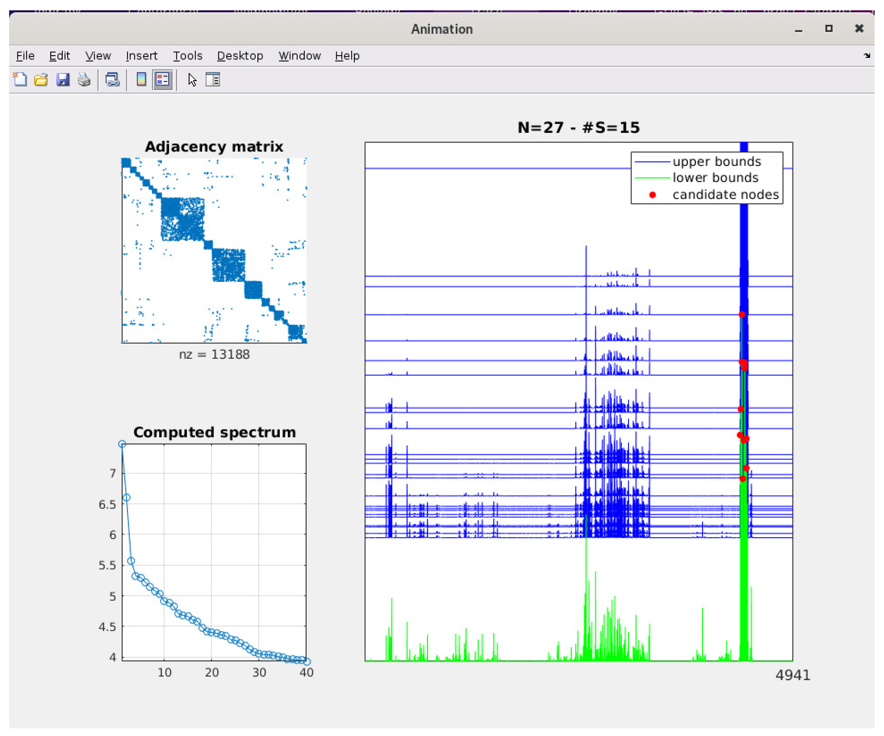
The first step to complete in order to carry out the computations is to load an adjacency matrix through the “File” menu at the top left of the main window. Once this task is done, general information about the network is shown, namely the number of nodes, the number of edges and, if the network contains self-loops, the number of removed edges. The parameters are set to their default values, and can be modified by the user. By pressing the “Find nodes” button the computations start. If the user chooses to show the animation (this possibility is not given if computation via Gauss quadrature is selected), a new window “Animation” will appear. It contains a spy plot of the adjacency matrix associated to the network with the number of non-zero elements, i.e., the number of edges, shown at the bottom of the figure. Below, the spectrum of
A is drawn and the graph is updated once a new set of eigenvalues is computed. On the right, an animation with the computed lower and upper bounds when each new eigenpair is added to the sum (
13) is shown. If either the strong or weak convergence criteria are satisfied, then the candidate nodes are highlighted with red circles. The title of the last graph reports the number of used eigenpair and the cardinality of the set
defined in (
16).
Figure 2 shows a typical animation window. In this case, the computations aim to identify the five most important nodes with respect to the subgraph centrality of the power network included in the package. The computations were carried out by the low-rank method with the strong convergence condition. The number of computed eigenpairs is the minimal integer
N such that the cardinality of
is 5.
Figure 3 shows the same window after identifying the same number of nodes as in
Figure 2 by the hybrid method. In this case, the cardinality of the set
is larger than 5, and the final computation to identify the five most important nodes is performed by Gauss quadrature.
Once the computations are made, the main window shows the following information:
the method used to perform the computation (low-rank with strong convergence, hybrid method or Gauss quadrature);
the line of code that has to be written on the command window to perform the same computation without using the graphical user interface;
whether the strong or weak convergence criteria are satisfied (if one of them was selected);
the number of used eigenpairs (if either the low-rank or hybrid methods have been used for the computations);
the number of VIP nodes identified (if either the low-rank or hybrid methods have been used);
the elapsed time;
a table with the index of the identified nodes and the value of the corresponding centrality index.
Figure 4 shows the main window once the computations related to
Figure 2 have been carried out.
Figure 5 shows the same window after the hybrid method has been used.
Please note that the lists of nodes produced by the two methods is the same, but the values of the centrality index are slightly different. This happens because the value of the subgraph centrality computed by the low-rank approximation is estimated as an average of the lower and upper bounds computed by the method, while the value computed by Gauss quadrature is more accurate.
6. Numerical Experiments
This section provides some numerical experiments to explore the performance of the centrality indices used in the software, namely the f-subgraph centrality and the f-starting convenience. In particular, we compare them to the following well-known centrality indices:
degree: the number of edges adjacent to a node;
betweeness: the number of shortest paths that pass through the node;
closeness: the reciprocal of the sum of the length of the shortest paths between a node and all other nodes in the graph;
eigenvector: a score is assigned to each node taking into account connections with nodes that have high scores;
pagerank: a variant of the eigenvector centrality.
The computation of the centrality indices listed above has been done by the centrality function included in Matlab. An example of its usage it is the following:
centr = ’betweenness’; % the centrality to be used
nnodes = 5; % the number of nodes to be identified
G = graph(A); % converts the adjacency matrix A in to the graph G
values = centrality(G,centr); % computes all the centralities of graph G
[∼, node_ind] = sort(values,’descend’); % sorts all the centralities
disp(node_ind(1:nnodes)); % displays the index for the nodes with the largest centrality
The string centr can be set to degree, betweenness, closeness, eigenvector, and pagerank.
The first network we analyze is the famous Zachary’s karate club network [
27]. The most important nodes of the network are node 1 and node 34, which stand for the instructor and the club president, respectively.
Each column of
Table 3 reports the ranking of the five most important nodes obtained using the centrality indices listed above, namely degree, betweenness, closeness, eigenvector, and pagerank centralities, compared with the ranking obtained by the
-subgraph centrality, the
-subgraph centrality, the
-starting convenience, and the
-starting convenience. The value used for
in (
3) is
. We remark that for this example, the ranking is not very sensitive to the choice of the parameter
.
It is worth noting that all the centrality indices correctly identify nodes 1 and 34 as the most important ones. The list of the five most important nodes contains the same indices except for the betweeness centrality, which includes in the list node 32, and the closeness centrality, which determines that node 32 and 9 are among the five most important nodes.
The second example we are going to consider is the Facebook network included in the package. The graph has 63,731 nodes and 1,545,686 edges. Neither the exponential nor the resolvent of the adjacency matrix
A can be evaluated in a straightforward manner due to the large size of the matrix. We therefore apply the hybrid algorithm described in
Section 4 to find the 10 most important nodes in the network.
Table 4 reports in each column the ranking of the 10 most important nodes according to the centrality indices described above and computed by the
centrality function of Matlab.
Table 5 reports the ranking of the 10 most important nodes obtained by the
-subgraph, the
-subgraph, the
-starting convenience and the
-starting convenience. The value used for
in (
3) is
and
.
It can be seen that the considered centrality indices generally produce different rankings. This confirms that they measure different features of the nodes in a network. It is remarkable to observe that in this example the -subgraph centrality and the -starting convenience produce the same list as the eigenvector centrality.


