1. Introduction
Sparse learning has emerged as a central topic of study in a variety of fields that require high-dimensional data analysis. Sparsity-constrained statistical models exploit the fact that high dimensional data arising from real-world applications frequently have low intrinsic complexity and have been shown to perform accurate estimation and inference in a variety of data mining fields, such as bioinformatics [
1], image analysis [
2,
3], graph sparsification [
4] and engineering [
5]. These models often require solving the following optimization problem with a nonconvex, nonsmooth sparsity constraint:
where
is a smooth and convex cost function in terms of a vector of parameters to be optimized
x,
denotes the
-norm (cardinality) of
x, which computes the number of nonzero entries in
x, and
is the sparsity level pre-specified for
x. Examples of this model include sparsity-constrained linear/logistic regression problems [
6,
7] and sparsity-constrained graphical models [
8].
Extensive research has been conducted for Problem (1). The methods largely fall into the regimes of either matching pursuit methods [
9,
10,
11,
12] or iterative hard thresholding (IHT) methods [
13,
14,
15]. Even though matching pursuit methods achieve remarkable success in minimizing quadratic loss functions (such as the
-constrained linear regression problems), they require finding an optimal solution to
min over the identified support after hard thresholding at each iteration, which lacks analytical solutions for arbitrary losses and can be time-consuming [
16]. Hence, gradient-based IHT methods have gained significant interest and become popular for nonconvex sparse learning. IHT methods currently include the gradient descent HT (GD-HT) [
14], stochastic gradient descent HT (SGD-HT) [
15], hybrid stochastic gradient HT (HSG-HT) [
17], and stochastic variance reduced gradient HT (SVRG-HT) [
18,
19] methods. These methods update the iterate
as follows:
, where
is the learning rate,
can be the full gradient, stochastic gradient or variance reduced gradient at the
t-th iteration, and
denotes the HT operator that preserves the top
elements in
x and sets other elements to 0. However, finding a solution to Problem (1) is generally NP-hard because of the non-convexity and non-smoothness of the cardinality constraint [
20].
Local datasets can be sensitive to sharing during the construction of a sparse inference model when sparse learning becomes distributed and uses data collected by distributed devices. For instance, meta-analyses may integrate genomic data from a large number of labs to identify (a sparse set of) genes contributing to the risk of a disease without sharing data across the labs [
21,
22]. Smartphone-based healthcare systems may need to learn the most important mobile health indicators from a large number of users; however, the personal health information gathered on the phone is private [
23]. Furthermore, communication efficiency can be the main challenge to distributively training a sparse learning model. Due to the power and bandwidth limitations of various sensors, the signal processing community, for instance, has been seeking more communication-efficient methods [
24].
Federated learning (FL) is a recently proposed communication-efficient distributed computing paradigm that enables collaborations among a collection of clients while preserving data privacy on each device by avoiding the transmission of local data to the central server [
25,
26,
27]. Hence, sparse learning can benefit from the setting of federated learning. In this paper, we solve the federated nonconvex sparsity-constrained empirical risk minimization problem with decentralized data as follows:
where
is a smooth and convex function,
is the loss function of the
i-th client (or device) with weight
,
,
is the distribution of data located locally on the
i-th client, and
N is the total number of clients. It is thus desirable to solve Problem (2) in a communication-efficient way and investigate theory and algorithms applicable to a broader class of sparse constrained learning problems in high-dimensional data analyses [
6,
7,
8,
28].
We thus propose federated HT algorithms with lower communication costs and provide the corresponding theoretical analysis under practical federated settings. The analysis of proposed methods is difficult due to the fact that distributions of training data on each client may be non-identical and the data weights can be unbalanced across devices.
Our main contributions are summarized as follows.
(a) We develop two schemes for the federated HT method: the Federated Hard Thresholding (Fed-HT) algorithm and Federated Iterative Hard Thresholding (FedIter-HT) algorithm. In Fed-HT, we apply the HT operator at the central server right before distributing the aggregated model to clients. To further improve the communication efficiency and the ability of sparsity recovery, in FedIter-HT, we consider applying to both local updates and the central server aggregate. Note that this is the first trial to explore IHT algorithms under federated learning settings.
(b) We provide a set of theoretical results for the federated HT method, particularly of Fed-HT and FedIter-HT, under the realistic condition that the distributions of training data over devices can be unbalanced and non-independent and non-identical (non-IID), i.e., for , and are different. We prove that both algorithms enjoy a linear convergence rate and have a strong guarantee for sparsity recovery. In particular, Theorems 1 (for the Fed-HT) and 2 (for the FedIter-HT) show that the estimation error between the algorithm iterate and the optimal solution is upper bounded as: where is the initial guess of the solution, the convergence rate factor is related to the algorithm parameter K (the number of SGD steps on each device before communication), and the closeness between the pre-specified sparsity level and the true sparsity , and determines a statistical bias term related not only to K but also to the gradient of f at the sparse solution and the measurement of the non-IIDness of the data across the devices.
The theoretical results allow us to evaluate and compare the proposed methods. For example, greater non-IIDness among clients increases the bias of both algorithms. More local iterations may reduce
but increase the statistical bias. Due to the utilization of the HT operator on local updates, the statistical bias induced by the FedIter-HT in Theorem 2 matches the best known upper bound for traditional IHT methods [
17], which exhibits the powerful capability of sparsity recovery.
(c) When instantiating the general loss function by concrete squared or logistic loss, we arrive at specific sparse learning problems, such as sparse linear regression and sparse logistic regression. We provide statistical analysis of the maximum likelihood estimators (M-estimators) of these problems when using the FedIter-HT to solve them. This result can be regarded as federated HT analysis for generalized linear models.
(d) Extensive experiments in simulations and on real-life datasets demonstrate the effectiveness of the proposed algorithms over standard distributed IHT learning.
2. Preliminaries
We formalize our problem as Problem (2) and provide the notations (
Table 1), assumptions and prepared lemmas used in this paper. We denote vectors by lowercase letters, e.g.,
x. The model parameters form a vector
. The
-norm,
-norm and the
-norm of a vector are denoted by
,
and
, respectively. Let
represent the asymptotic upper bound,
be the integer set
. The support
is associated with the
-th iteration in the
t-th round on device
i. For simplicity, we use
,
throughout the paper without ambiguity, and
.
We use the same conditions employed in the theoretical analysis of other IHT methods by assuming that the objective function satisfies the following conditions:
Assumption 1. We assume that the loss function on each device i
- 1.
is restricted -strongly convex (RSC [43]) at the sparsity level s for a given , i.e., there exists a constant such that with , , we have - 2.
is restricted -strongly smooth (RSS [43]) at the sparsity level s for a given , i.e., there exists a constant such that with , , we have - 3.
has -bounded stochastic gradient variance, i.e.,
Remark 1. When , the above assumption is no longer restricted to the support at a sparsity level, and is actually -strongly convex and -strongly smooth.
Following the same convention in FL [
35,
37], we also assume the dissimilarity between the gradients of the local functions
and the global function
f is bounded as follows.
Assumption 2. The functions () are -locally dissimilar, i.e., there exists a constant , such thatfor any . From the assumptions mentioned in the main text, we have the following lemmas to prepare for our theorems.
Lemma 1 ([
44]).
For and for any parameter , we havewhere and . Lemma 2. A differentiable convex function is restricted -strongly smooth with parameter s, i.e., there exists a generic constant such that for any , with andthen we have:The above two inequalities also hold for the global smoothness parameter . 3. The Fed-HT Algorithm
In this section, we first describe our new federated -norm regularized sparse learning framework via hard thresholding—Fed-HT, and then discuss the convergence rate of our proposed algorithm.
A high level summary of Fed-HT is described in Algorithm 1. The Fed-HT algorithm generates a sequence of
—sparse vectors
,
, ⋯, from an initial sparse approximation
. At the
-th round, clients receive the global parameter update
from the central server, then run
K steps of minibatch SGD based on local private data. In each step, the
i-th client updates
for
, i.e.,
. Clients send
for
back to the central server; then, the server averages them to obtain a dense global parameter vector and applies the HT operator to obtain a sparse iterate
. Unlike the commonly used FedAvg, the Fed-HT is designed to solve the family of federated
-norm regularized sparse learning problems. It has a strong ability to recover the optimal sparse estimator in decentralized non-IID and unbalanced data settings while at the same time reducing the communication cost by a large margin because the central server broadcasts a sparse iterate for each of the
T rounds.
| Algorithm 1. Federated Hard Thresholding (Fed-HT) |
Input: The learning rate , the sparsity level , and the number of clients N. Initialize for to do for client to N parallel do for to K do Sample uniformly a batch with batchsize end for end for end for
|
The following theorem characterizes our theoretical analysis of Fed-HT in terms of its parameter estimation accuracy for sparsity-constrained problems. Although this paper is focused on the cardinality constraint, the theoretical result is applicable to other sparsity constraints, such as a constraint based on matrix rank. Then, we have the main theorem and the detailed proof.
Theorem 1. Let be the optimal solution to Problem (2), , and suppose satisfies Assumptions 1 and 2. The condition number . Let stepsize and the batch size , , , , the sparsity level . Then the following inequality holds for the Fed-HT:where , , , . Note that if the sparse solution is sufficiently close to an unconstrained minimizer of , then is small, so the first exponential term on the right-hand side can be a dominating term, which approaches 0 when T goes to infinity. We further obtain the following corollary that bounds the number of rounds T to obtain a sub-optimal solution, i.e., the difference between the solution and is bounded only by the second term.
Corollary 1. If all the conditions in Theorem 1 hold, for a given precision , we need at most rounds to obtainwhere , , and . Remark 2. Corollary 1 indicates that under proper conditions and with sufficient rounds, the estimation error of the Fed-HT is determined by the second term—the statistical bias term—which we denote as . The term can become small if is sufficiently close to an unconstrained minimizer of , so it represents the sparsity-induced bias to the solution of the unconstrained optimization problem. The upper bound result guarantees that the Fed-HT can closely approach arbitrarily under a sparsity-induced bias, and the speed of approaching the biased solution is linear (or geometric) and determined by . In Theorem 1 and Corollary 1, is closely related to the number of local updates K. The condition number , so . When K is larger, is smaller, so is the number of rounds T required for reaching a target ϵ. In other words, the Fed-HT converges faster with fewer communication rounds. However, the bias term will increase when K increases. Therefore, K should be chosen to balance the convergence rate and statistical bias.
We further investigate how the objective function approaches the optimal .
Corollary 2. If all the conditions in Theorem 1 hold, let , and , we have Because the local updates on each device are based on SGD with dense parameters, without the HT operator, -smoothness and -strongly convexity are required, which depend on dimension d and are stronger requirements for f. Furthermore, , i.e., and are , which are suboptimal compared with the results for traditional IHT methods in terms of dimension d. In order to solve such drawbacks, we develop a new algorithm in the next section.
4. The FedIter-HT Algorithm
If we apply the HT operator to each local update as well, we obtain the FedIter-HT algorithm, as described in Algorithm 2. Hence, the local update on each device performs multiple SGD-HT steps, which further reduces the communication cost because model parameters sent back from clients to the central server are also sparse. If a client has a communication bandwidth so small that it can not effectively pass the full set of parameters, the FedIter-HT provides a good solution and also can relax the strict requirements for the objective function f and reduce the statistical bias. In this section, we first present a more communication-efficient federated -norm regularized sparse learning framework—FedIter-HT; then, we theoretically show it enjoys a better convergence rate compared with Fed-HT, and we further provide statistical analysis for M-estimators under the framework of FedIter-HT.
We again examine the convergence of the FedIter-HT by developing an upper bound on the distance between the estimator
and the optimal
, i.e.,
in the following theorem.
| Algorithm 2. Federated Iterative Hard Thresholding (FedIter-HT) |
Input: The learning rate , the sparsity level , and the number of clients N. Initialize for to do for client to N parallel do for to K do Sample uniformly a batch with batchsize end for end for end for
|
Theorem 2. Let be the optimal solution to (2), , and suppose satisfies Assumptions 1 and 2. The condition number . Let stepsize and the batch size , , , , the sparsity level . Then, the following inequality holds for the FedIter-HT:where , , , , , and . Remark 3. The factor , compared with in Theorem 1, is smaller if , which means that the FedIter-HT converges faster than the Fed-HT when the beforehand-guessed sparsity τ is much larger than the true sparsity. Both and will decrease when the number of internal iterations K increases, but decreases faster than because is smaller than . Thus, the FedIter-HT is more likely to benefit by increasing K than the Fed-HT. The statistical bias term can be much smaller than in Theorem 1 because only depends on the norm of restricted to the support of size . Because the norm of the gradient is a dominating term in and , slightly increasing K does not significantly vary the statistical bias terms (when ).
Using the results in Theorem 2, we can further derive Corollary 3 to specify the number of rounds required to achieve a given estimation precision.
Corollary 3. If all the conditions in Theorem 2 hold, for a given , the FedIter-HT requires the most rounds to obtainwhere . Because , and we also know and in high dimensional statistical problems, the result in Corollary 3 gives a tighter bound than the one obtained in Corollary 1. Similarly, we also obtain a tighter upper bound for the convergence performance of the objective function .
Corollary 4. If all the conditions in Theorem 2 hold, let , and , we have The theorem and corollaries developed in this section only depend on the -restricted smoothness and -restricted strong convexity, where , which are the same conditions used in the analysis of existing IHT methods. Moreover, , which means and are , where is the size of support . Therefore, our results match the current best-known upper bound for the statistic bias term compared with the results for traditional IHT methods.
5. Experiments
We empirically evaluate our methods in both simulations and on three real-world datasets: E2006-tfidf, RCV1 and MNIST (
Table 2, which are downloaded from the LibSVM website (
https://www.csie.ntu.edu.tw/~cjlin/libsvmtools/datasets/, accessed on 1 July 2022)), and compare them against a baseline method. The baseline method is a standard Distributed IHT and communicates every local update to the central server, which then aggregates and broadcasts back to clients (see
Appendix A.1 for more details). Specifically, experiments for simulation I and on the E2006-tfidf dataset are conducted for sparse linear regression. We solve the sparse logistic regression problem in simulation II and for the RCV1 data set. The last experiment uses MNIST data in a multi-class softmax regression problem. The exact loss functions for the various problems are available in the
Appendix A.2.
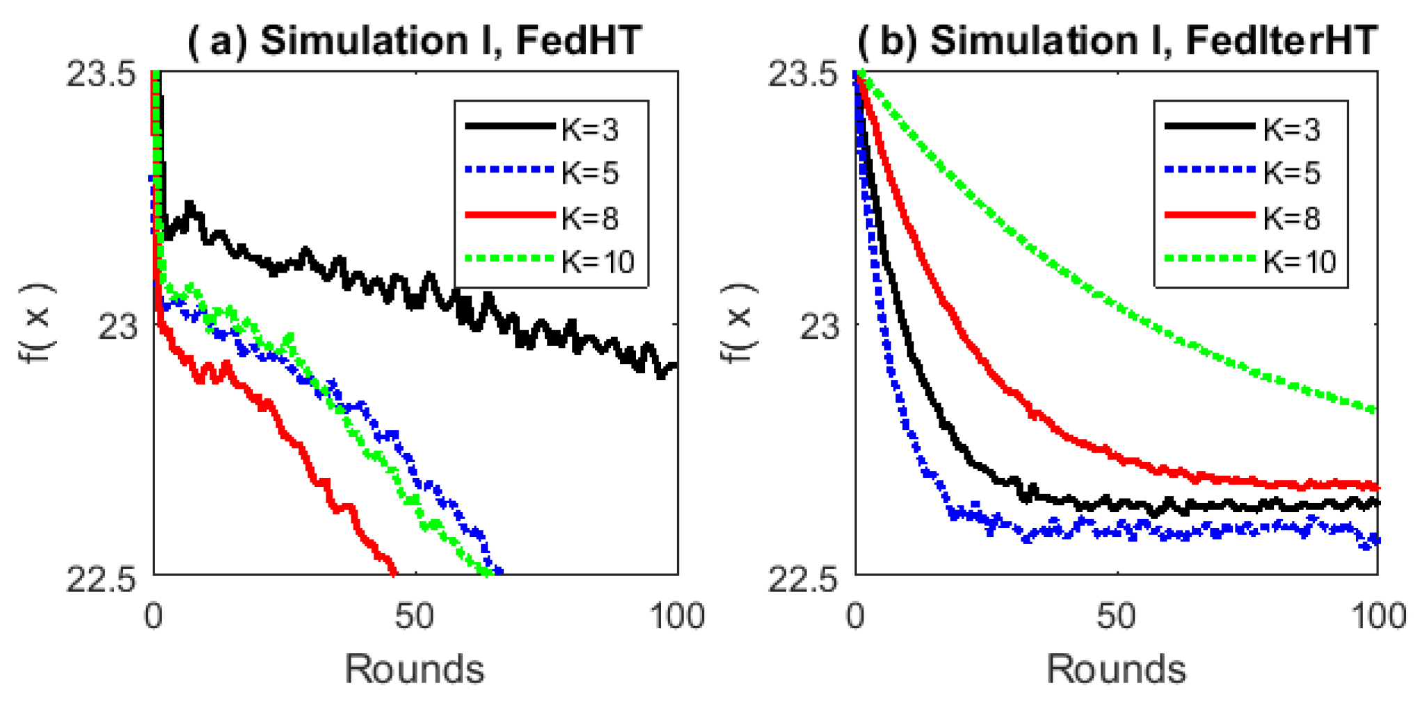
Following the convention in the federated learning literature, we use the number of communication rounds to measure the communication cost. For a comprehensive comparison, we also include the number of iterations. For both synthetic and real-world datasets, algorithm parameters are determined by the following criteria. The number of local iterations
K is searched from
. We have tested the performance of our proposed algorithms under different
K conditions (see
Figure 1). The stepsize
for each algorithm is set by a grid search from
. All the algorithms are initialized with
. The sparsity
is 500 for the MNIST dataset and 200 for the other two datasets.
5.1. Simulations
To generate synthetic data, we follow a similar setup to that in [
37]. In simulation I, for each device
, we generate samples
for
according to
, where
,
. The first 100 elements of
are drawn from
and the remaining elements in
are zeros,
,
,
, where
is a diagonal matrix with the
i-th diagonal element equal to
. Each element in the mean vector
is drawn from
,
. Therefore,
controls how much the local models differ from each other, and
controls how much the local on-device data differ between one another; hence, we have simulated Non-IID federated data. In simulation I,
. The data generation procedure for simulation II is the same as the procedure of simulation I, except that
; then, for the
i-th client, we set
corresponding to the top 100 of
for
; otherwise,
. In simulation II, we also set
.
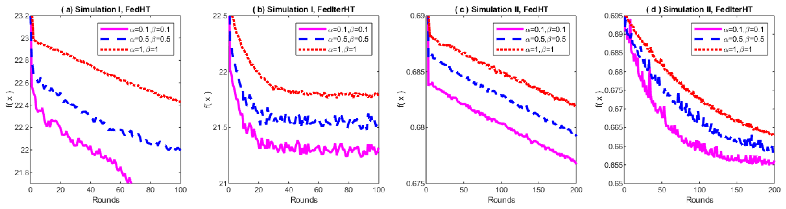
The results in
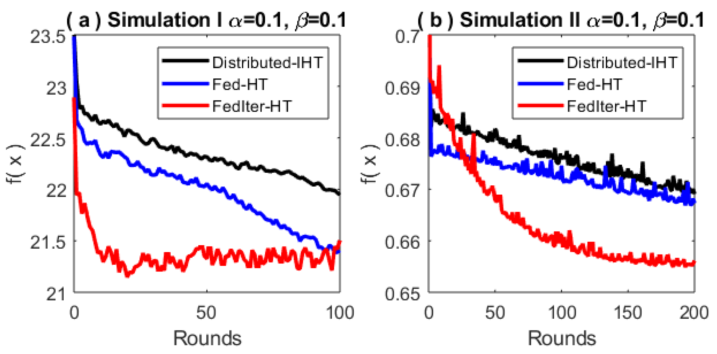
Figure 2 show that, with a higher degree of Non-IID, both Fed-HT and FedIter-HT tend to converge slower. We also compare the proposed methods with the baseline method—Distributed IHT. In
Figure 3, we observe that in simulation I, FedIter-HT only needs 20 (∼
less) communication rounds to reach the same objective value that the Distributed-IHT obtains with more than 100 communication rounds; in simulation II, the FedIter-HT needs 50 communication rounds (∼
less) to achieve the same objective value that the Distributed-IHT obtains with 200 communication rounds.
5.2. Benchmark Datasets
We use the E2006-tfidf dataset [
47] to predict the volatility of stock returns based on the SEC-mandated financial text report, represented by tf-idf. It was collected from thousands of publicly traded U.S. companies, for which data from different companies are inherently non-identical and the privacy consideration for financial data demands federated learning. The RCV1 dataset [
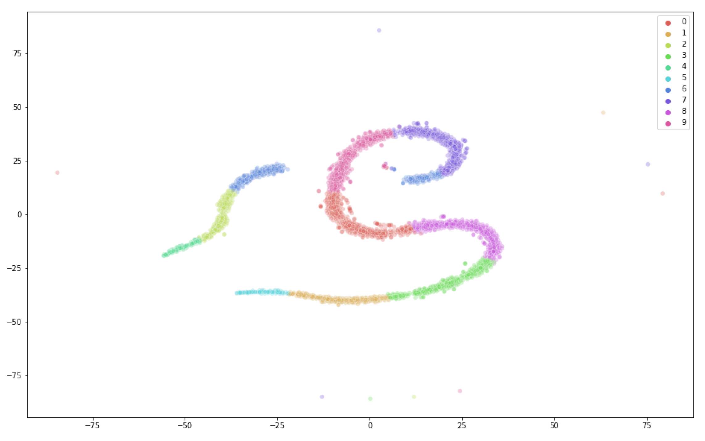
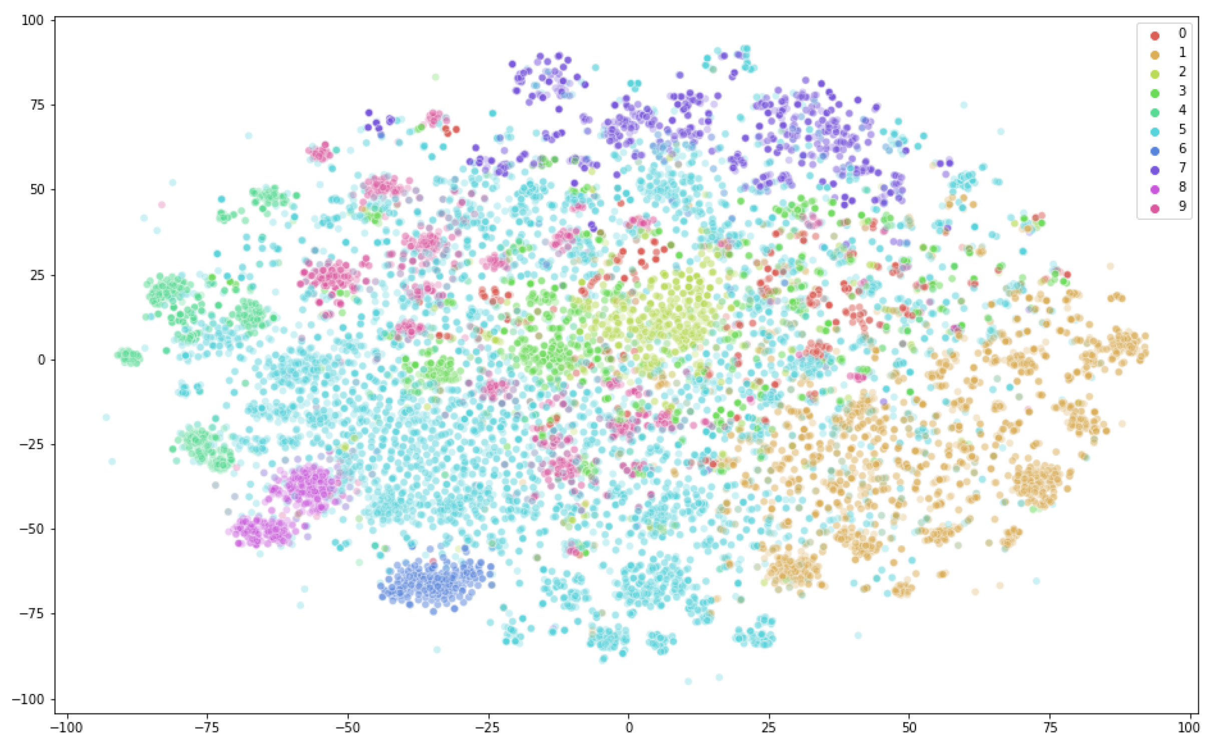
48] is used to predict categories of newswire stories recently collected by Reuters, Ltd. The RCV1 can be naturally partitioned based on the news category and used for federated learning experiments since readers may only be interested in one or two categories of news. Our model training process mimics the personalized privacy-preserving news recommender system where we use the K-means method to partition the datasets, respectively, into 10 clusters. Each device randomly selects two of the clusters for use in the learning. We run t-SNE to visualize the hidden structures found by K-means as shown in
Figure 4 and
Figure 5, respectively, for the E2006-tfidf dataset (sparse linear regression) and the RCV1 dataset (sparse logistic regression). For the MNIST images, there are 10 digits that automatically serve as the clusters.
For all datasets, the data in each cluster are evenly partitioned into 20 parts, and each client randomly picks two clusters and selects one part of data from each of the clusters. Because the MNIST images are evenly collected for each digit, the partitioned decentralized MNIST data are balanced in terms of categories, whereas the other two datasets are unbalanced.
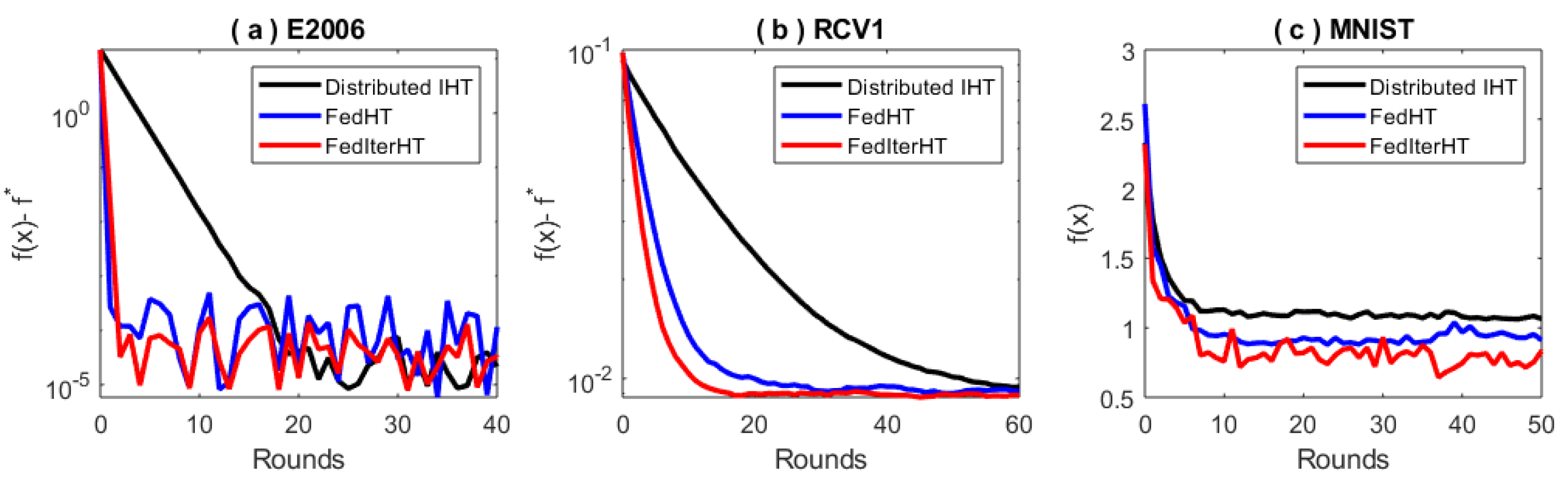
Figure 6 shows that our proposed Fed-HT and FedIter-HT can significantly reduce the communication rounds required to achieve a given accuracy. In
Figure 6a,c, we further notice that federated learning displays more randomness when approaching the optimal solution. This may be caused by dissimilarity across clients. For instance, the three different algorithms in
Figure 6c reach the neighborhood of different solutions at the end, where the proposed FedIter-HT obtains the lowest objective value. These behaviors may be worth exploring further in the future.


