Some Inexact Version of the Iterative Exponential Method for Solving Nonsmooth Equations

Abstract

This paper presents an inexact version of an exponential iterative method designed for solving nonlinear equations $F\left(x\right)=0$, where the function F is only locally Lipschitz continuous. The proposed algorithm is completely new as an essential extension of the iterative exponential method for solving nonsmooth equations. The method with backtracking is globally and superlinearly convergent under some mild assumptions imposed on F. The presented results of the numerical computations confirm both the theoretical properties of the new method and its practical effectiveness.

1. Introduction

Let $F:R^n\to R^n$ be locally Lipschitz continuous. Consider the nonlinear equation in the following simplest form:

$$F\left(x\right)=0,$$

(1)

where $x={(x_1,\dots ,x_n)}^T$, $F\left(x\right)={(f_1\left(x\right),\dots ,f_n\left(x\right))}^T$ and $f_i:R^n\to R$, $i=1,\dots ,n$. Furthermore, we assume that there exists $x^{\ast }\in R^n$, which is a solution to Equation (1) (i.e., $F\left(x^{\ast }\right)=0$). It is worth recalling that Pang and Qi [1] presented significant motivations and a broad scope of applications for nonsmooth equations.

Some class of iterative exponential methods for solving one-dimensional nonlinear equations was proposed by Chen and Li [2]. One of the most interesting formulas, and simultaneously the simplest one, is the method which has the following form:

$$x_{k+1}=x_{k}exp\left\{-\frac{f\left(x_k\right)}{x_k{f}^{\prime }\left(x_k\right)}\right\},k=0,1,2,\dots$$

(2)

This method turns to the classic Newton method if we use the first-order Taylor series expansion of the expression $exp\left\{-\frac{f\left(x_k\right)}{x_k{f}^{\prime }\left(x_k\right)}\right\}$. The above method in Equation (2) has (at least) quadratic convergence if the function $f:R\to R$ is twice differentiable and $f^{\prime }\left(x\right)\ne 0$ in a neighborhood of the solution. A substantial extension of the exponential method in Equation (2) to the nonsmooth case in $R^n$ was presented in [3]. This locally and superlinearly convergent method can be written in the following two-stage form:

$$\left\{\begin{array}{c}{V}_k{h}^{\left(k\right)}=-F\left(x^{\left(k\right)}\right)\hfill \\ x^{(k+1)}=\mathrm{diag}\left(exp\left\{\frac{h_i^{\left(k\right)}}{x_i^{\left(k\right)}}\right\}\right)x^{\left(k\right)}\hfill \end{array}\right.$$

(3)

where the matrix $V_k$ is arbitrarily taken from the B-differential of F at $x^{\left(k\right)}$.

On the other hand, one traditional approach for solving nonsmooth equations is the inexact generalized Newton method:

$$∥F\left(x^{\left(k\right)}\right)+V_k{h}^{\left(k\right)}∥\le {\eta }_k∥F\left(x^{\left(k\right)}\right)∥,$$

(4)

where the matrix $V_k$ could be arbitrarily taken from some subdifferential of F at $x^{\left(k\right)}$ (not only from the generalized Jacobian or B-differential but also from, for example, the ∗-differential) and $0\le {\eta }_k<1$ for all $k=0,1,2,\dots$ Martínez and Qi in [4] stated the local and superlinear convergence of the generalized Jacobian-based method with Equation (4) for solving equations with semismooth function F. Other versions of such Newton-type methods for solving nonsmooth equations were also considered among the others in [5,6,7]. The main concept of the inexact Newton-type method is to substitute the standard Newton equation $V_k{h}^{\left(k\right)}=-F\left(x^{\left(k\right)}\right)$ with an inequality as in Equation (4), where the parameter ${\eta }_k\in [0,1)$ is the forcing term. Then, the Newton step $h_k$ may be determined inexactly, such as by the use of any iterative method with feasible inaccuracy, especially when the current approximation is far from the solution to Equation (1).

The main objective of this paper is to introduce an inexact version of the exponential method with a subdifferential for multidimensional nonsmooth cases. Therefore, we present some new iterative methods for solving nondifferentiable problems, which can be sufficiently effective in solving not only nonsmooth equations but also some important problems in nonsmooth optimization. The exponential method was introduced in [2] for finding single roots of univariate nonlinear equations and considered in [8] for solving unconstrained optimization problems. In both cases, the proposed formulas allow solving only smooth and one-dimensional problems. We discuss an algorithm which is intended to solve both nonsmooth and multi-dimensional problems. Our method allows solving Equation (1), in which the function is only Lipschitz continuous and need not be differentiable. A primary extension, shown in Equation (3), was introduced in [3], but this study focuses on the inexact approach. In this way, vector $h^{\left(k\right)}$ can be approximated in every iteration with some inaccuracy, which reduces the cost of determining it. However, all these methods are only locally convergent. A new approach also includes a backtracking procedure, and as a result, we obtained a global convergence of the inexact exponential method.

This paper is organized as follows. We recall some important needed notions and properties in Section 2. In Section 3, we not only introduce an algorithm but also prove its global and superlinear convergence. Section 4 features the results of numerical tests. In Section 5 at the end, we give some conclusions.

2. Preliminaries

Throughout the paper, $∥·∥$ denotes the Euclidean norm on $R^n$, where we regard the vector from $R^n$ as a column vector. However, all theoretical results do not depend on the choice of the norm.

We assume that the function F is locally Lipschitz continuous in the traditional sense. In other words, for every $U\subset R^n$, there exists a constant $L>0$ such that

$$∥F\left(x\right)-F\left(y\right)∥\le L∥x-y∥ \mathrm{for} \mathrm{all} x,y\in U.$$

If $F:R^n\to R^n$ is a differentiable function, we denote the Jacobian matrix of F at x as $JF\left(x\right)$ and the set where F is differentiable as $D_F$. The local Lipschitz continuity of the function F implies that it is differentiable almost everywhere, according to Rademacher’s theorem [9]. Then, we have

$${\partial }_{B}F\left(x\right)=\left\{\underset{x_i\to x}{lim}JF\left(x_i\right),x_i\in D_F\right\}$$

which is called the Bouligand subdifferential (B-differential for short) of F at x [10]. Furthermore, the generalized Jacobian of function F at x (in the sense of Clarke [9]) is the convex hull of the Bouligand subdifferential such that

$$\partial F\left(x\right)=\mathrm{conv}{\partial }_{B}F\left(x\right).$$

We say that the function F is BD-regular at x if F is locally Lipschitz continuous at x and if all matrices V from ${\partial }_{B}F\left(x\right)$ are nonsingular. For BD-regular functions, Qi proved some important properties (see Lemma 2).

In turn, the set

$${\partial }_{b}F\left(x\right)={\partial }_B{f}_1\left(x\right)\times \dots \times {\partial }_B{f}_n\left(x\right),$$

is called the b-differential of function F at x (defined by Sun and Han in [11]). It is easy to verify that in a one-dimensional case (i.e., when $n=1$), the generalized Jacobian reduces to the Clarke generalized gradient and ${\partial }_{B}F\left(x\right)={\partial }_{b}F\left(x\right)$ i.e., the B-differential and b-differential coincide). Furthermore, a ∗-differential ${\partial }_{\ast }F\left(x\right)$ is a non-empty bounded set for any x such that

$${\partial }_{\ast }F\left(x\right)\subset \partial f_1\left(x\right)\times \dots \times \partial f_n\left(x\right),$$

where $\partial f_i\left(x\right)$ denotes the generalized gradient of the component function $f_i$ at x. Obviously, for a locally Lipschitz function, all previously mentioned differentials, namely $\partial F\left(x\right)$, ${\partial }_{B}F\left(x\right)$ and ${\partial }_{b}F\left(x\right)$, are ∗-differentials (see Gao [12]). Obviously, if all components $f_i$ of function F are $C^1$ at x, then $\partial F\left(x\right)={\partial }_{B}F\left(x\right)=\left\{JF\left(x\right)\right\}$.

The notion of semismoothness was primarily introduced by Mifflin [13] for functionals. Later, Qi and Sun [14] extended the original definition to nonlinear operators. A function F is semismooth at x if F is locally Lipschitz continuous at x and for any $h\in R^n$, the limit

$$\underset{V\in \partial F(x+t{h}^{\prime }),h^{\prime }\to h,t\downarrow 0}{lim}V{h}^{\prime }.$$

exists. If function F is semismooth at x, then F is directionally differentiable at x, and $F^{\prime }(x;h)$ is equal to the above limit:

Lemma 1

(Lemma 2.2 by Qi [15]). Suppose that the function $F:R^n\to R^n$ is directionally differentiable in a neighborhood of x. The following statements are equivalent:

(1) 

F is semismooth at x;

(2) 

$F^{\prime }(·,·)$ is semicontinuous at x;

(3) 

For any $V\in \partial F(x+h)$, the following is true:

$$Vh-F^{\prime }(x;h)=o\left(∥h∥\right) \mathrm{as} h\to 0.$$

Moreover, we say that function F is p-order semismooth at x if for any matrix V from the generalized Jacobian $\partial F(x+h)$, it holds that

$$Vh-F^{\prime }(x,h)=O\left({∥h∥}^{1+p}\right)\mathrm{as} h\to 0,$$

where $0<p\le 1$. If $p=1$, then F is just called strongly semismooth [16].

Remark 1.

(i) 

Clearly, semismoothness of any order implies semismoothness.

(ii) 

The piecewise $C^2$ function is strongly semismooth.

Lemma 2

(Lemma 2.6 by Qi [15]). If function F is BD-regular at x, then there is a neighborhood N of x and a constant $C>0$ such that for any $y\in N$ and matrix $V\in {\partial }_{B}F\left(y\right)$, V is nonsingular, and

$$∥V^{-1}∥\le C.$$

If the function F is also semismooth at $y\in N$, then for any $h\in R^n$, the following is true:

$$∥h∥\le C∥F^{\prime }\left(y;h\right)∥.$$

Qi and Sun showed in [14] that if a function F is semismooth at x, then

$$F(x+h)-F\left(x\right)-F^{\prime }(x;h)=o\left(∥h∥\right) \mathrm{for} \mathrm{any} h\to 0.$$

(5)

Furthermore, if a function F is p-order semismooth at x, then

$$F(x+h)-F\left(x\right)-F^{\prime }(x;h)=O\left({∥h∥}^{1+p}\right) \mathrm{for} \mathrm{any} h\to 0.$$

(6)

Throughout this paper, $N(x,r)$ denotes the closed ball with a center x and radius r in $R^n$ (if the center is known, and a radius is negligible, just N is used).

Furthermore, for a given diagonal matrix whose diagonal entries are $d_1,\dots ,d_n$ such that

$$D=\mathrm{diag}(d_1,\dots ,d_n)=\left[\begin{array}{cccc}{d}_1& 0& \dots & 0\\ 0& d_2& \dots & 0\\ \dots & \dots & \dots & \dots \\ 0& 0& \dots & d_n\end{array}\right],$$

then $exp\left(D\right)$ denotes a so-called exponential matrix, which has the following form:

$$exp\left(D\right)=\left[\begin{array}{cccc}{e}^{d_1}& 0& \dots & 0\\ 0& e^{d_2}& \dots & 0\\ \dots & \dots & \dots & \dots \\ 0& 0& \dots & e^{d_n}\end{array}\right].$$

3. The Algorithm and Its Properties

In this section, we introduce a new algorithm, and we discuss its convergence. For solving Equation (1), we can consider a method in the descriptive two-stage form

$$\left\{\begin{array}{c}\mathrm{determine} h^{\left(k\right)}\mathrm{using} V_k\mathrm{and} F\left(x^{\left(k\right)}\right)\hfill \\ \mathrm{compute} x^{(k+1)}\mathrm{using} x^{\left(k\right)}\mathrm{and} h^{\left(k\right)}\hfill \end{array}\right.$$

where matrix $V_k$ is taken from some subdifferential of F at $x^{\left(k\right)}$. We suggest an approach which is a combination of two methods: the iterative exponential one and the inexact generalized Newton one with a decreasing function norm and backtracking. The proposed inexact approach is similar to the algorithm presented by Birgin et al. [17] for smooth equations, whereas the exponential formula was introduced in [3]. Because of the nondifferentiability of F, as iteration matrices, we use matrices from the B-differential instead of the Jacobians.

Remark 2.

(i) 

The matrix $V_k$ may be chosen absolutely arbitrarily from known elements of the Bouligand subdifferential (in Step 1 of Algorithm 1). Appropriate matrices are usually suitable Jacobians of F.

(ii) 

The backtracking approach used in Step 2 is a particular case of the minimum reduction algorithm.

(iii) 

The formula in Equation (10) for obtaining $x^{(k+1)}$ could be written in a substitute form, which explicitly shows how to generate a new approximation $x^{(k+1)}$ using components of the previous approximation $x^{\left(k\right)}$:

$$x_i^{(k+1)}=x_i^{\left(k\right)}exp\left\{\frac{{\alpha }_k{h}_i^{\left(k\right)}}{x_i^{\left(k\right)}}\right\},i=1,\dots ,n.$$

(7)

(iv) 

Various strategies for the choice of the forcing sequence can be found in [18] but for the inexact methods for solving smooth equations. Therefore, most of these strategies would need to be modified with respect to the nondifferentiability of F. For example, we could set ${\eta }_k\in [0,1)$ as a small constant or use the following rule:

$${\eta }_k=\left\{\begin{array}{cc}\frac{∥V_k{h}^{\left(k\right)}+F\left(x^{\left(k\right)}\right)∥}{∥F\left(x^{\left(k\right)}\right)∥}\hfill & \mathrm{if} F\left(x^{\left(k\right)}\right)\ne 0\\ 0\hfill & \mathrm{otherwise},\end{array}\right.$$

where $V_k\in {\partial }_{B}F\left(x^{\left(k\right)}\right)$. Then, Equation (8) holds with equality.

Before the convergence of Algorithm 1 is proven, we present a necessary important assumption:

Algorithm 1: Inexact exponential method (IEM).

Assume that $\theta \in \left(0,1\right)$, ${\tau }_1,{\tau }_2\in \left(0,1\right)$ and ${\tau }_1<{\tau }_2$. Let $x^{\left(0\right)}\in R^n$ be an arbitrary starting approximation. The steps for obtaining $x^{(k+1)}$ from $x^{\left(k\right)}$ are as follows: Step 1: Determine ${\eta }_k\in \left[0,1\right)$ and find an $h^{\left(k\right)}$ value that satisfies $$∥V_k{h}^{\left(k\right)}+F\left(x^{\left(k\right)}\right)∥\le {\eta }_k∥F\left(x^{\left(k\right)}\right)∥,$$ (8) where $V_k\in {\partial }_{B}F\left(x^{\left(k\right)}\right)$. Set $\alpha =1$. Step 2: If $$∥F\left(\mathrm{diag}\left(exp\left\{\frac{\alpha h_i^{\left(k\right)}}{x_i^{\left(k\right)}}\right\}\right)x^{\left(k\right)}\right)∥\le \left[1-\alpha \theta \left(1-{\eta }_k\right)\right]∥F\left(x^{\left(k\right)}\right)∥$$ (9) then set ${\alpha }_k=\alpha$ and $$x^{(k+1)}=\mathrm{diag}\left(exp\left\{\frac{{\alpha }_k{h}_i^{\left(k\right)}}{x_i^{\left(k\right)}}\right\}\right)x^{\left(k\right)}.$$ (10) Otherwise, choose ${\alpha }^{\prime }\in \left[{\tau }_1\alpha ,{\tau }_2\alpha \right]$, set $\alpha ={\alpha }^{\prime }$, and repeat Step 2.

Assumption 1.

Function F satisfies Assumption 1 at x if for any y from a neighborhood N of x and any matrix $V_y\in {\partial }_{B}F\left(y\right)$, it holds that

$$F\left(y\right)-F\left(x\right)=V_y\left(y-x\right)+o\left(∥y-x∥\right).$$

Furthermore, function F satisfies Assumption 1 at x with a degree ρ if the following holds:

$$F\left(y\right)-F\left(x\right)=V_y\left(y-x\right)+O\left({∥y-x∥}^{\rho }\right).$$

Remark 3.

(i) 

It is not difficult to indicate functions that satisfy Assumption 1. We can indicate three classes of such functions. Assumption 1 is implied not only by semismoothness but also by H-differentiability (introduced by Song et al. [19]) and second-order C-differentiability (introduced by Qi [10]).

(ii) 

If function F is BD-regular at x and satisfies Assumption 1 at x, then there is a neighborhood N of x and a constant $C>0$ such that for any $y\in N$ and matrix $V\in {\partial }_{B}F\left(y\right)$, the following is true:

$$∥y-x∥\le C∥V_y\left(y-x\right)∥.$$

(11)

(iii) 

Lemma 2, proven in [7], states that if function F is BD-regular at $x^{\ast }$, satisfies Assumption 1 at $x^{\ast }$ and $l=max\left\{2\beta ,\frac{1}{2\beta }+∥V_y∥\right\}$, where $\beta =∥V_y^{-1}∥$ and $V_y\in {\partial }_{B}F\left(y\right)$, then

$$\frac{1}{l}∥y-x^{\ast }∥\le ∥F\left(y\right)∥\le l∥y-x^{\ast }∥\mathrm{for} \mathrm{all} y\in N,$$

where N is a neighborhood of $x^{\ast }$.

Now, we establish some theoretical foundations for Algorithm 1:

Lemma 3.

Assume that Algorithm 1 is carried out with ${\eta }_k\in \left(0,1\right)$ determined in such way that the inequality in Equation (9) holds. If the series ${\sum }_{k=1}^{\infty }\left(1-{\eta }_k\right)$ is divergent, then

$$\underset{k\to \infty }{lim}F\left(x^{\left(k\right)}\right)=0.$$

Proof of Lemma 3.

Under Equation (9), the following is true:

$$\begin{array}{ccc}∥F\left(x^{\left(k\right)}\right)∥\hfill & \le \hfill & \left[1-\alpha \theta \left(1-{\eta }_k\right)\right]∥F\left(x^{(k-1)}\right)∥\hfill \\ \hfill & \le \hfill & ∥F\left(x^{\left(0\right)}\right)∥\prod _{0\le j<k}[1-\alpha \theta (1-{\eta }_k)]\hfill \\ \hfill & \le \hfill & ∥F\left(x^{\left(0\right)}\right)∥exp\left\{-\alpha \theta \sum _{0\le j<k}(1-{\eta }_k)\right\}\hfill \end{array}$$

Since $1-{\eta }_k\ge 0$ and $\alpha \theta >0$, convergence $F\left(x^{\left(k\right)}\right)$ to 0 follows from the divergence of ${\sum }_{k\ge 0}(1-{\eta }_k)$. □

The divergence of series ${\sum }_{k=1}^{\infty }\left(1-{\eta }_k\right)$ implies a satisfactory decrease in $∥F∥$ over all steps such that $F\left(x^{\left(k\right)}\right)\to 0$, namely if the inequality in Equation (9) holds.

Lemma 4.

Let $\theta \in \left(0,1\right)$ and x be given, and assume that there is $\overline{h}$, which satisfies $∥V\overline{h}+F\left(x\right)∥<∥F\left(x\right)∥$, where $V\in {\partial }_{B}F\left(x\right)$. If function F satisfies Assumption 1 at x, then there is ${\eta }_{min}\in \left[0,1\right)$ such that for any $\eta \in \left[{\eta }_{min},1\right)$, there exists h, which satisfies

$$∥Vh+F\left(x\right)∥\le \eta ∥F\left(x\right)∥ \mathrm{and} ∥F\left(\mathrm{diag}\left(exp\left\{\frac{\alpha h_i}{x_i}\right\}\right)x\right)∥\le \left[1-\alpha \theta \left(1-\eta \right)\right]∥F\left(x\right)∥,$$

where $\alpha \in \left(0,1\right]$.

Proof of Lemma 4.

Obviously, $F\left(x\right)\ne 0$ and $\overline{h}\ne 0$.

Set

$$\begin{array}{ccc}\overline{\eta }\hfill & =\hfill & \frac{∥V\overline{h}+F\left(x\right)∥}{∥F\left(x\right)∥},\hfill \\ {\eta }_{min}\hfill & =\hfill & max\left\{\overline{\eta },1-\frac{\left(1-\overline{\eta }\right)\delta }{∥\overline{h}∥}\right\},\hfill \\ ϵ\hfill & =\hfill & \frac{\left(1-\alpha \theta \right)\left(1-\overline{\eta }\right)∥F\left(x\right)∥}{∥\overline{h}∥},\hfill \end{array}$$

where $\delta >0$ is sufficiently small for the following inequality to be satisfied:

$$∥F\left(\mathrm{diag}\left(exp\left\{\frac{\alpha h_i}{x_i}\right\}\right)x\right)-F\left(x\right)-Vh∥\le ϵ∥h∥,$$

whenever $∥h∥\le \alpha \delta$. Under Assumption 1, such a value of $\delta$ exists. Since $\overline{\eta }<1$, then ${\eta }_{min}<1$.

Let

$$h=\frac{1-\eta }{1-\overline{\eta }}\overline{h}$$

for any $\eta \in \left[{\eta }_{min},1\right)$. Then, we have

$$\begin{array}{ccc}∥Vh+F\left(x\right)∥\hfill & =\hfill & \frac{∥\left(1-\eta \right)V\overline{h}+\left(1-\overline{\eta }\right)F\left(x\right)∥}{1-\overline{\eta }}\hfill \\ \hfill & \le \hfill & \frac{1-\eta }{1-\overline{\eta }}∥V\overline{h}+F\left(x\right)∥+\frac{\eta -\overline{\eta }}{1-\overline{\eta }}∥F\left(x\right)∥\hfill \\ \hfill & =\hfill & \frac{1-\eta }{1-\overline{\eta }}\overline{\eta }∥F\left(x\right)∥+\frac{\eta -\overline{\eta }}{1-\overline{\eta }}∥F\left(x\right)∥\hfill \\ \hfill & =\hfill & \eta ∥F\left(x\right)∥.\hfill \end{array}$$

In addition, since

$$∥h∥=\frac{1-\eta }{1-\overline{\eta }}∥\overline{h}∥\le \frac{1-{\eta }_{min}}{1-\overline{\eta }}∥\overline{h}∥\le \delta ,$$

then

$$\begin{array}{ccc}\hfill & \hfill & ∥F\left(\mathrm{diag}\left(exp\left\{\frac{\alpha h_i}{x_i}\right\}\right)x\right)∥\hfill \\ \hfill & \le \hfill & ∥F\left(\mathrm{diag}\left(exp\left\{\frac{\alpha h_i}{x_i}\right\}\right)x\right)-F\left(x\right)-Vh∥+∥Vh+F\left(x\right)∥\hfill \\ \hfill & \le \hfill & ϵ\frac{1-\eta }{1-\overline{\eta }}∥\overline{h}∥+\eta ∥F\left(x\right)∥\hfill \\ \hfill & =\hfill & \left(1-\alpha \theta \right)\left(1-\eta \right)∥F\left(x\right)∥+\eta ∥F\left(x\right)∥\hfill \\ \hfill & =\hfill & \left[1-\alpha \theta \left(1-\eta \right)\right]∥F\left(x\right)∥.\hfill \end{array}$$

□

Lemma 4 above implies that the inexact exponential step is well-defined for the current approximation $x^{\left(k\right)}$, and suitable ${\eta }_k$ and $h^{\left(k\right)}$ values exist for any $\theta \in \left(0,1\right)$.

Now, we will prove that the method described by Algorithm 1 is convergent. The first theorem regarding convergence is analogous to the one presented in [20] for the inexact generalized Newton method for solving nonsmooth equations, albeit with some significant changes in the proof:

Theorem 1.

Let $\left\{x^{\left(k\right)}\right\}$ be a sequence generated by Algorithm 1 with ${\eta }_k\to 0$, and for each k, there is a constant $M>0$ such that the following holds:

$$∥V_k{h}^{\left(k\right)}+F\left(x^{\left(k\right)}\right)∥\le {\eta }_k∥F\left(x^{\left(k\right)}\right)∥$$

and

$$∥h^{\left(k\right)}∥\le M$$

for any matrix $V_k\in {\partial }_{B}F\left(x^{\left(k\right)}\right)$.

If function F satisfies Assumption 1 at $x^{\ast }$, then every limiting point of the sequence $\left\{x^{\left(k\right)}\right\}$ is a solution to Equation (1), and

$$\underset{k\to \infty }{lim}F\left(x^{\left(k\right)}\right)=0.$$

Proof of Theorem 1.

Suppose that K is a sequence of indices such that ${lim}_{k\in K}{x}^{\left(k\right)}=x^{\ast }$. We have two cases due to the behavior of the sequence $\left\{{\alpha }_k\right\}$:

(i)

$\left\{{\alpha }_k\right\}$ is not convergent to 0.

Then, there is a sequence of indices $K_0\subset K$ and $\overline{\alpha }>0$ such that ${\alpha }_k\ge \overline{\alpha }>0$ for all $k\in K_0$. Clearly, for all $k\notin K_0$, the following is true:

$$∥F\left(x^{(k+1)}\right)∥\le ∥F\left(x^{\left(k\right)}\right)∥.$$

In turn, according to Equation (9), we have

$$∥F\left(x^{(k+1)}\right)∥\le ∥F\left(x^{\left(k\right)}\right)∥-\overline{\alpha }\theta \left(1-{\eta }_k\right)∥F\left(x^{\left(k\right)}\right)∥ \mathrm{for} \mathrm{all} k\in K_0.$$

By adding all these inequalities side by side, we obtain the following inequality:

$$\overline{\alpha }\theta \sum _{k\in K_0}\left(1-{\eta }_k\right)∥F\left(x^{\left(k\right)}\right)∥\le ∥F\left(x^{\left(0\right)}\right)∥.$$

Therefore, ${lim}_{k\in K_0}F\left(x^{\left(k\right)}\right)=0$. Hence, $F\left(x^{\ast }\right)=0$.

(ii)

$\left\{{\alpha }_k\right\}$ is convergent to 0.

For k at large enough values, under the choice ${\alpha }^{\prime }$ (according to Step 2 of Algorithm 1), there is ${\alpha }_k^{\prime }>{\alpha }_k$, ${\alpha }_k^{\prime }\in \left[{\alpha }_k/{\tau }_2,{\alpha }_k/{\tau }_1\right]$ such that

$$\underset{k\in K}{lim}{\alpha }_k^{\prime }=0$$

and

$$∥F\left(\mathrm{diag}\left(exp\left\{\frac{{\alpha }_k^{\prime }{h}_i^{\left(k\right)}}{x_i^{\left(k\right)}}\right\}\right)x^{\left(k\right)}\right)∥>\left[1-{\alpha }_k^{\prime }\theta \left(1-{\eta }_k\right)\right]∥F\left(x^{\left(k\right)}\right)∥.$$

Therefore, for some $V_k\in {\partial }_{B}F\left(x^{\left(k\right)}\right)$ such that Equation (8) is satisfied, it holds that

$$\begin{array}{ccc}\hfill & \hfill & \left[1-{\alpha }_k^{\prime }\theta \left(1-{\eta }_k\right)\right]∥F\left(x^{\left(k\right)}\right)∥\hfill \\ \hfill & <\hfill & ∥F\left(\mathrm{diag}\left(exp\left\{\frac{{\alpha }_k^{\prime }{h}_i^{\left(k\right)}}{x_i^{\left(k\right)}}\right\}\right)x^{\left(k\right)}\right)-\left[F\left(x^{\left(k\right)}\right)+V_k{\alpha }_k^{\prime }{h}^{\left(k\right)}\right]∥+∥F\left(x^{\left(k\right)}\right)+V_k{\alpha }_k^{\prime }{h}^{\left(k\right)}∥\hfill \\ \hfill & \le \hfill & ∥F\left(\mathrm{diag}\left(exp\left\{\frac{{\alpha }_k^{\prime }{h}_i^{\left(k\right)}}{x_i^{\left(k\right)}}\right\}\right)x^{\left(k\right)}\right)-F\left(x^{\left(k\right)}\right)-V_k{\alpha }_k^{\prime }{h}^{\left(k\right)}∥+∥{\alpha }_k^{\prime }\left[F\left(x^{\left(k\right)}\right)+V_k{h}^{\left(k\right)}\right]∥\hfill \\ \hfill & +\hfill & \left(1-{\alpha }_k^{\prime }\right)∥F\left(x^{\left(k\right)}\right)∥\le ∥F\left(\mathrm{diag}\left(exp\left\{\frac{{\alpha }_k^{\prime }{h}_i^{\left(k\right)}}{x_i^{\left(k\right)}}\right\}\right)x^{\left(k\right)}\right)-F\left(x^{\left(k\right)}\right)-V_k{\alpha }_k^{\prime }{h}^{\left(k\right)}∥\hfill \\ \hfill & +\hfill & {\alpha }_k^{\prime }{\eta }_k∥F\left(x^{\left(k\right)}\right)∥+\left(1-{\alpha }_k^{\prime }\right)∥F\left(x^{\left(k\right)}\right)∥,\hfill \end{array}$$

which implies that

$$\begin{array}{ccc}\hfill & \hfill & \left[1-{\alpha }_k^{\prime }\theta \left(1-{\eta }_k\right)\right]∥F\left(x^{\left(k\right)}\right)∥-{\alpha }_k^{\prime }{\eta }_k∥F\left(x^{\left(k\right)}\right)∥-\left(1-{\alpha }_k^{\prime }\right)∥F\left(x^{\left(k\right)}\right)∥\hfill \\ \hfill & <\hfill & ∥F\left(\mathrm{diag}\left(exp\left\{\frac{{\alpha }_k^{\prime }{h}_i^{\left(k\right)}}{x_i^{\left(k\right)}}\right\}\right)x^{\left(k\right)}\right)-F\left(x^{\left(k\right)}\right)-V_k{\alpha }_k^{\prime }{h}^{\left(k\right)}∥,\hfill \end{array}$$

and finally

$$\begin{array}{ccc}\hfill & \hfill & {\alpha }_k^{\prime }\left(1-\theta \right)\left(1-{\eta }_k\right)∥F\left(x^{\left(k\right)}\right)∥\hfill \\ \hfill & <\hfill & ∥F\left(\mathrm{diag}\left(exp\left\{\frac{{\alpha }_k^{\prime }{h}_i^{\left(k\right)}}{x_i^{\left(k\right)}}\right\}\right)x^{\left(k\right)}\right)-F\left(x^{\left(k\right)}\right)-V_k{\alpha }_k^{\prime }{h}^{\left(k\right)}∥.\hfill \end{array}$$

Because ${\alpha }_k>0$, then

$$\begin{array}{ccc}\hfill & \hfill & \left(1-\theta \right)\left(1-{\eta }_k\right)∥F\left(x^{\left(k\right)}\right)∥\hfill \\ \hfill & <\hfill & \frac{∥F\left(\mathrm{diag}\left(exp\left\{\frac{{\alpha }_k^{\prime }{h}_i^{\left(k\right)}}{x_i^{\left(k\right)}}\right\}\right)x^{\left(k\right)}\right)-F\left(x^{\left(k\right)}\right)-V_k{\alpha }_k^{\prime }{h}^{\left(k\right)}∥}{∥{\alpha }_k^{\prime }{h}^{\left(k\right)}∥}∥h^{\left(k\right)}∥.\hfill \end{array}$$

Since $\parallel h^{\left(k\right)}\parallel$ is bounded, ${\alpha }_k^{\prime }$ and ${\eta }_k$ tend toward zero, Assumption 1 and the local Lipschitz continuity of function F imply that the product on the right side of the above inequality tends toward zero for large enough values of k. Hence, ${lim}_{k\in K}\parallel F\left(x^{\left(k\right)}\right)\parallel =0$ and $F\left(x^{\ast }\right)=0$.

Let $\epsilon >0$ be arbitrary. Let $j\in K$ be such that $\parallel F\left(x^{\left(j\right)}\right)\parallel <\epsilon$. Note that $0\le 1-\alpha \theta \left(1-{\eta }_k\right)<1$. Therefore, according to Equation (9), the following holds:

$$\begin{array}{c}∥F\left(x^{\left(k\right)}\right)∥\le ∥F\left(x^{(k-1)}\right)∥ \mathrm{for} \mathrm{all} k\ge 1.\hfill \end{array}$$

Therefore, if $k>j$, we have that $∥F\left(x^{\left(k\right)}\right)∥\le ∥F\left(x^{\left(j\right)}\right)∥\le \epsilon$, and thus

$$\begin{array}{c}\underset{k\to \infty }{lim}F\left(x^{\left(k\right)}\right)=0.\hfill \end{array}$$

□

The main theoretical result of this section is presented in the theorem below. Theorem 2 establishes the sufficient conditions for superlinear convergence of the inexact exponential method for solving nonsmooth equations:

Theorem 2.

Let $\left\{x^{\left(k\right)}\right\}$ be a sequence generated by Algorithm 1 with ${\eta }_k\to 0$. If $x^{\ast }$ is a limiting point of $\left\{x^{\left(k\right)}\right\}$, function F is BD-regular at $x^{\ast }$ and satisfies Assumption 1 at $x^{\ast }$, then the sequence $\left\{x^{\left(k\right)}\right\}$ is superlinearly convergent to $x^{\ast }$.

Proof of Theorem 2.

If matrix $V_k$ is nonsingular, then by Equation (8), we have that

$$\begin{array}{ccc}∥h^{\left(k\right)}∥\hfill & =\hfill & ∥V_k^{-1}{V}_k{h}^{\left(k\right)}∥\hfill \\ \hfill & =\hfill & ∥V_k^{-1}\left[V_k{h}^{\left(k\right)}+F\left(x^{\left(k\right)}\right)\right]-V_k^{-1}F\left(x^{\left(k\right)}\right)∥\hfill \\ \hfill & \le \hfill & ∥V_k^{-1}∥{\eta }_k∥F\left(x^{\left(k\right)}\right)∥+∥V_k^{-1}∥∥F\left(x^{\left(k\right)}\right)∥\hfill \\ \hfill & =\hfill & ∥V_k^{-1}∥\left({\eta }_k+1\right)∥F\left(x^{\left(k\right)}\right)∥.\hfill \end{array}$$

From the BD-regularity of function F at $x^{\ast }$, there is a ${\delta }_1>0$ such that for any $x^{\left(k\right)}\in N\left(x^{\ast },{\delta }_1\right)$ and any $V_k\in {\partial }_{B}F\left(x^{\left(k\right)}\right)$, we have $∥V_k^{-1}∥\le C$. Therefore, we have

$$∥h^{\left(k\right)}∥\le 2C∥F\left(x^{\left(k\right)}\right)∥ \mathrm{for} \mathrm{all} k.$$

(12)

Thus, from Theorem 1, it follows that

$$\underset{k\to \infty }{lim}∥F\left(x^{\left(k\right)}\right)∥=0$$

(13)

and every limiting point of $\left\{x^{\left(k\right)}\right\}$ is a solution to Equation (1). Furthermore, the construction of new approximation $x^{(k+1)}$ in Algorithm 1 and Equation (12) implies that

$$\underset{k\to \infty }{lim}∥x^{(k+1)}-x^{\left(k\right)}∥=0.$$

Since function F is BD-regular at $x^{\ast }$, the inverse function theorem guarantees that there is ${\delta }_2>0$ such that $∥F\left(x\right)∥>0$, provided $0<∥x-x^{\ast }∥<{\delta }_2$. Let $\epsilon \in \left(0,{\delta }_2\right)$ be arbitrary. Then, the set $N\left(x^{\ast },\epsilon ,{\delta }_2\right):=\left\{x\in R^n:\epsilon \le ∥x-x^{\ast }∥\le {\delta }_2\right\}$ cannot contain any solution. Therefore, not only does it not contain any limiting point, but it can also contain a finite number of approximations. Hence, there is $k_0$ such that, for all $k\ge k_0$, we have

$$x^{\left(k\right)}\notin N\left(x^{\ast },\epsilon ,{\delta }_2\right).$$

Let $k_1\ge k_0$ be such that

$$∥x^{(k+1)}-x^{\left(k\right)}∥<{\delta }_2-\epsilon \mathrm{for} \mathrm{all} k\ge k_1.$$

Since $x^{\ast }$ is a limiting point, there is $k\ge k_1$ such that $\parallel x^{\left(k\right)}-x^{\ast }\parallel <\epsilon$, and hence

$$∥x^{(k+1)}-x^{\ast }∥\le ∥x^{(k+1)}-x^{\left(k\right)}∥+∥x^{\left(k\right)}-x^{\ast }∥<{\delta }_2.$$

However, we have that $\parallel x^{(k+1)}-x^{\ast }\parallel <\epsilon$ because $k\ge k_0$. Therefore, we also have that $\parallel x^{(k+j)}-x^{\ast }\parallel \le \epsilon$ for all integers $j\ge 1$. A number $\epsilon$ is arbitrary, so the sequence $\left\{x^{\left(k\right)}\right\}$ converges to a solution $x^{\ast }$ to Equation (1).

According to Equation (8) and Assumption 1, for large enough k values, we have

$$\begin{array}{ccc}∥F\left(\mathrm{diag}\left(exp\left\{\frac{{\alpha }_k{h}_i^{\left(k\right)}}{x_i^{\left(k\right)}}\right\}\right)x^{\left(k\right)}\right)∥\hfill & \le \hfill & ∥F\left(x^{\left(k\right)}\right)+V_k{h}^{\left(k\right)}∥+o(\parallel h^{\left(k\right)}\parallel )\hfill \\ \hfill & \le \hfill & {\eta }_k∥F\left(x^{\left(k\right)}\right)∥+o(\parallel h^{\left(k\right)}\parallel ).\hfill \end{array}$$

Since both ${\eta }_k\to 0$ and $∥F\left(x^{\left(k\right)}\right)∥\to 0$, we obtain

$$\underset{k\to \infty }{lim}\frac{∥F\left(\mathrm{diag}\left(exp\left\{\frac{{\alpha }_k{h}_i^{\left(k\right)}}{x_i^{\left(k\right)}}\right\}\right)x^{\left(k\right)}\right)∥}{∥F\left(x^{\left(k\right)}\right)∥}=0.$$

Thus, for k values that are large enough, we have

$$∥F\left(\mathrm{diag}\left(exp\left\{\frac{{\alpha }_k{h}_i^{\left(k\right)}}{x_i^{\left(k\right)}}\right\}\right)x^{\left(k\right)}\right)∥\le \left(1-\theta \right)∥F\left(x^{\left(k\right)}\right)∥.$$

Therefore, the inequality in Equation (9) holds with $\alpha =1$, and for k values that are large enough, we obtain

$$x^{(k+1)}=\mathrm{diag}\left(exp\left\{\frac{{\alpha }_k{h}_i^{\left(k\right)}}{x_i^{\left(k\right)}}\right\}\right)x^{\left(k\right)}.$$

Hence, we have

$$\underset{k\to \infty }{lim}\frac{∥F\left(x^{(k+1)}\right)∥}{∥F\left(x^{\left(k\right)}\right)∥}=0.$$

(14)

Now, under the local Lipschitz continuity and BD-regularity of function F at $x^{\ast }$ and Assumption 1, there exists $l>0$ such that

$$\frac{1}{l}∥x-x^{\ast }∥\le ∥F\left(x\right)∥\le l∥x-x^{\ast }∥$$

for all x in a neighborhood of $x^{\ast }$ (see Remark 3 (iii)). Then, according to Equation (14), we have

$$\underset{k\to \infty }{lim}\frac{\parallel x^{(k+1)}-x^{\ast }\parallel }{\parallel x^{\left(k\right)}-x^{\ast }\parallel }=0.$$

□

Remark 4.

(i) 

It is not hard to check that Theorem 2 is still true if our new Algorithm 1 is used with one of other subdifferentials mentioned in Section 1.

(ii) 

The method is quadratically convergent if the function F satisfies Assumption 1 at $x^{\ast }$ with a degree of two.

Some versions of the inexact Newton methods have superlinear convergence under an assumption called a local error bound condition. It requires that

$$c∥x-x^{\ast }∥\le ∥F\left(x\right)∥ \mathrm{for} \mathrm{all} x\in N$$

holds for a positive constant c in a neighborhood N of the solution to Equation (1). A local error bound holds, for example, for a piecewise linear function with non-unique solutions.

In solving smooth equations, a local error bound condition is noticeably weaker than the nonsingularity of the Jacobian $F^{\prime }\left(x^{\ast }\right)$ (see [21]). In our nonsmooth case, this condition can be used as a weaker assumption instead of the BD-regularity. Obviously, for our inexact exponential method, both the BD-regularity and local error bound perform the same role as the nonsingularity of the Jacobian in a smooth case.

4. Numerical Experiments

Now, we present some numerical results which help us to confirm the theoretical properties of the algorithm. We solved a few different problems. Algorithm 1 was implemented in C++ with double precision arithmetic and performed using Apache NetBeans. In all examples, the crucial parameters were set to be alike as follows: $\theta =0.999$, ${\eta }_k=0.5$ for all k and ${\tau }_1={\tau }_2=0.5$. The stopping criterion was the condition $\parallel F\left(x^{\left(k\right)}\right){\parallel }_2\le 1.0\times {10}^{-7}$. A flowchart of Algorithm 1 is presented in Figure 1. In our opinion, the results of the numerical computations were satisfactory, as we will now demonstrate.

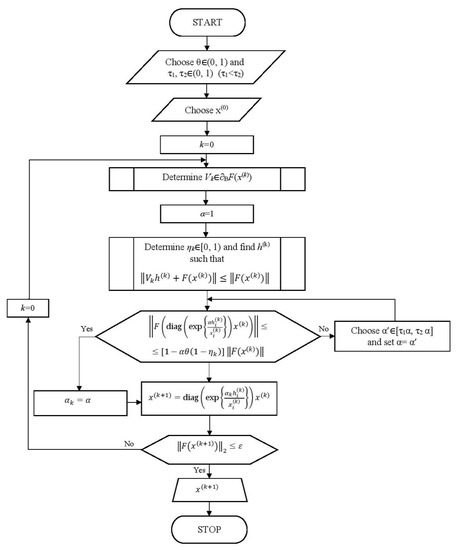
Figure 1. Flowchart for Algorithm 1.

In all examples, $x^{\left(0\right)}$ is the starting approximation, and $N_{IEM}$ is the number of iterations performed by Algorithm 1. For comparison of the efficiency of the new method, we also show the results obtained in tests by the inexact generalized Newton (IGM) method presented in [20] ($N_{IGM}$), which also has superlinear convergence.

Example 1.

As the first (double) test problem, we chose the usual Equation (1) with two different nonsmooth functions:

$$\begin{array}{ccc}{F}_1\left(x\right)\hfill & =\hfill & 0.2x\left|x-1\right|+e^{x-0.5}-1.05,\hfill \\ F_2\left(x\right)\hfill & =\hfill & \left[\begin{array}{c}\left|x_1\right|+{(x_2-1)}^2-1\\ {(x_1-1)}^2+\left|x_2\right|-1\end{array}\right]\hfill \end{array}$$

The equation with function $F_1$ has one solution $x^{\ast }=0.5$, while the equation with function $F_2$ has two solutions: $(0,0)$ and $(1,1)$. Both equations have one nondifferentiability point each: $x=1$ for $F_1$ and $x=(0,0)$ for $F_2$.

Both functions $F_1$ and $F_2$ are locally Lipschitz at their solution points. $F_1$ is $C^1$ at $x^{\ast }$ because

$$F_1^{\prime }\left(x\right)=\left\{\begin{array}{c}-0.2(x-2)+e^{x-0.5} \mathrm{for} x<1,\\ 0.2(x-2)+e^{x-0.5} \mathrm{for} x>1,\end{array}\right.$$

Therefore, $F_1$ is also semismooth at $x^{\ast }$. In turn, Qi and Sun proved in [14] that the function is semismooth at some point if and only if all of its component functions are semismooth at this point. And the component functions of $F_2$ are semismooth as the sum of the semismooth functions (the local Lipschitz continuities of the absolute value function and quadratic function are easy to check). Moreover, the Bouligand subdifferential of $F_1$ at $(0,0)$ has the form

$${\partial }_{B}F((0,0)=\left\{\left[\begin{array}{cc}-1& -2\\ -2& -1\end{array}\right],\left[\begin{array}{cc}-1& -2\\ -2& 1\end{array}\right],\left[\begin{array}{cc}1& -2\\ -2& -1\end{array}\right],\left[\begin{array}{cc}1& -2\\ -2& 1\end{array}\right]\right\}.$$

The equations can be solved by Algorithm 1. The only point of nondifferentiability of the function $F_1$ is not a solution, and function $F_2$ satisfies Assumption 1 (it follows from Remark 3(i)) and is BD-regular at $x^{\ast }=(0,0)$. The exemplary results are shown in Table 1 and Table 2.

Table 1. The numerical results obtained for the equation with function $F_1$ from Example 1.

${\mathit{x}}^{\left(0\right)}$	${\mathit{N}}_{\mathit{I}\mathit{E}\mathit{M}}$	${\mathit{N}}_{\mathit{I}\mathit{G}\mathit{M}}$
$-1$	34	41
0.1	16	19
0.3	5	6
0.7	5	6
1	7	9
5	13	16
10	18	20
50	69	74
100	132	147

Table 2. The numerical results obtained for the equation with function $F_2$ from Example 1 ($x^{\ast }$ indicates to which solution the sequence converged.).

${\mathit{x}}^{\left(0\right)}$	${\mathit{N}}_{\mathit{I}\mathit{E}\mathit{M}}$	${\mathit{N}}_{\mathit{I}\mathit{G}\mathit{M}}$	${\mathit{x}}^{\ast }$
($-100,-100$)	33	35	(0,0)
($-10,-10$)	28	27	(0,0)
($-10,-5$)	34	38	(0,0)
($-5,-5$)	21	26	(0,0)
($-1,-1$)	15	17	(0,0)
($-0.5,-0.5$)	13	15	(0,0)
(0.5,0.5)	17	19	(1,1)
(5,5)	8	10	(1,1)
(5,10)	9	12	(1,1)
(10,10)	10	14	(1,1)
(100,100)	16	19	(1,1)
($-1$,0.5)	27	31	(0,0)
(2,$-0.5$)	34	39	(1,1)

Example 2.

The second test problem was Equation (1) with the function $F:R^n\to R^n$ (used among the others in [4]), defined by

$$f_i\left(x\right)=\left\{\begin{array}{c}{c}_1{g}_i\left(x\right) \mathrm{for} g_i\left(x\right)\ge 0,\\ c_2{g}_i\left(x\right) \mathrm{for} g_i\left(x\right)\le 0,\end{array}\right.$$

with

$$g_i\left(x\right)=i-\sum _{j=1}^i\left\{cos(x_j-1)+j\left[1-cos(x_j-1)\right]-sin(x_j-1)\right\}.$$

Obviously, if $c_1=c_2$, then function F is differentiable. Therefore, the value $\left|c_1-c_2\right|$ may be treated as the degree of nondifferentiability of function F [22]. Equation (1) has an infinite number of solutions ${(1+2k_1\pi ,\dots ,1+2k_n\pi )}^T$, where $k_1,\dots ,k_n\in$$Z$ are arbitrary. First, the starting approximation was $\left(0,\dots ,0\right)$. We used Algorithm 1 to solve one series of smooth problems (with $c_1=c_2=1$) and three series of nonsmooth problems with various parameters $c_1=-c_2=1,10,100$.

Function F is semismooth as a composite of semismooth functions (as mentioned in Example 1), and all functions $f_i$ are semismooth as piecewise smooth functions (see [13]).

In the smooth case, Algorithm 1 (IEM) stopped after six iterations, while Algorithm IGM generated seven successive approximations. The most interesting results we selected are presented in Table 3.

Table 3. The numerical results obtained for the equation from Example 2 (n is the number of component functions.).

	${\mathit{c}}_1=-{\mathit{c}}_2=1$		${\mathit{c}}_1=-{\mathit{c}}_2=10$		${\mathit{c}}_1=-{\mathit{c}}_2=100$
$\mathit{n}$	${\mathit{N}}_{\mathit{I}\mathit{E}\mathit{M}}$	${\mathit{N}}_{\mathit{I}\mathit{G}\mathit{M}}$	${\mathit{N}}_{\mathit{I}\mathit{E}\mathit{M}}$	${\mathit{N}}_{\mathit{I}\mathit{G}\mathit{M}}$	${\mathit{N}}_{\mathit{I}\mathit{E}\mathit{M}}$	${\mathit{N}}_{\mathit{I}\mathit{G}\mathit{M}}$
2	5	6	5	6	5	6
3	5	6	5	7	6	7
4	6	7	7	8	8	8
5	6	8	7	8	8	9
8	8	10	9	9	9	10
10	9	10	9	10	10	11
12	10	11	10	11	11	11
15	19	21	23	27	25	30
20	17	19	19	23	18	21

In these tests, we noticed that the choice of starting point did not affect the number of iterations very much when Algorithm 1 generated a convergent sequence. Therefore, we omitted the results for other starting points. The number of iterations was actually very similar for a small number of variables. However, Algorithm 1 showed its advantage for larger problems (i.e., when a system of nonlinear equations has at least a dozen unknowns).

Example 3.

The last test problem was the Walrasian production–price problem [23] with the demand function ξ defined in the following form:

$${\xi }_j\left(\pi \right)=\sum _{i=1}^l\frac{a_{ij}{\varphi }_i\left(\pi \right)}{{\pi }_j^{b_i}},j=1,\dots ,m.$$

Here, $\pi \in R^m$ is the price vector, $a_{ij}$ measures the i-th consumer’s intensity of demand for commodity j, and $b_i$ is the i-th consumer’s elasticity of substitution for $i=1,\dots ,l$. Furthermore, the following

$${\varphi }_i\left(\pi \right)=\frac{{\sum }_{k=1}^m{\pi }_k{\omega }_{ik}}{{\sum }_{k=1}^m{a}_{ik}{\pi }_k^{1-b_i}}$$

is a function of the price chosen in such way to satisfy the budget constraint for each unit. Let $B\in R^{m\times n}$ denote the technology, $w\in R^m$ denote the total endowment of the economy prior to production and $y\in R^n$ denote the production plan.

Then, the Walrasian model can be written as the nonlinear complementarity problem (NCP) in the form

$$\min \left(g\right(x),f(x\left)\right)=0$$

with the following functions:

$$\begin{array}{c}\hfill g\left(\pi ,y\right)=\left[\begin{array}{c}\pi \\ y\end{array}\right] \mathrm{and} f\left(\pi ,y\right)=\left[\begin{array}{c}\omega -\xi \left(\pi \right)+By\\ -B^T\pi \end{array}\right],\end{array}$$

where the operator “min” denotes the component-wise minimum of the vectors.

Function $F\left(x\right)=\min \left(g\right(x),f(x\left)\right)$ is locally Lipschitzian, semismooth and BD-regular, so we can use Algorithm 1 to solve nonsmooth Equation (1).

An approximate solution of such a problem (NCP) with $m=6$, $n=8$ and $l=5$ is

$$\tilde{x}=\left(0.220,0.251,0.161,0.055,0.106,0.207,0.463,0,3.940,0.006,0,0,0.438,0\right).$$

We solved this problem using the inexact exponential method with various starting approximations from the neighborhood of $\tilde{x}$ in the form

$$x^{\left(0\right)}=\tilde{x}+a_1\dot{e}+a_2\ddot{e},$$

where $\dot{e}=\left(1,1,1,1,1,1,0,\dots ,0\right)\in R^{14}$ and $\ddot{e}=\left(0,0,0,0,0,0,1,\dots ,1\right)\in R^{14}$. The exemplary results are shown in Table 4.

Table 4. The numerical results obtained for the Walrasian production–price problem from Example 3 with various parameters $a_1$ and $a_2$.

${\mathit{a}}_1$	0.02	0.2	0.0	0.5	2.0
$a_2$	0.02	0.0	0.2	0.5	2.0
$N_{IEM}$	20	11	79	63	224
$N_{IGM}$	22	12	97	73	253

The Broyden-like method (from [24]) generated somewhat comparable results, which was not surprising since all these methods have the same order of convergence. The number of iterations was equal to 27, 9, −, 66 and 263 for the same initial points as in Table 4. In this test problem, the convergence significantly depended on the location of the starting point (parameters $a_1$ and $a_2$). Here, Algorithm 1 showed its advantage for initial points further from the solution.

5. Conclusions

We have proposed a new inexact exponential method for solving systems of nonsmooth equations (Equation (1)). We proved that the presented method has global and superlinear convergence under some mild assumptions when function F is locally Lipschitz continuous. In practice, Algorithm 1 (IEM) was significantly faster than the usual inexact generalized Newton (IGM) method. The used globalization technique turned out to be an effective approach to improve convergence behavior. The results of the numerical tests confirmed that the new inexact exponential method can be used to effectively solve miscellaneous nonsmooth problems such as nonsmooth equations, nonlinear complementarity problems or equlibrium problems.

References

- Pang, J.; Qi, L. Nonsmooth equations: Motivation and algorithms. SIAM J. Optim. 1993, 3, 443–465. [Google Scholar] [CrossRef]
- Chen, J.; Li, W. On new exponential quadratically convergent iterative formulae. Appl. Math. Comput. 2006, 180, 242–246. [Google Scholar] [CrossRef]
- Śmietański, M.J. On a new exponential iterative method for solving nonsmooth equations. Numer. Linear Algebra Appl. 2019, 25, e2255. [Google Scholar] [CrossRef]
- Martínez, J.M.; Qi, L. Inexact Newton method for solving nonsmooth equations. J. Comput. Appl. Math. 1995, 60, 127–145. [Google Scholar] [CrossRef]
- Pu, D.; Tian, W. Globally convergent inexact generalized Newton’s methods for nonsmooth equations. J. Comput. Appl. Math. 2002, 138, 37–49. [Google Scholar] [CrossRef]
- Bonettini, S.; Tinti, F. A nonmonotone semismooth inexact Newton method. Optim. Meth. Soft. 2007, 22, 637–657. [Google Scholar] [CrossRef][Green Version]
- Śmietański, M.J. Inexact quasi-Newton global convergent method for solving constrained nonsmooth equations. Int. J. Comput. Math. 2007, 84, 1157–1170. [Google Scholar] [CrossRef]
- Kahya, E. A class of exponential quadratically convergent iterative formulae for unconstrained optimization. Appl. Math. Comp. 2007, 186, 1010–1017. [Google Scholar] [CrossRef]
- Clarke, F.H. Optimization and Nonsmooth Analysis; SIAM: Philadelphia, PA, USA, 1990. [Google Scholar]
- Qi, L. C-Differential Operators, C-Differentiability and Generalized Newton Methods; Applied Mathematics Report AMR 96/5; University of New South Wales: Sydney, Australia, 1996. [Google Scholar]
- Sun, D.; Han, J. Newton and quasi-Newton methods for a class of nonsmooth equations and related problems. SIAM J. Optim. 1997, 7, 463–480. [Google Scholar] [CrossRef]
- Gao, Y. Newton methods for solving nonsmooth equations via a new subdifferential. Math. Meth. Oper. Res. 2001, 54, 239–257. [Google Scholar] [CrossRef]
- Mifflin, R. Semismooth and semiconvex functions in constrained optimization. SIAM J. Control Optim. 1977, 15, 959–972. [Google Scholar] [CrossRef]
- Qi, L.; Sun, J. A nonsmooth version of Newton’s method. Math. Program. 1993, 58, 353–367. [Google Scholar] [CrossRef]
- Qi, L. Convergence analysis of some algorithms for solving nonsmooth equations. Math. Oper. Res. 1993, 18, 227–244. [Google Scholar] [CrossRef]
- Potra, F.A.; Qi, L.; Sun, D. Secant methods for semismooth equations. Numer. Math. 1998, 80, 305–324. [Google Scholar] [CrossRef]
- Birgin, E.; Krejić, N.; Martínez, J.M. Globally convergent inexact quasi-Newton methods for solving nonlinear systems. Numer. Algorithms 2003, 32, 249–260. [Google Scholar] [CrossRef]
- An, H.; Mo, Z.; Liu, X. A choice of forcing terms in inexact Newton method. J. Comput. Appl. Math. 2007, 200, 47–60. [Google Scholar] [CrossRef]
- Song, Y.; Gowda, M.S.; Ravindran, G. On the characterizations of P- and P0-properties in nonsmooth functions. Math. Oper. Res. 2000, 25, 400–408. [Google Scholar] [CrossRef]
- Śmietański, M.J. Some superlinearly convergent inexact quasi-Newton method for solving nonsmooth equations. Optim. Meth. Soft. 2012, 27, 405–417. [Google Scholar] [CrossRef]
- Yamashita, N.; Fukushima, M. On the rate of convergence of the Levenberg-Marquardt method. Computing 2001, 15, 237–249. [Google Scholar]
- Spedicato, E. Computational Experience with Quasi-Newton Algorithms for Minimization Problems of Moderately Large Size; Report CISE-N-175; Centro Informazioni Studi Esperienze: Milan, Italy, 1 October 1975. [Google Scholar]
- Scarf, H. The Computation of Economic Equilibria; Yale University Press: New Haven, CT, USA, 1973. [Google Scholar]
- Chen, X.; Qi, L. A parametrized Newton method and a quasi-Newton method for nonsmooth equations. Comput. Optim. Appl. 1994, 3, 157–179. [Google Scholar] [CrossRef]
Disclaimer/Publisher’s Note: The statements, opinions and data contained in all publications are solely those of the individual author(s) and contributor(s) and not of MDPI and/or the editor(s). MDPI and/or the editor(s) disclaim responsibility for any injury to people or property resulting from any ideas, methods, instructions or products referred to in the content. |
© 2023 by the author. Licensee MDPI, Basel, Switzerland. This article is an open access article distributed under the terms and conditions of the Creative Commons Attribution (CC BY) license (https://creativecommons.org/licenses/by/4.0/).