Estimating the Frequencies of Maximal Theta-Gamma Coupling in EEG during the N-Back Task: Sensitivity to Methodology and Temporal Instability

Abstract

Phase-amplitude coupling (PAC) of theta and gamma rhythms of the brain has been observed in animals and humans, with evidence of its involvement in cognitive functions and brain disorders. This motivates finding individual frequencies of maximal theta-gamma coupling (TGC) and using them to adjust brain stimulation. This use implies the stability of the frequencies at least during the investigation, which has not been sufficiently studied. Meanwhile, there is a range of available algorithms for PAC estimation in the literature. We explored several options at different steps of the calculation, applying the resulting algorithms to the EEG data of 16 healthy subjects performing the n-back working memory task, as well as a benchmark recording with previously reported strong PAC. By comparing the results for the two halves of each session, we estimated reproducibility at a time scale of a few minutes. For the benchmark data, the results were largely similar between the algorithms and stable over time. However, for the EEG, the results depended substantially on the algorithm, while also showing poor reproducibility, challenging the validity of using them for personalizing brain stimulation. Further research is needed on the PAC estimation algorithms, cognitive tasks, and other aspects to reliably determine and effectively use TGC parameters in neuromodulation.

1. Introduction

A prominent feature of brain signals recorded extracellularly at high temporal resolutions is the existence of rhythmic oscillations in several frequency bands that span from approximately 0.05 Hz to 500 Hz [1]. Extensive research in animals and humans has provided mounting evidence of the involvement of these rhythms in various brain functions, from sensorimotor to cognitive ones [1,2], as well as their alterations in neurological and psychiatric disorders [3,4].

Brain oscillations exhibit a number of spatiotemporal relationships, including correlations of rhythms at different frequencies (cross-frequency coupling, CFC). One type of CFC is phase-amplitude coupling (PAC), i.e., the modulation of the amplitude of a high-frequency rhythm by the phase of a low-frequency oscillation. The earliest observations of PAC were in the rat hippocampus [5] between the phase of theta waves (5–10 Hz) and the amplitude of gamma activity (40–150 Hz), termed theta-gamma coupling (TGC). PAC was later reported between other frequency bands, in other animals and humans, in recordings by both invasive [6,7] and noninvasive [8] techniques.

PAC was found to be correlated with cognitive states and performance [9,10] and altered in a number of brain disorders [11,12]. This suggests that it may play an important role in the functioning of the brain. A prominent hypothesis about the role of PAC in working memory suggested in [13] is that each remembered item is encoded by the spatial pattern of a group of cells, and every such group synchronously fires in a different high-frequency subcycle of the low-frequency oscillation. This was supported by studies of grid cells in the entorhinal cortex [14,15]. The model suggested an explanation of the classic working memory capacity limit (span) of 7 ± 2 [16] as being determined by the number of gamma cycles within a theta cycle, although the evidence about this relationship has been mixed [17,18].

The implication of PAC in brain function motivates its use for informing neuromodulatory interventions, including non-invasive transcranial electrical and magnetic stimulation (TES and TMS) [1,19]. Recent studies have used individual frequencies of maximal TGC as parameters in protocols for transcranial alternating current stimulation (tACS) [20] or TMS [21]. This use implies that the determined frequencies of maximal coupling, at least to a certain approximation, constitute stable characteristics of each individual subject. However, there is insufficient data on the degree of session-to-session reliability of these parameters. One study [18] reported that the gamma frequencies of maximal coupling in two sessions had a (relatively low) Spearman correlation of 0.32, p = 0.03 (n = 44), while the theta frequencies were not correlated. This raises concerns about the possibility of reliable TGC peak frequency estimation. However, the data in the mentioned study were recorded in the resting state, and the situation may be different for measurements during cognitive tasks. Moreover, reliability may depend on the selection of data (electrodes and time periods) for analysis and the specific data processing algorithm employed.

Indeed, the methodology of PAC calculation from EEG signals in the literature is highly heterogeneous. The general procedure comprises several steps, including preprocessing, data selection, filtering the signals in the frequency ranges of interest, calculating a measure of PAC strength, and its normalization. In each of the steps, several options have been suggested and used in different studies. A number of methodological papers have compared some of the existing PAC calculation algorithms [22,23,24,25,26,27,28,29]. They mainly compared different modulation indices and, less often, the available approaches to filtering (wavelet transform with different numbers of cycles, band-pass filters, and the selection of their bandwidths). Importantly, the performance goal for a PAC calculation method was robust detection of coupling in the presence of noise and confounding factors, preferably from minimal data length, and with reasonable computation time. However, even a robust estimate of PAC will not necessarily be reproducible between measurements. Additionally, method performance was usually assessed using simulated data, which is important for isolating the impact of specific aspects of the signal, but may not reproduce the whole complexity of neural data.

Thus, the aim of our study was to estimate the trial-to-trial reliability of PAC patterns (comodulograms) and the frequencies of maximal coupling in the theta-gamma range. Several methods of PAC calculation were compared in these respects as applied to surface EEG recordings in a sample of healthy subjects performing the 3-back working memory task. In a preliminary analysis, we studied the performance of the algorithms on a signal with previously reported strong PAC from a publicly available rat local field potential (LFP) recording. The results could inform future uses of PAC analysis in the individualization of noninvasive brain modulation interventions in healthy subjects and patients with neurological and psychiatric disorders.

2. Materials and Methods

2.1. Benchmark LFP Data

To assess the performance of PAC calculation methods in a situation with previously reported strong coupling, we used a publicly available dataset [30] accompanying the scripts for PAC estimation deposited by the authors of the study [23] (time series named lfpHG). The data are from the study [31] investigating PAC in LFPs from the rat hippocampus during active waking and REM sleep. The duration is 300 s, with a sampling rate of 1000 Hz.

2.2. Participants

Sixteen healthy volunteers (9 women, mean age 29.6) were recruited for the study after signing an informed consent form. The study was approved by the local ethical committee of the Research Center of Neurology (protocol 3-7/22, 20 April 2022).

For the PAC reproducibility analysis, we selected a subsample of 14 subjects for which, after rejecting artifactual time periods, the remaining total time of epochs for PAC calculation (described below) in each of the two half-sessions was above 20 s.

2.3. 3-Back Task

The paradigm was implemented in the E-Prime 3.0 software (Psychology Software Tools, Sharpsburg, PA, USA). Each subject was presented with 3 series of 24 stimuli (6 target stimuli in each series). The stimuli were Latin consonant letters, each shown on the screen for 250 ms with an interval of 3000 ms between stimulus onsets. The subjects were instructed to press a button when the presented letter was the same as the one that appeared three letters before, in which case the current letter is called a target stimulus. Between the series of stimuli, there were breaks with the duration determined by the volunteer (around 10 s). Before the 3-back task, there were training sessions for similar 1-back and 2-back tasks.

2.4. EEG Recording

During the 3-back task, the subjects underwent EEG registration (64 electrodes placed according to the 10-10 system) using an actiCHamp Plus 64 (BP-100-2511) system (Brain Products GmbH, Gilching, Germany) synchronized with the paradigm by a Trigger Station system (BrainTrends, Rome, Italy). The initial reference was Cz, and the sampling rate was 1000 Hz.

2.5. EEG Preprocessing

Preprocessing and analysis of EEG data were carried out in the software package EEGLAB 2022.1 [32] and custom scripts in MATLAB R2022a (MathWorks, Natick, MA, USA). Channels with a high level of noise were removed, and the data were re-referenced to the common average. We applied a 1–80 Hz band-pass filter and a 49–51 Hz band-stop filter to reduce line noise (both performed in the EEGLAB graphical interface with default parameters, which calls the function pop_eegfiltnew implementing a delay-corrected (zero-phase) finite impulse response (FIR) filter). Time intervals with large artifacts from muscular activity or electrode motion were removed. Independent component analysis (ICA) was performed for the removal of non-neural components corresponding to eye blinks and saccadic movements, as well as persistent muscle activity.

We note that in the existing studies of PAC in EEG, there is some heterogeneity in preprocessing. For example, although many groups analyze data referenced to the common average [21,33,34,35,36], others use average mastoid reference [37,38].

2.6. Spectrum Calculation

We estimated the power spectral density (PSD) to assess the frequency content of EEG signals and the presence of theta peaks, which has been identified as a prerequisite for a meaningful interpretation of PAC, although checked in less than half of the papers reviewed in [25]. We used the EEGLAB function spectopo applying the Welch method, with a one-second-long Hamming window, 50% overlap, and oversampling by zero-padding to twice the window size.

2.7. TGC Computation

2.7.1. Steps of PAC Calculation and Variations in Them

After EEG preprocessing, the steps performed to estimate PAC are as follows:

• Selection of electrodes;
• Extraction of oscillations for phase and amplitude;
• Selection of epochs (time intervals) for PAC calculation (optional);
• Calculation of a PAC measure;
• Normalization of the PAC measure (optional);
• Averaging the PAC measure over subsets of the data (optional).

Following are descriptions of the available options in each step and our choices among them.

2.7.2. Selection of Electrodes

One way of computing PAC is within a channel, so that one electrode provides both the low-frequency signal for phase and the high-frequency signal for amplitude. This approach can be applied in a focused way to one or a few electrodes (e.g., two in [39]), or in a more exploratory way to many electrodes (19 in [40]). A combination of these approaches is an analysis of all the electrodes followed by averaging the PAC measure over a subset, such as the frontal electrodes in [12,37,38,41]. The focused approach is limited by the plausibility of the a priori hypothesis about the location of the relevant coupling, while the exploratory analysis may suffer from a power decrease due to multiple comparisons, depending on the research question.

Another option is computing PAC between different electrodes, one providing phase and the other defining amplitude. This has the methodological advantage of reducing the likelihood of the common driver effect, which prevents causal interpretation of the coupling [25]. This approach is also necessary if coupling between distant neuronal populations is being researched. In the existing studies of between-channel TGC, the theta phase was usually taken from frontal electrodes, while the gamma amplitude was extracted from parietal [33,34] or all channels [42]. In a more focused way, the study [21] used theta phase from Fz and gamma amplitude from Pz. We employ this last approach in all calculations except one, in which we use Fz for both theta and gamma (named ‘within channel’, further described below) to explore frontal within-channel PAC studied in several above-mentioned papers.

2.7.3. Extraction of Oscillations for Phase and Amplitude

Band-Pass Filters: Filter Type

One way of extracting the oscillatory components is band-pass filtering followed by the Hilbert transform. The filters applied usually have a zero phase shift to preserve the temporal relationship between phase and amplitude. At least three ways of constructing such filters have been used in PAC literature. The first one is the forward and backward (two-way) application of a Butterworth infinite impulse response (IIR) filter [21,26,43]. The second option is a two-way finite impulse response (FIR) filter as implemented in the EEGLAB function eegfilt [7,23,31,33,34,36,40,44,45]. Finally, the third approach is a forward application of a FIR filter followed by shifting the data by the filter’s group delay, as implemented in the function pop_eegfiltnew from the firfilt plugin for EEGLAB [28,35,46,47]. The orders and transition bands of the filters can be chosen in different ways, but they are usually kept at default values in the mentioned functions. In some papers, the exact filter type is not mentioned [39], or a partial description is provided, such as ‘second-order zero-phase shift’ in [37], with later papers [12,38] referencing this one regarding the methods.

The EEGLAB package switched its default filter from pop_eegfilt (calling eegfilt) to pop_eegfiltnew, and its website states that “the heuristic for automatically determining the filter length in the legacy basic FIR filter (pop_eegfilt) was inappropriate (possibly causing suboptimal filtering or unexpected filter effects)”. At the same time, the number of papers using eegfilt (including recent ones) cited above shows that it is probably still the most popular method. Thus, we used eegfilt (with default parameters) as a starting point (in the ‘basic’ method below), but also explored the Butterworth filter (MATLAB function butter with n = 2 and forward-backward application by function filtfilt) and pop_eegfiltnew (with default parameters).

It should be noted that our signals after preprocessing contain boundaries from artifactual time interval rejection. The function pop_eegfiltnew uses DC padding around any continuous time interval, which arguably creates smaller distortions at the edges than filtering across a boundary [48]. Thus, in the versions of the algorithm without buffer zones or without selecting epochs (described below), we used pop_eegfiltnew rather than the functions eegfilt or butter. In the versions with buffer zones, a boundary will be separated from the PAC calculation interval by at least the buffer zone length, and the distortions are unlikely to affect the PAC.

Band-Pass Filters: Band Definition

Another issue besides the filter type is the choice of the band. Some papers compute the coupling for two fixed frequency bands, such as the theta band of 4–7 Hz and gamma band of 30–50 Hz used in [12,37,38,41]. Other definitions of the gamma band include 30–40 Hz to avoid contamination with line noise in [35], 36–45 Hz in [40], 50–80 Hz in [33] and 50–70 in [34]. It is interesting to note that the last two studies (sharing three of the authors) used two almost mutually exclusive definitions of the theta band: 5–8 Hz and 3–5 Hz, respectively.

Rather than using fixed bands and obtaining one PAC value, an exploratory analysis can be performed, i.e., computing the coupling for a series of bands. A comodulogram can then be produced, which is a plot with band-center frequencies on the axes and the corresponding PAC measure depicted by color. The widths of the bands can be fixed, e.g., 4 Hz for phase and 20 Hz for amplitude [45], or, respectively, 1 and 4 Hz [7], 2 and 40 Hz [36], 4 and 10 Hz [23,31], 2 and 5 Hz [47], and 2 and 4 Hz [44]. It has been pointed out that if the bandwidth for amplitude is smaller than twice the modulating (phase) frequency, then it does not include the side peaks produced by the modulation, and PAC cannot be detected even if it is present [24,25]. This raises concern about the correctness of the analysis in the papers using narrow bands for amplitude. At the same time, as explained in [24], in the eegfilt function, the transition bands scale with increasing frequency. This results in a higher total bandwidth of the filter than intended and possibly enables such a filter to extract the modulated signal. Overall, the question of minimally sufficient bandwidth for amplitude for different filter types needs further clarification.

In addition to using fixed bandwidths, there is an adaptive approach aimed at obtaining the best frequency resolution while satisfying the above-mentioned side-peak condition. Thus, in [21], the bandwidth for amplitude was set to 2 f_p + 4 Hz, where f_p is the phase band-center frequency, while in [28], it was set to 2 f_p. A similar but distinct approach is to set the bandwidth for amplitude to twice the maximum considered phase frequency, as is set by default in the package pactools (in the Python programming language) described in [49].

In this study, we used as a starting point (‘basic’ method below) the bandwidths of 4 and 20 Hz for phase and amplitude, considering that they satisfy the side-peak condition for TGC and were used in the scripts deposited by A. Tort et al., producing strong PAC in the benchmark LFP data. We also tested the adaptive bandwidth approach from [21] (method ‘Butterworth adaptive’ below).

For band center frequencies, we adopted the settings from [21], calculating the comodulograms in the 3–9 Hz range for phase and the 20–70 Hz range for amplitude, and then selecting the frequencies of maximal coupling within the window of 4–8 Hz for phase and 30–60 Hz for amplitude. The initial calculation of the coupling over the larger windows allowed us to check whether the maximum in our window was indeed a local maximum of PAC or lied on a slope from a peak located outside this window. In this latter case, the comodulogram can be said to be dominated by the coupling of other rhythms that obscure the TGC.

Wavelet Transform

An alternative to band-pass filtering and the Hilbert transform is the use of a complex Morlet wavelet transform. The equivalent to the question of bandwidth choice here is the selection of the number of cycles in the wavelets [50]. PAC studies have employed wavelets for both phase and amplitude with 5 cycles [51,52], or 7 cycles [24]. When this number is fixed for all the wavelet frequencies, the time resolution of the transformation increases with frequency, while the frequency resolution decreases [50,53]. To improve the frequency resolution at the cost of some decrease in the temporal resolution at higher frequencies, the number of wavelet cycles can be set to increase with the frequency [50]. This approach has been implemented in the wavelet-based time-frequency decomposition in the EEGLAB function newtimef, which is used in the PAC calculation plugin PACTools for EEGLAB [54]. The numbers of cycles in this plugin are controlled by the variables ‘cycles’ for phase and ‘cycles2’ for amplitude, set by default to [3 0.5] and [10 0.5]. This means that, for phase, at the lowest frequency the number of cycles is 3, and at the highest frequency it is such that the wavelet standard deviation in the time domain is 0.5 of its value for the lowest frequency, and similarly for amplitude, starting from 10 cycles.

In our calculations, one method variant had fixed numbers of cycles. For phase, we used 6 cycles, which we chose empirically as the smallest number producing few phase slips and reverses, which are a sign of the filter for phase being too wide [25]. For amplitude, we used 4 cycles to obtain approximately the smallest standard deviation in the frequency domain that satisfies the side-peak condition. In an alternative method, we used the adaptive cycle numbers from PACTools. The center frequencies for the wavelets were selected in the same way as for band-pass filters (previous section).

2.7.4. Selection of Epochs for PAC Calculation

In studies with behavioral tasks, the signal often contains evoked responses to visual stimuli and event-related potentials due to button presses. Additionally, different periods of the task may be associated with different cognitive states. Thus, in this context, PAC is usually calculated at certain time intervals (epochs) defined by events such as stimulus onsets. For example, in [43], the epochs were 1000 ms delay periods between the encoding and test stimuli, and in [40], they were the intervals at 0–2000 ms before the stimuli in the 2-back task. A common consideration in selecting the epochs is excluding the visual-evoked potentials (VEP) [21,33]. However, some studies do not follow this recommendation, e.g., in [34], PAC was calculated during the 100–1500 ms period from the start of the visual stimulus presentation, which lasted 2 s. Moreover, an essentially opposite approach was adopted in the studies [12,37,38], where each epoch for PAC calculation started with the stimulus onset and ended at the time of response. The authors concatenated several such epochs to obtain a signal of 5000 ± 150 ms length, which in the 3-back task required on average 8.23 epochs in [37]. Thus, the mean duration of an epoch was ~600 ms, of which more than half probably contained a substantial VEP. At the same time, this approach largely excludes the evoked potential from the button press (except for its spread due to temporal smoothing by low-frequency filters), while this potential likely contaminates the later periods used in other studies of the n-back task.

In our ‘basic’ method, we considered ‘VEP-free’ intervals lasting from 500 ms from stimulus onset (=250 ms from its offset) until 3000 ms when the next stimulus appeared and selected only the intervals without boundaries produced by artifactual time interval rejection. However, an often overlooked fact is that a filter creates temporal smoothing [50] and will spread the VEP into the adjacent time periods. Consequently, to avoid VEP influence, the contaminated portions must be discarded, and so we removed buffer zones at each end of a ‘VEP-free’ interval (Figure 1). The length of the buffer zones was chosen to be three periods of the lowest considered theta frequency of 4 Hz, i.e., 750 ms. Thus, PAC was calculated over 1000-ms epochs at the latencies 1250–2250 ms from stimulus onset.

In view of the substantial reduction of the total signal length by the buffer zones, we also considered an alternative method without them, as well as a variant with PAC calculation over the entire session, without selecting any epochs.

In regard to the ‘VEP-free’ intervals, we decided to avoid the term ‘maintenance periods’, as they are sometimes called [21,40], because in the 3-back task, at least three stimuli need to be maintained in memory at all times, including the periods of stimulus presentation, and thus, apart from the beginning and end of a stimulus series, there are no ‘pure encoding’ or ‘pure retrieval’ periods.

The benchmark LFP data contained no events, so in our analysis, we treated them as continuous, i.e., without selecting epochs, in all algorithm variants but one. In this last variant (‘simulated epochs’), we extracted epochs with the same timing as in one of the participants performing the 3-back task (after shortening the LFP data to match the length of the cleaned EEG for this subject, i.e., 224 s). This was carried out to explore the influence of epoching on PAC reliability, which could occur due to the reduction of the total data length as well as a possible specific interaction of the temporal structure of the epochs with brain rhythms. The total time of the selected epochs was 33 and 27 s in the two half-sessions in this calculation.

2.7.5. Calculation of a PAC Measure

The existing PAC measures have been described and compared in a number of papers [23,27,29]. We focused on two often-used parameters: the Kullback–Leibler modulation index (KL-MI) [23,37,43] and the mean vector length modulation index (MVL-MI) [7,26,39]. The MVL-MI in its raw (unnormalized) form scales linearly with the high-frequency amplitude. Thus, to measure the modulation independently from the high-frequency power, this index is usually normalized by either dividing by the root-mean-square amplitude [55] or using surrogates [7,26]. We adopted the second approach (described below). The KL-MI is sometimes normalized using surrogates [24,27,44] and sometimes not [23,35,36]. We explored both options.

2.7.6. Normalization of the PAC Measure

Normalization of PAC measures using surrogates involves generating artificial signals retaining most of the characteristics of the measured data, but with broken temporal relationships between the phase and amplitude [24]. The PAC measure for the actual signals is then normalized by subtracting the mean and dividing by the standard deviation of its values for the surrogate signals. This can be used to (1) remove the dependence of a PAC measure on the magnitude of the amplitude signal, (2) make the resulting measure comparable between different contexts, and (3) test the statistical significance of the coupling [50].

We generated surrogate signals by splitting the amplitude time series at an arbitrary point and swapping the two resulting segments (‘split-swap’ surrogates below), which is more appropriate than some alternative methods such as random permutation [25]. As explored in [24], when the minimum surrogate offset is smaller than 1 s, the normalized PAC measures tend to underestimate the coupling, presumably due to incomplete breaking of the temporal relationships between the phase and amplitude in some of the surrogates, leading to high PAC values for them. Thus, we pseudorandomly selected the splitting point between 0.1 and 0.9 of the whole signal length (setting adopted from the online scripts accompanying the book [50]). We used 200 surrogates for normalizing both the KL-MI and MVL-MI.

2.7.7. Averaging the PAC Measure over Subsets of the Data

In some studies, PAC measures are averaged over epochs or electrodes [40,41,52]. This can combine instances of coupling where the amplitude is increased at different values of the phase, and thus the resulting measure has a somewhat different meaning than a single PAC value computed from a number of epochs, which extracts only the PAC that is coherent between the epochs. We used the latter approach in this study (i.e., without averaging).

2.7.8. Algorithms Compared in This Study

In view of the above considerations, we selected nine algorithms of PAC computation for the benchmark LFP data, and a related but distinct set of nine algorithms for the 3-back EEG data.

Algorithms for Benchmark LFP Data

All coupling calculations for the benchmark data are within-channel.

All the algorithms from

Table 1. Parameters of the algorithms used to compute PAC in the benchmark LFP data.

Letter in Figures	Short Algorithm Name	Extraction of Oscillations	Width Parameters (Phase, Amplitude)	Epoch Selection	PAC Measure	Normalization
A	basic	two-way FIR filter (eegfilt)	4, 20 Hz	no	KL-MI	no
B	Butterworth	two-way Butterworth filter (butter, filtfilt)	4, 20 Hz	no	KL-MI	no
C	Butterworth adaptive	two-way Butterworth filter	4 Hz, 2 fp + 4 Hz	no	KL-MI	no
D	eegfiltnew	delay-corrected one-way FIR filter (pop_eegfiltnew)	4, 20 Hz	no	KL-MI	no
E	wavelet	Morlet wavelet transform	6, 4 cycles	no	KL-MI	no
F	wavelet adaptive	Morlet wavelet transform	adaptive cycles as in PACTools	no	KL-MI	no
G	normalized	two-way FIR filter	4, 20 Hz	no	KL-MI	200 ‘split-swap’ surrogates
H	MVL normalized	two-way FIR filter	4, 20 Hz	no	MVL-MI	200 ‘split-swap’ surrogates
I	simulated epochs	two-way FIR filter	4, 20 Hz	from 3-back 1250–2250 ms	KL-MI	no

were used to compute comodulograms for the benchmark data over the frequency ranges of 4–20 Hz with a 0.5 Hz step for phase and 20–200 Hz with a 5 Hz step for amplitude (slightly modified from the scripts deposited by A. Tort et al.). The maximum PAC was then selected in the windows of 4–10 Hz for phase and 30–200 Hz for amplitude.

Algorithms for the EEG Data with the 3-Back Task

In the following descriptions, ‘Fz-Pz’ means that theta phase was extracted from channel Fz, and gamma amplitude, from channel Pz.

All algorithms from

Table 2. Parameters of the algorithms used to compute PAC in the EEG data with the 3-back task.

Letter in Figures	Short Algorithm Name	Channels	Extraction of Oscillations	Width Parameters (Phase, Amplitude)	Epoch Selection (from Stimulus Onset)	PAC Measure	Normalization
A	basic	Fz-Pz	two-way FIR filter	4, 20 Hz	1250–2250 ms	KL-MI	no
B	Butterworth	Fz-Pz	two-way Butterworth filter	4, 20 Hz	1250–2250 ms	KL-MI	no
C	no buffer	Fz-Pz	delay-corrected one-way FIR filter	4, 20 Hz	500–3000 ms	KL-MI	no
D	eegfiltnew	Fz-Pz	delay-corrected one-way FIR filter	4, 20 Hz	1250–2250 ms	KL-MI	no
E	wavelet	Fz-Pz	Morlet wavelet transform	6, 4 cycles	1250–2250 ms	KL-MI	no
F	no epochs	Fz-Pz	delay-corrected one-way FIR filter	4, 20 Hz	no (all cleaned data)	KL-MI	no
G	normalized	Fz-Pz	two-way FIR filter	4, 20 Hz	1250–2250 ms	KL-MI	200 ‘split-swap’ surrogates
H	MVL normalized	Fz-Pz	two-way FIR filter	4, 20 Hz	1250–2250 ms	MVL-MI	200 ‘split-swap’ surrogates
I	within channel	Fz-Fz	two-way FIR filter	4, 20 Hz	1250–2250 ms	KL-MI	no

were used to compute the comodulograms for the n-back EEG data over the frequency ranges of 3–9 Hz with a 0.5 Hz step for phase and 20–70 Hz with a 5 Hz step for amplitude, with maximum PAC selected in the windows 4–8 and 30–60 Hz, respectively.

2.8. Reproducibility between Measurements: Characteristics and Statistical Tests

The general approach that we used in studying reproducibility consists in dividing an EEG (or LFP) session into two parts of equal length (half-sessions), computing the PAC measures for each of the half-sessions, and comparing the resulting comodulograms in terms of the overall similarity and the stability of the point of maximal theta-gamma coupling. The half-sessions can be considered as two smaller sessions performed one immediately after another. Such treatment of half-sessions as consecutive measurements has been used in EEG analysis in various contexts [56,57,58,59]. Repeatability between such measurements can be considered as the minimum requirement, indicating that the frequencies of maximal coupling are stable at least at the time scale of the session, and could be meaningfully used to guide neuromodulation performed shortly after the EEG measurement. Other applications may require stability at longer time scales.

To visualize the degree of general similarity of the comodulograms between the half-sessions, we used scatter plots where each point corresponds to a pair of frequency bands, and its coordinates are the values of PAC between these bands in the two half-sessions. In the case of exact reproducibility, these points will lie on the line “y = x”.

The similarity of two comodulograms was measured by the sample Spearman correlation coefficient (denoted by ρ) of all the PAC values in them. This metric has been used to compare comodulograms between methods in [60]. It must be stressed, however, that this context of using Spearman correlation differs from its usual application to a sample of realizations of independent, identically distributed (i.i.d.) random variables. In our situation, all PAC values in a comodulogram are computed from the same signals, and thus, generally speaking, they are dependent. This precludes running the usual statistical tests on ρ while not invalidating its use as a similarity measure.

To test whether the similarity of comodulograms between half-sessions differed on average from zero, we applied Wilcoxon’s signed-rank test to the values of ρ obtained in each subject. Here, in contrast to the previous discussion, the values are taken from different subjects and hence do form an i.i.d. sample.

The similarity between the comodulograms from half-sessions of a given individual can be due to specific reproducible features of the coupling pattern in this subject. However, it can also be unspecific, so that all the comodulograms calculated by a particular method are similar, regardless of whether they are obtained from the same or different subjects. To check this, we computed and plotted matrices of Spearman correlations between comodulograms from the first half-session of every subject with the second half-session of every other subject. In the event of the existence of reproducible and unique patterns in the comodulograms of each subject, these matrices should have large diagonal values (within-subject correlations) and smaller off-diagonal values (between-subject correlations).

The reproducibility between the half-sessions of the phase and amplitude frequencies of maximal TGC was characterized by two quantities: the mean absolute difference (change) and the intraclass correlation coefficients (ICC). The mean difference characterizes the absolute variability in Hz, while the ICC measures the reliability relative to the between-subject variance. We calculated ICC (C,1) in the terminology of [61] and tested the hypothesis “ICC = 0” using the MATLAB package “Intraclass Correlation Coefficient (ICC)” [62]. This test determines whether there is a significant subject effect on the frequencies (the p-values are actually the same as for the subject effect in a two-way ANOVA with factors: subject and half-session). Thus, this test shows if there are reliably inferred nonzero differences between mean frequencies for different subjects. This is important in the context of brain stimulation for the individualization procedures to be meaningful.

To compare the methods in terms of absolute variability of peak frequencies, we performed Friedman’s tests for the effect of the algorithm on the absolute frequency changes, followed by post-hoc tests using the Tukey–Kramer method.

To test for a possible effect of the half-session (due to fatigue, learning, or other causes), we performed Wilcoxon’s signed-rank tests on the peak frequencies from the two half-sessions for each PAC calculation method.

To illustrate the degree of reproducibility of the comodulograms, we included their plots and scatter plots between half-sessions for a single subject as an example. We selected this subject to have average peak variability. To this end, we calculated a composite measure of variability derived from both the phase and amplitude peak frequencies. This was performed by dividing the absolute frequency change by the length of the corresponding frequency range and averaging the resulting two values:

$$∆f_{composite}=\frac{1}{2}\left(\frac{∆f_p}{r_p}+\frac{∆f_a}{r_a}\right)$$

where $∆f_p$ is the absolute change between half-sessions of the phase frequency of maximum PAC, and similarly for $∆f_a$; $r_p$ and $r_a$ are the lengths of the theta and gamma frequency ranges (8 − 4 = 4 Hz and 60 − 30 = 30 Hz, respectively). Thus, this composite measure indicates by what fraction of the whole frequency interval the peak has shifted. The subject for illustrations was chosen to have the composite variability (averaged by all the algorithms) closest to the group median.

We also compared the algorithms in terms of the central tendency of the frequencies of maximal TGC to see if any of the methods produced consistently lower or higher peak frequencies. For this, we performed Friedman’s tests separately for the phase and amplitude peak frequencies, followed by post-hoc tests using the Tukey–Kramer method. This analysis was not concerned with reproducibility, and hence we performed it for comodulograms computed from whole sessions rather than half-sessions.

3. Results

3.1. Benchmark LFP Data

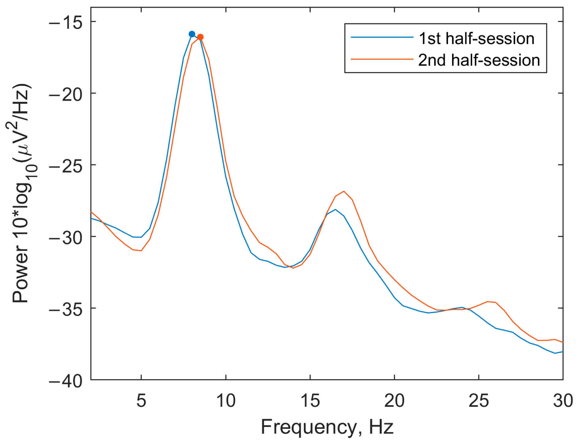
3.1.1. Spectra

The power spectral density for the benchmark LFP data from the rat hippocampus showed clear peaks at frequencies 8 and 8.5 Hz in the two half-sessions (Figure 2). Thus, there was a prominent theta-rhythm with a relatively stable peak frequency.

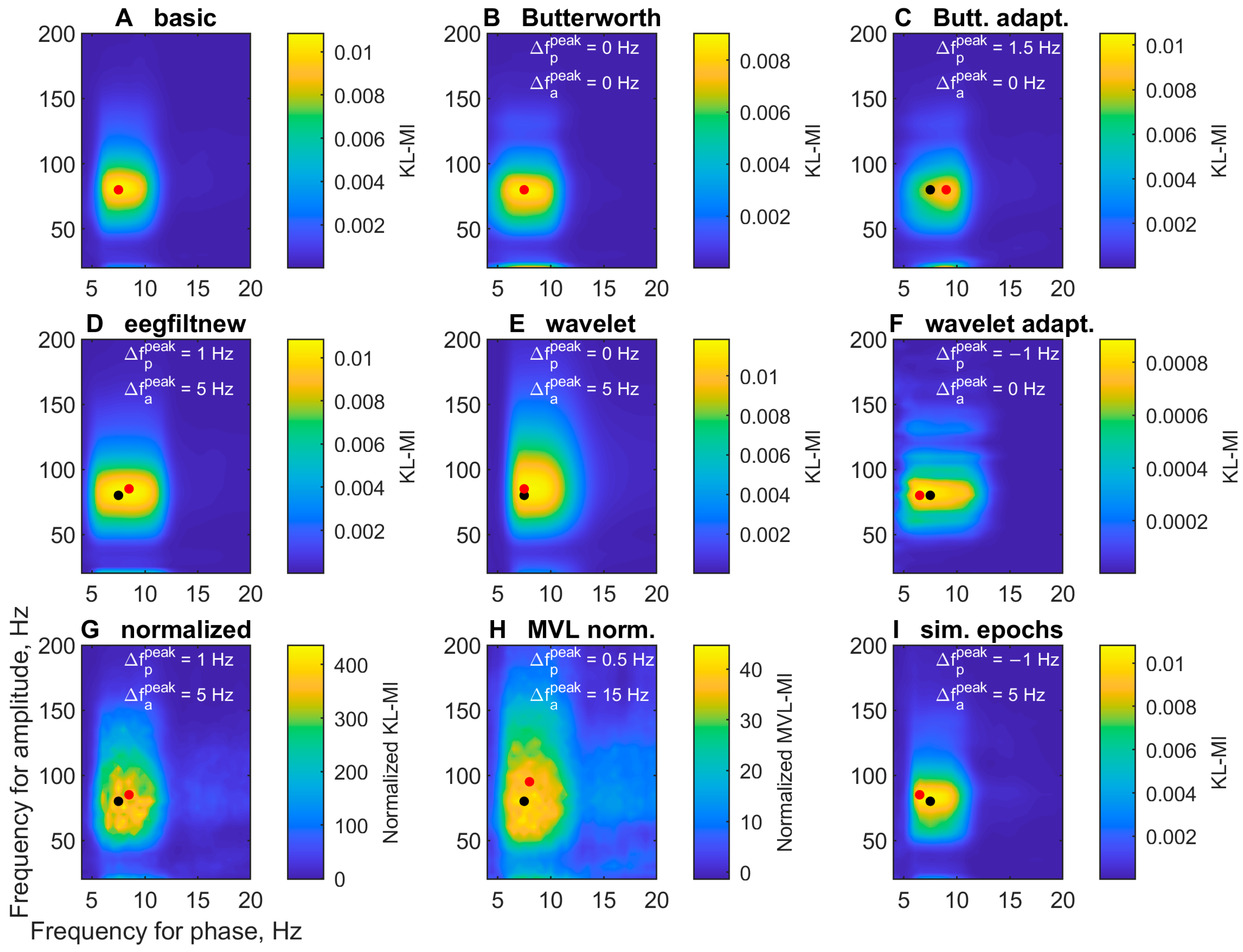
3.1.2. Comodulogram Dependence on the Algorithm

The comodulograms for the benchmark LFP data (calculated from the whole session) showed moderate dependence on the PAC calculation algorithm (Figure 3). They all had the same general appearance, each containing one bright peak at roughly similar locations. The peaks for the normalized indices appeared ‘patchy’ (possibly due to the randomness in surrogate signal generation). The differences in peak frequencies in methods B-I from the ones for the basic method (A) ranged from −1 to 1.5 Hz for phase and from 0 to 15 Hz for amplitude.

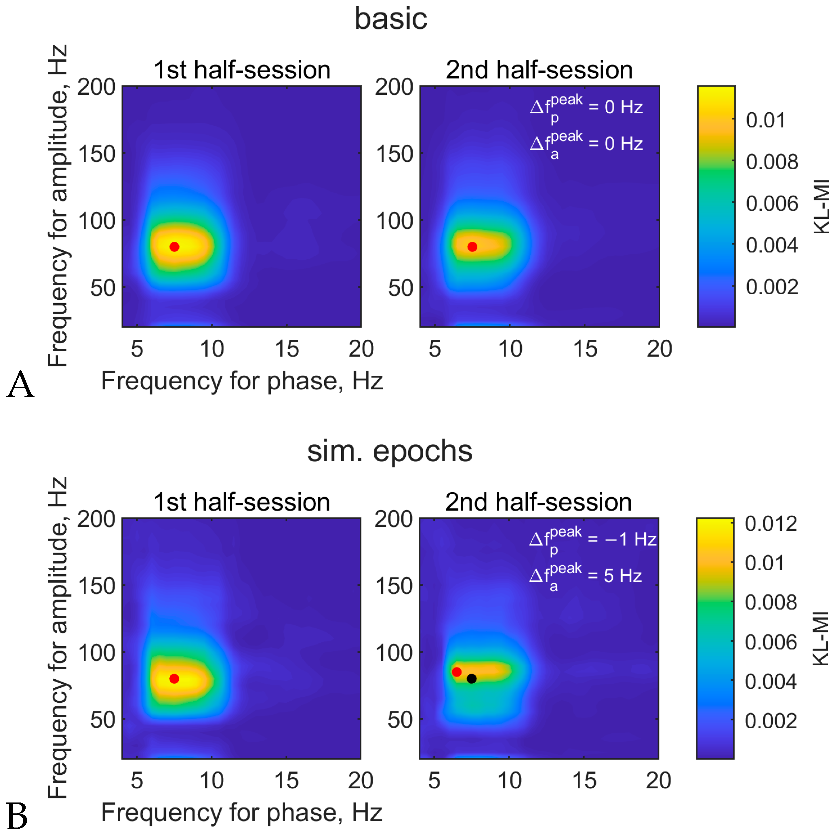
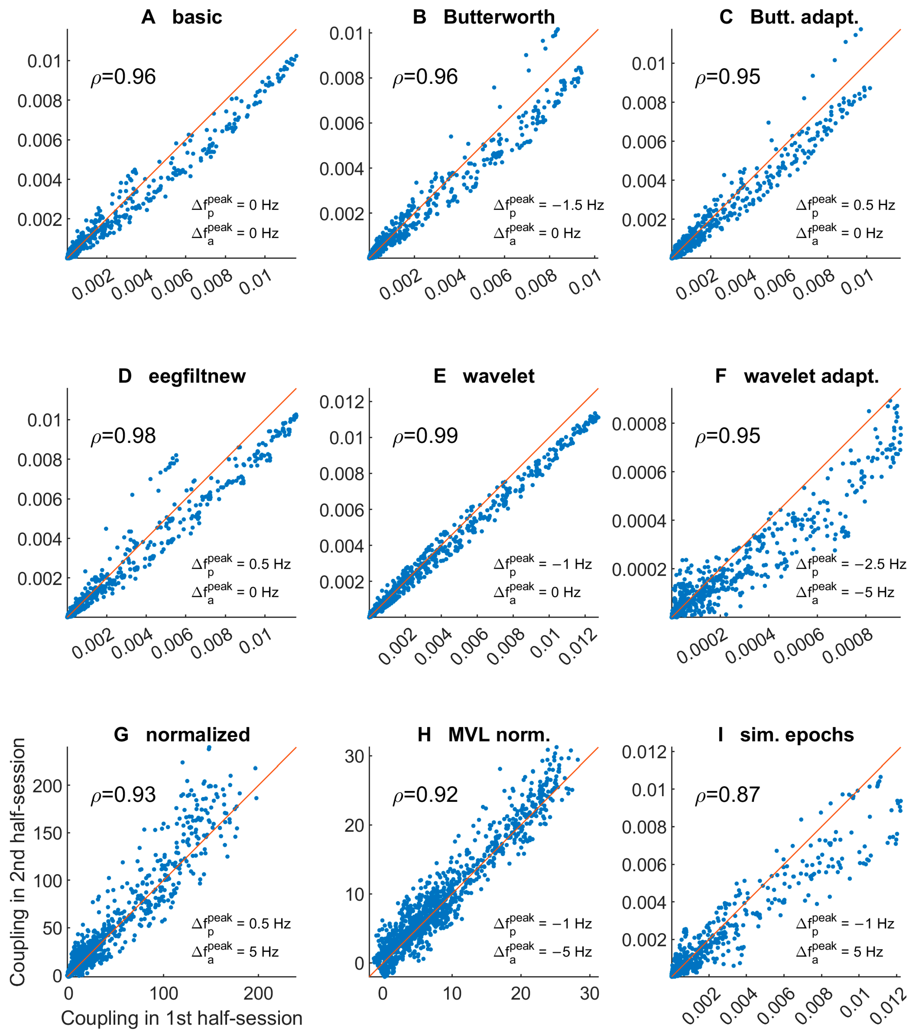
3.1.3. Comodulogram and Peak Variability between Half-Sessions

The comodulograms computed by the half-sessions (Figure 4) are generally similar to each other and to the ones from the whole session (Figure 3).

The scatter plots of PAC values from the two half-sessions (Figure 5) have points that are mostly concentrated near the line ‘y = x’, meaning that the couplings between the same frequency bands are similar in the two measurements. The Spearman correlation coefficients of the comodulograms range from 0.87 in the ‘simulated epochs’ method to 0.99 in the ‘wavelet’ algorithm. The peak frequency shifts between the half-sessions range from -2.5 to 0.5 Hz for phase and from −5 to 5 Hz for amplitude.

Overall, the coupling can be considered relatively stable, although the larger shifts of the phase frequency (−2.5 Hz in ‘wavelet adaptive’ and −1.5 Hz in ‘Butterworth’ algorithms) are noticeable compared to its value of approximately 8 Hz.

3.2. EEG during the 3-Back Task

3.2.1. Behavioral Statistics for the 3-Back Task

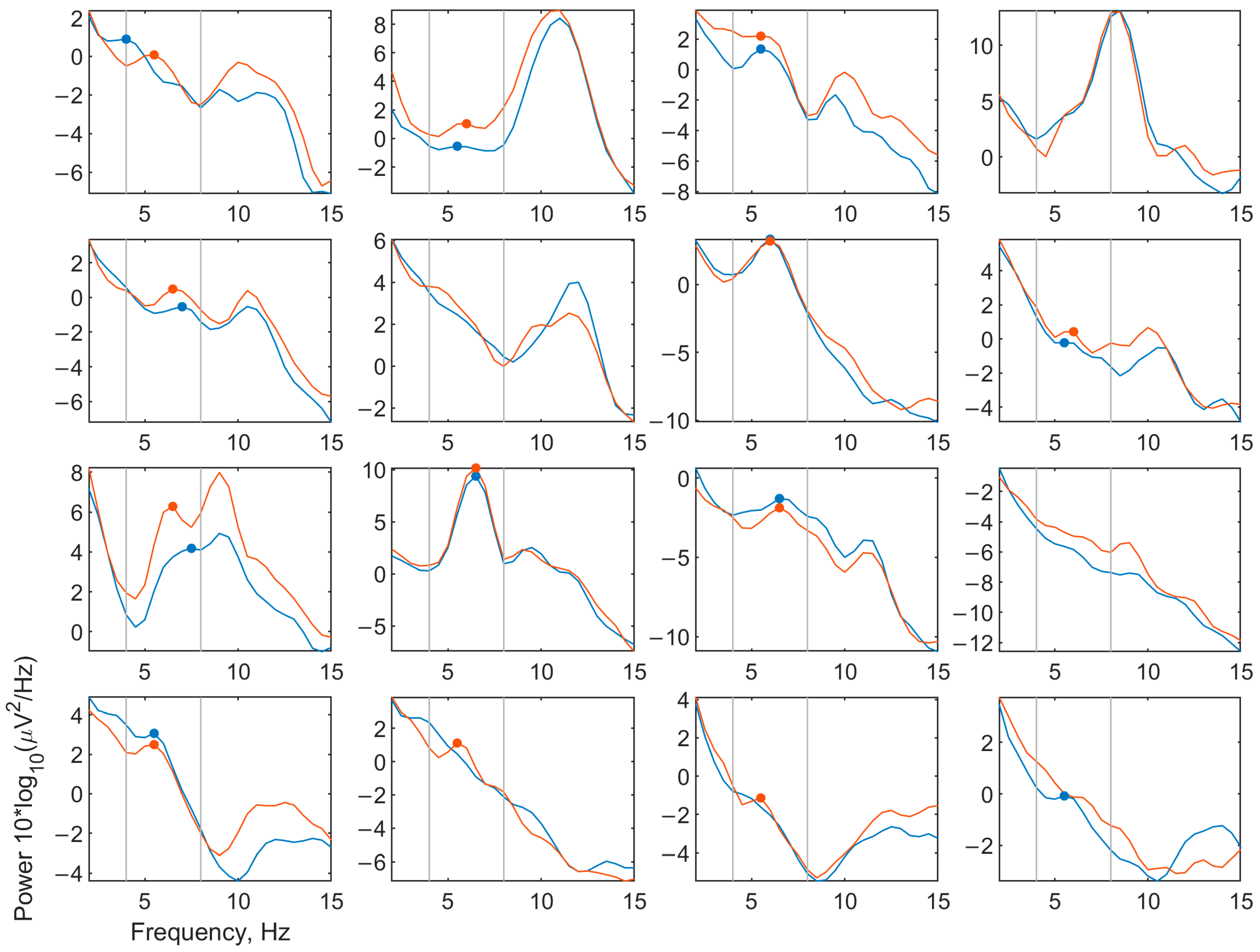
The fraction of correct responses to all stimuli ranged from 0.7 to 1, with a mean of 0.9, while the hit rate for target stimuli ranged from 0.5 to 1, with a mean of 0.76.

3.2.2. EEG Spectra

The power spectra (Figure 6) showed mixed results regarding theta peaks. Ten of the sixteen subjects had local maxima in the 4–8 Hz range in both half-sessions, some of these peaks being only slightly above the background. Three subjects had no local maxima in the considered range, while the remaining three had such a peak in only one of the half-sessions. The general shape of the spectra was similar between the half-sessions, while the details differed in some of the subjects, with theta peak shifts ranging from 0 to 1.5 Hz.

3.2.3. Length of EEG for PAC Calculation

During artifact rejection, some time intervals were removed from the EEG data. For the PAC reproducibility analysis, we selected a subsample of 14 subjects for which the remaining total time of epochs for PAC calculation (1250–2250 ms from stimulus onset) was above 20 s in each of the two half-sessions. In the selected subjects, this time ranged from 26 to 36 s (mean 31 s) in the first half-session and from 22 to 37 s (mean 31 s) in the second one. The total epoch time in the whole session ranged from 48 to 72 s (mean 62 s).

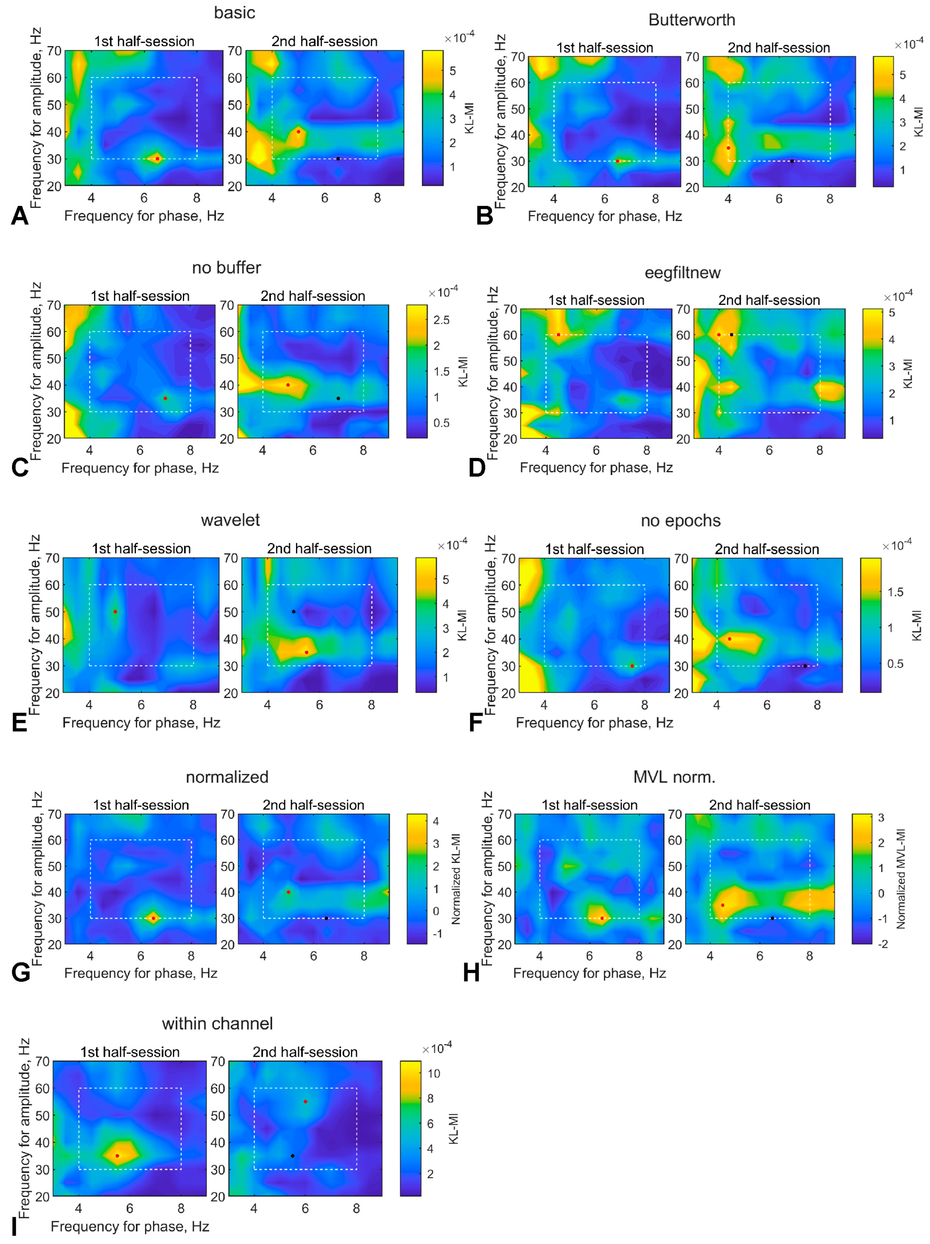
3.2.4. Comodulogram Dependence on the Algorithm

The group-mean phase frequencies of maximum coupling significantly differed between the algorithms (Friedman’s test, p = 0.002). Post-hoc tests (Tukey–Kramer) showed that the phase frequencies of maximum coupling were lower on average for the ‘basic’ and ‘Butterworth’ methods (which use the KL-MI) than for the ‘normalized MVL’ method (p = 0.01 and 0.02, medians of the differences −1.25 and −1.5 Hz), with no other significant differences. This is consistent with most peaks concentrating in the left parts of the plots (Section 3.2.6). No significant differences between the algorithms were found in the group-mean amplitude frequencies of coupling peaks.

For each comodulogram, we determined whether the point of maximum coupling in the considered theta-gamma frequency window was a local maximum (greater than its four neighboring values). The other possible scenario is that the point lies at the border of the window and is located on a slope from a peak outside this window, indicating that the comodulogram is dominated by the coupling of other rhythms. The fraction of the found peaks that were local maxima in comodulograms computed by whole sessions was 0.71. This fraction did not significantly differ between the algorithms (Cochran’s test, p = 0.08). A similar mean fraction of 0.72 was obtained in comodulograms for half-sessions. Thus, most TGC peaks were local maxima, although a considerable proportion may have been generated or influenced by coupling in other frequency ranges.

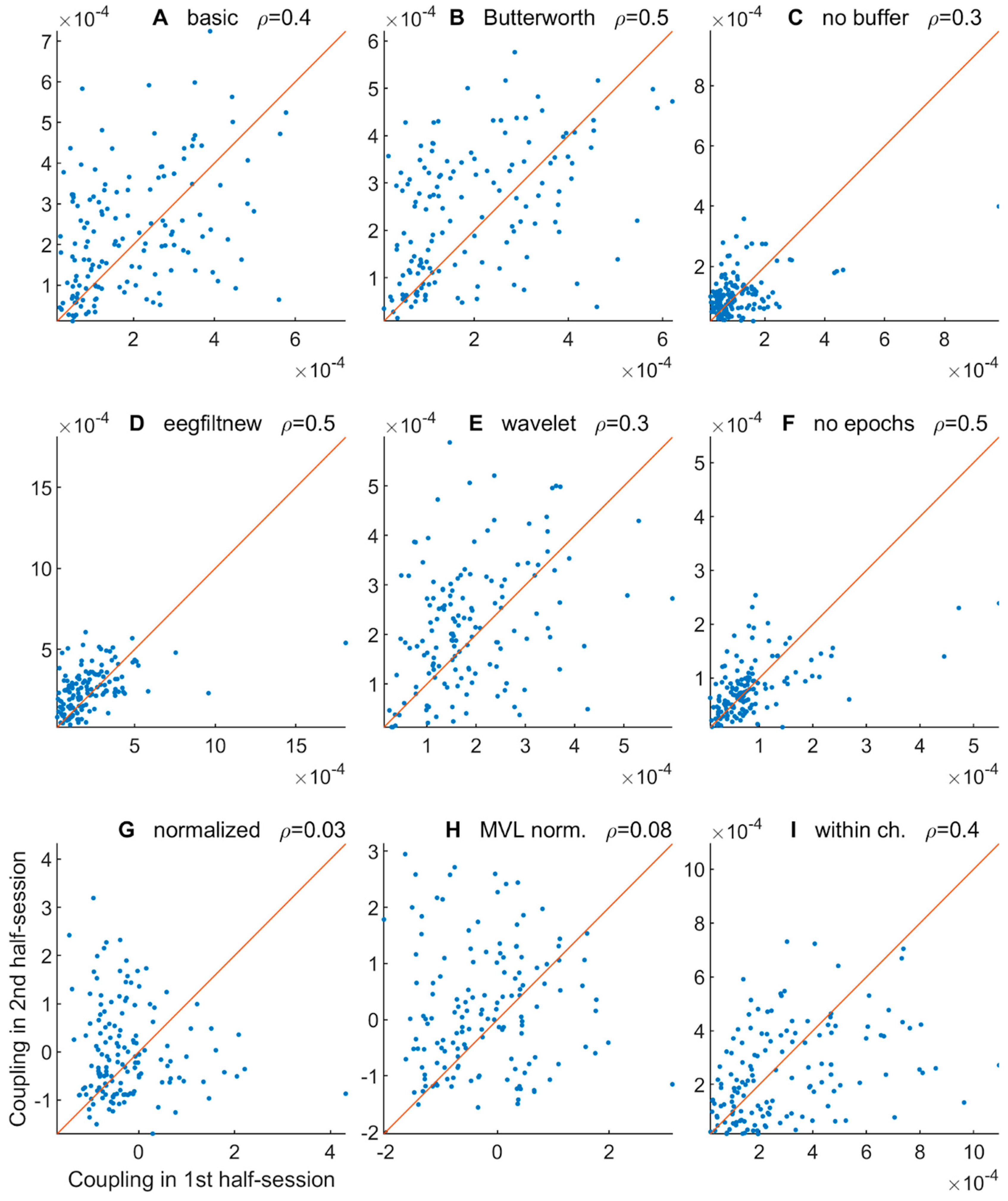
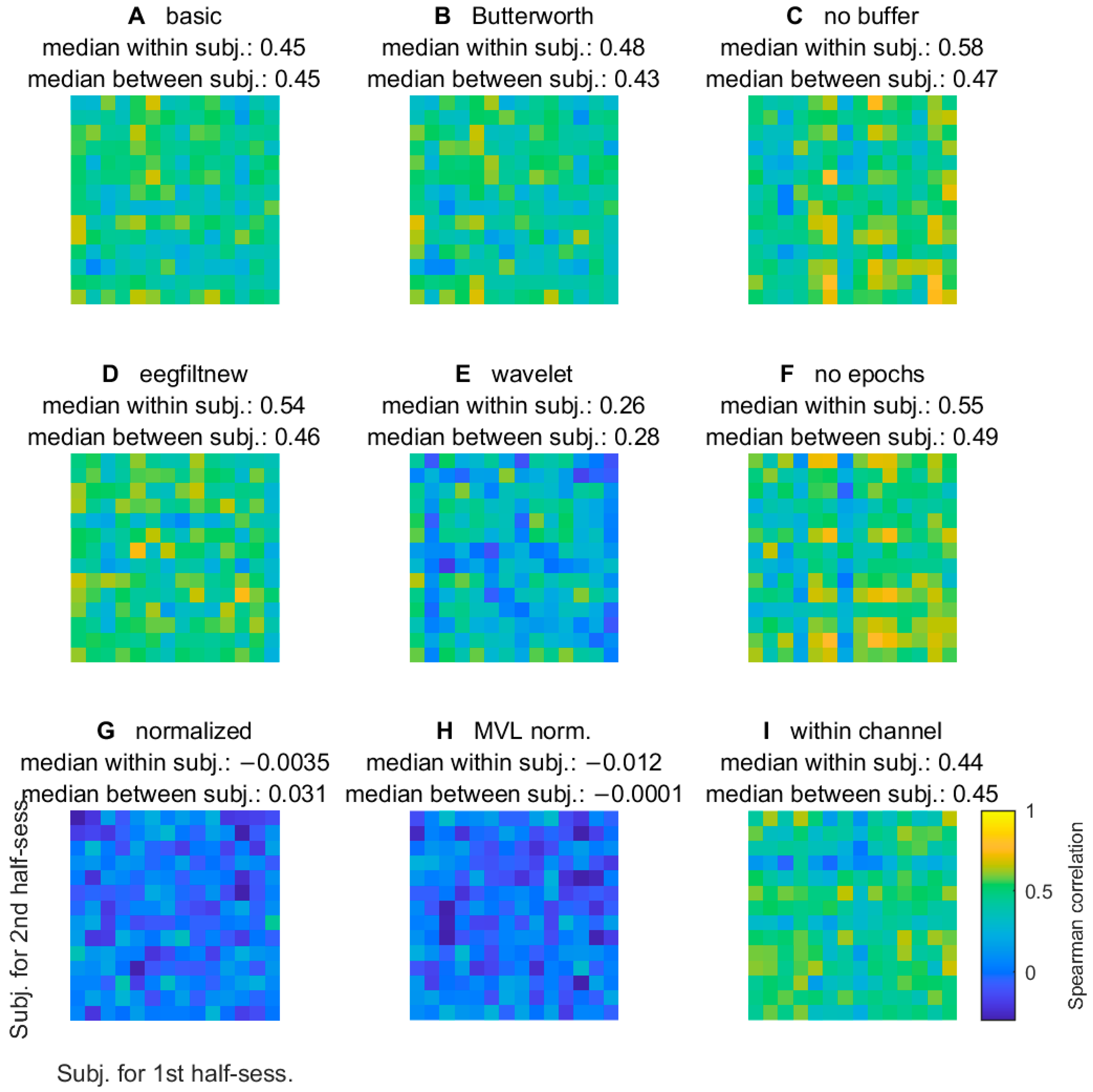
3.2.5. Comodulogram Variability between Half-Sessions

The overall appearance of comodulograms for EEG differed considerably both between the half-sessions and between the PAC calculation algorithms (Figure 7), although some of the peaks appeared to be consistent. In some cases, there was one dominant maximum, and in others, the comodulogram contained several peaks of comparable intensity.

The scatter plots between the comodulograms in the half-sessions showed a degree of reproducibility that ranged from moderate to low in the different methods (Figure 8).

The Spearman correlation coefficients of the comodulograms from the half-sessions were calculated for each subject and method, and their histograms (empirical distributions) are shown in Figure 9. For all methods except the normalized ones, the median correlations were significantly above zero. Thus, for these methods, the comodulograms in the half-sessions on average have some degree of overall similarity.

To check whether only the comodulograms of the same subject were similar rather than all comodulograms from any subject, we compared the within-subject and between-subject correlations of the half-sessions, which are represented by the diagonal and off-diagonal values in the matrices shown in Figure 10. A possible weak tendency towards larger within-subject than between-subject correlations was observed for the methods ‘Butterworth’, ‘no buffer’, ‘eegfitlnew’, and ‘no epochs’ (difference in medians 0.05–0.11). For the other methods, the correlations were close (difference in medians 0–0.02), consistent with the unspecific similarity of all comodulograms.

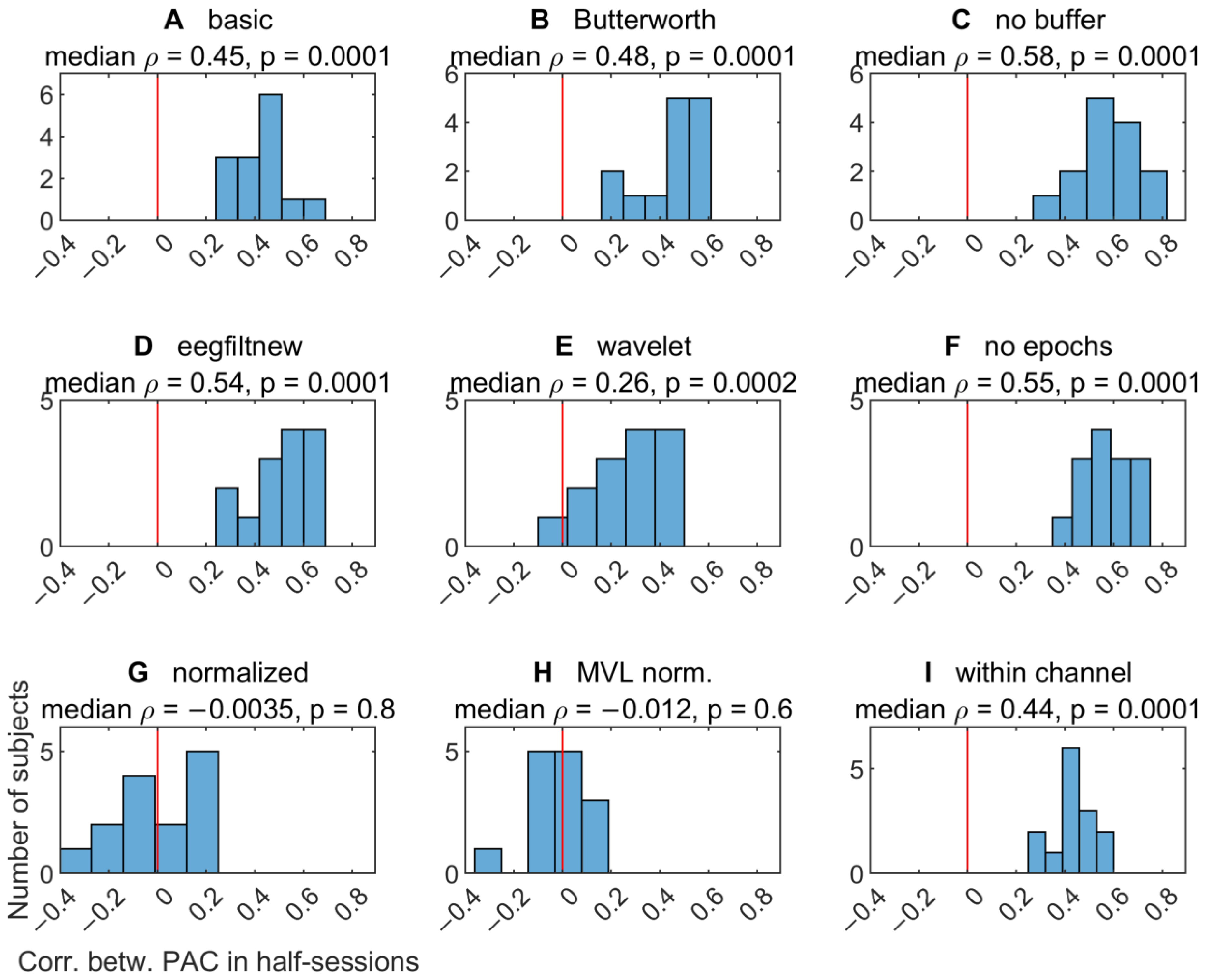
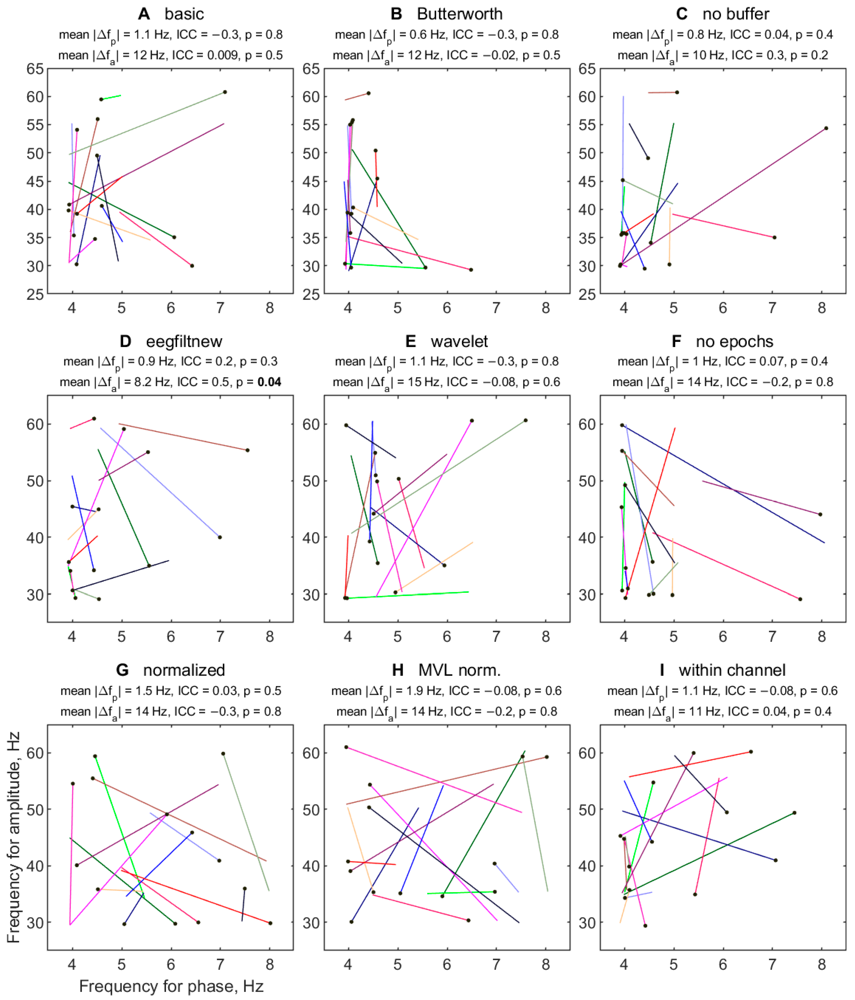
3.2.6. Variability of TGC Peak Frequencies between Half-Sessions

The TGC peaks in the half-sessions showed large variability both between half-sessions and between the algorithms (Figure 11). The mean absolute frequency changes between half-sessions ranged from 0.6 to 1.9 Hz for phase and from 8.2 to 15 Hz for amplitude. These changes differed significantly between the algorithms for the phase frequency (Friedman’s test, p = 0.04), but not the amplitude frequency. The post-hoc tests (Tukey–Kramer) showed that the absolute phase frequency shifts in the ‘Butterworth’ method were smaller than in the ‘MVL normalized’ method (p = 0.049, median of the differences −1 Hz), with no other significant differences.

The ICC values for the peak frequencies ranged from −0.3 to 0.5, and the tests against zero produced p > 0.05 for all of them except for the amplitude frequency in the method ‘eegfiltnew’ (ICC = 0.5, p = 0.04).

3.2.7. Effect of Half-Session on TGC Peak Frequencies

The peak frequencies for both phase and amplitude did not significantly differ on average between the two half-sessions (Wilcoxon’s signed-rank test, p > 0.05 for all the algorithms), suggesting no systematic influence on the frequencies from aspects such as fatigue or learning during the session.

4. Discussion

We examined the reproducibility of theta-gamma coupling between repeated measurements using a set of EEG data for healthy subjects performing the 3-back working memory task as well as a publicly available benchmark LFP recording with previously reported strong PAC. The analysis was concerned with the overall structure of the comodulograms and the frequencies of maximal TGC, in view of the possibility of using these frequencies in customizing noninvasive neuromodulation techniques to optimally impact the neural dynamics of every individual subject. For studying repeatability, the results of processing the two halves of each recording were treated as repeated measurements. Thus, the findings pertain to TGC reproducibility at short time intervals comparable to the session length (a few minutes).

Several PAC calculation pipelines (Table 1 and Table 2) were compared in terms of their influence on the obtained coupling patterns, peak frequencies, and their temporal stability. The algorithms were constructed on the basis of an analysis of the approaches to TGC estimation used in the literature and the available options at each step of the computation. A number of these options have previously been compared on synthetic data, while there is insufficient information about their influence on PAC estimates for actual neural signals.

The benchmark LFP data from the rat hippocampus showed a large theta peak in the power spectrum that was repeatable between the half-sessions (Figure 2). The comodulograms were largely similar between the considered algorithms, although there were noticeable peak differences in certain methods (Figure 3). A considerable degree of reproducibility between the half-sessions was found for both the general shape of the comodulograms (measured by the Spearman correlations) and the positions of PAC maxima in them (quantified by the peak frequency changes, Figure 4 and Figure 5, with absolute values 0–2.5 Hz for phase and 0–5 Hz for amplitude). Each considered algorithm of PAC computation produced one bright peak, all of them having roughly similar locations but varying shapes, with relatively broad and ‘patchy’ peaks for the two methods employing the normalization of the PAC index by surrogate data. It may be possible to smooth these comodulograms using a larger number of surrogates, but, in addition to increased computation time, there is no guarantee that the results will be more repeatable or accurate.

In the EEG data, the presence of theta peaks in electrode Fz was not universal, and many of them were only minimally noticeable against the background (Figure 6). This is largely consistent with previous reports providing variable evidence for theta oscillations during human episodic memory, with some studies reporting memory-related theta increases and others reporting decreases [2]. Thus, a test–retest study [63] of spectra during a modified Sternberg task showed theta peaks in the AFz signal of some but not all subjects. This raises concerns about the range of applicability of TGC analysis because the existence of a clear peak at the frequency for phase is recognized as a prerequisite for a meaningful interpretation of any CFC pattern [25].

The TGC comodulograms generally showed a considerable variation both between the algorithms and between half-sessions (Figure 7 and Figure 8). The Spearman correlations of the comodulograms between half-sessions did not significantly differ on average from zero for the two methods that include normalization, while a significant positive average comodulogram similarity was found for the other methods (Figure 9). However, to a large degree, this was not specific to the particular individual. Indeed, the similarity of comodulograms from different subjects was comparable to that of comodulograms from the same participant (Figure 10).

The fact that the methods using unnormalized KL-MI, unlike the algorithms with normalization, produced comodulograms with significant ‘unspecific’ similarity (both within and between individuals) presents interest for further research. At least a partial explanation of this may be the apparent tendency of the unnormalized KL-MI to find higher PAC values at low phase frequencies, which can be observed from the concentration of the PAC peaks in the left parts of the windows in Figure 11A–F,I (in contrast to Figure 11G,H for the normalized indices). Being apparently unspecific to a particular dataset, this tendency may also be present in the surrogate comodulograms and thus be removed by the normalization. In line with this tendency is the observation of significantly lower average peak phase frequencies for the (unnormalized) ‘basic’ and ‘Butterworth’ methods than for the ‘normalized MVL’ method, although these algorithms differ not only in the normalization but also in the PAC measure (KL-MI in the ‘basic’ and ‘Butterworth’ methods). Overall, the possible systematic biases of PAC calculation methods towards higher or lower PAC for different frequency ranges need further investigation, including theory and simulations, because the identification of a PAC maximum requires an unbiased comparison between PAC values at different frequencies.

The PAC peak frequencies for EEG showed absolute variability that was comparable to that in the benchmark LFP data for the phase frequency (mean change 0.6–1.9 Hz), but larger variability in the amplitude frequency (8.2–15 Hz). Crucially, their relative reliability measured by the ICC was found to be poor, as the ICCs did not differ significantly from zero (the only result with uncorrected p < 0.05 was p = 0.04 for the ICC of the amplitude frequency in the ‘eegfiltnew’ algorithm, which cannot be considered reliable in view of the number of tests performed).

Taken together, these results demonstrate poor reproducibility of the comodulograms and their peaks for all the considered methods applied to EEG during the 3-back task. With all the ICCs being non-significant, the results do not point to any of the algorithms as producing the most reliable results. That said, in the present sample, the highest ICC estimates were obtained for the ‘eegfiltnew’ algorithm (0.2 and 0.5 for phase and amplitude), making it a promising starting point for further methodological exploration on independent datasets.

The unreliability of the TGC peak frequencies presents a substantial challenge to the validity of using them for personalizing neuromodulation protocols in the considered setting. Indeed, this use relies on the TGC measurement procedure for capturing the individual deviations from the population mean that are stable at least during the time period of the study. The statistical insignificance of the ICCs suggests that even if such deviations do exist, their presence cannot be reliably inferred from the data due to the high trial-to-trial variability.

There are several possible directions that one could investigate aimed at improving this situation. First, the range of algorithms for PAC computation can be further expanded. We mainly varied one aspect of the algorithm at a time while keeping the remaining aspects as in the ‘basic’ method (taken from the scripts deposited by A. Tort et al.). However, every option in every step can be combined with any choice in the other steps. This creates a vast space of algorithms, and it is possible that some combinations are better at extracting the stable parts of PAC patterns.

Second, the length of the recording can be increased. The authors of the study [23] suggest that “each laboratory should perform its own control analysis to assess the minimal data length providing a reliable measurement”. However, increasing data length may or may not make the frequencies more stable, because prolonged sessions can induce fatigue effects, while merging data from different occasions may introduce heterogeneities due to temporal effects such as time of day.

Third, one can vary the cognitive task or eliminate it (i.e., investigate the resting state). In the latter case, with eyes closed, the study [18] found between-session reproducibility comparable to our results for the n-back task. The Spearman correlation between gamma frequencies in two sessions was reported to be 0.32, while the value of the insignificant correlation between theta frequencies was not reported, but we calculated it from supplementary data as 0.01. The authors concluded that “inconsistent results within subjects suggest that theta and gamma cycle lengths and their ratio may be a state marker rather than a stable trait marker”, which is a possible explanation of our results as well. However, there is still a possibility that some other tasks will induce more stable neural dynamics.

Finally, perhaps the most promising way forward is to explore the possibility that TGC may be unstable but still important, and target it using the closed-loop approach, where the stimulation is continuously adjusted on the basis of the simultaneously measured neural activity [64,65]. To this end, it is important to investigate algorithms for online estimation of the currently dominant PAC frequencies. One of the tools that may help in this regard is deep learning, due to its ability to adaptively extract information from EEG signals [66,67,68], which may aid in dealing with short data segments.

A limitation of this study is the moderate sample size. However, it is sufficient to detect strong correlations between measurements, which are likely to be required for the individualization of noninvasive stimulation to have considerable advantages. In other words, a larger sample could enable us to estimate the correlations more accurately, and possibly even obtain statistically significant ICCs; however, given the present results, the values of these ICCs are unlikely to be high, and this is what is important in the context of the personalization of brain stimulation.

5. Conclusions

The set of algorithms for PAC calculation explored in this study yielded largely reproducible comodulograms and frequencies of maximal coupling for the benchmark rat LFP data but not for human scalp EEG during the n-back working memory task. More research is needed on the algorithms, cognitive tasks, minimal data length, and alternative conceptual approaches to determine and effectively use theta-gamma coupling parameters in adapting neuromodulation to the internal dynamics of brain signals.

References

1. Buzsáki, G.; Watson, B.O. Brain Rhythms and Neural Syntax: Implications for Efficient Coding of Cognitive Content and Neuropsychiatric Disease. Dialogues Clin. Neurosci. 2012, 14, 345–367. [Google Scholar] [CrossRef] [PubMed]
2. Herweg, N.A.; Solomon, E.A.; Kahana, M.J. Theta Oscillations in Human Memory. Trends Cogn. Sci. 2020, 24, 208–227. [Google Scholar] [CrossRef] [PubMed]
3. Sato, Y.; Schmitt, O.; Ip, Z.; Rabiller, G.; Omodaka, S.; Tominaga, T.; Yazdan-Shahmorad, A.; Liu, J. Pathological Changes of Brain Oscillations Following Ischemic Stroke. J. Cereb. Blood Flow Metab. 2022, 42, 1753–1776. [Google Scholar] [CrossRef] [PubMed]
4. Giustiniani, A.; Danesin, L.; Bozzetto, B.; Macina, A.; Benavides-Varela, S.; Burgio, F. Functional Changes in Brain Oscillations in Dementia: A Review. Rev. Neurosci. 2023, 34, 25–47. [Google Scholar] [CrossRef] [PubMed]
5. Bragin, A.; Jandó, G.; Nádasdy, Z.; Hetke, J.; Wise, K.; Buzsáki, G. Gamma (40–100 Hz) Oscillation in the Hippocampus of the Behaving Rat. J. Neurosci. 1995, 15, 47–60. [Google Scholar] [CrossRef]
6. Lakatos, P.; Shah, A.S.; Knuth, K.H.; Ulbert, I.; Karmos, G.; Schroeder, C.E. An Oscillatory Hierarchy Controlling Neuronal Excitability and Stimulus Processing in the Auditory Cortex. J. Neurophysiol. 2005, 94, 1904–1911. [Google Scholar] [CrossRef]
7. Canolty, R.T.; Edwards, E.; Dalal, S.S.; Soltani, M.; Nagarajan, S.S.; Kirsch, H.E.; Berger, M.S.; Barbaro, N.M.; Knight, R.T. High Gamma Power Is Phase-Locked to Theta Oscillations in Human Neocortex. Science (1979) 2006, 313, 1626–1628. [Google Scholar] [CrossRef]
8. Park, J.Y.; Lee, Y.-R.; Lee, J. The Relationship between Theta-Gamma Coupling and Spatial Memory Ability in Older Adults. Neurosci. Lett. 2011, 498, 37–41. [Google Scholar] [CrossRef]
9. Abubaker, M.; Al Qasem, W.; Kvašňák, E. Working Memory and Cross-Frequency Coupling of Neuronal Oscillations. Front. Psychol. 2021, 12, 756661. [Google Scholar] [CrossRef]
10. Fell, J.; Axmacher, N. The Role of Phase Synchronization in Memory Processes. Nat. Rev. Neurosci. 2011, 12, 105–118. [Google Scholar] [CrossRef]
11. Hirano, S.; Nakhnikian, A.; Hirano, Y.; Oribe, N.; Kanba, S.; Onitsuka, T.; Levin, M.; Spencer, K.M. Phase-Amplitude Coupling of the Electroencephalogram in the Auditory Cortex in Schizophrenia. Biol. Psychiatry Cogn. Neurosci. Neuroimaging 2018, 3, 69–76. [Google Scholar] [CrossRef] [PubMed]
12. Brooks, H.; Goodman, M.S.; Bowie, C.R.; Zomorrodi, R.; Blumberger, D.M.; Butters, M.A.; Daskalakis, Z.J.; Fischer, C.E.; Flint, A.; Herrmann, N.; et al. Theta–Gamma Coupling and Ordering Information: A Stable Brain–Behavior Relationship across Cognitive Tasks and Clinical Conditions. Neuropsychopharmacology 2020, 45, 2038–2047. [Google Scholar] [CrossRef] [PubMed]
13. Lisman, J.E.; Idiart, M.A.P. Storage of 7 ± 2 Short-Term Memories in Oscillatory Subcycles. Science (1979) 1995, 267, 1512–1515. [Google Scholar] [CrossRef] [PubMed]
14. De Almeida, L.; Idiart, M.; Villavicencio, A.; Lisman, J. Alternating Predictive and Short-Term Memory Modes of Entorhinal Grid Cells. Hippocampus 2012, 22, 1647–1651. [Google Scholar] [CrossRef] [PubMed]
15. Lisman, J.E.; Jensen, O. The Theta-Gamma Neural Code. Neuron 2013, 77, 1002–1016. [Google Scholar] [CrossRef] [PubMed]
16. Miller, G.A. The Magical Number Seven, plus or Minus Two: Some Limits on Our Capacity for Processing Information. Psychol. Rev. 1956, 63, 81–97. [Google Scholar] [CrossRef] [PubMed]
17. Kamiński, J.; Brzezicka, A.; Wróbel, A. Short-Term Memory Capacity (7±2) Predicted by Theta to Gamma Cycle Length Ratio. Neurobiol. Learn. Mem. 2011, 95, 19–23. [Google Scholar] [CrossRef] [PubMed]
18. Malenínská, K.; Rudolfová, V.; Šulcová, K.; Koudelka, V.; Brunovský, M.; Horáček, J.; Nekovářová, T. Is Short-Term Memory Capacity (7 ± 2) Really Predicted by Theta to Gamma Cycle Length Ratio? Behav. Brain Res. 2021, 414, 113465. [Google Scholar] [CrossRef]
19. Poydasheva, A.G.; Bakulin, I.S.; Sinitsyn, D.O.; Zabirova, A.H.; Lagoda, D.Y.; Suponeva, N.A.; Piradov, M.A. Theta-Gamma Phase-Amplitude Coupling: Physiological Basics, Analysis Methods, and Perspectives of Translation into Clinical Practice. Ann. Clin. Exp. Neurol. 2022, 16, 71–79. [Google Scholar] [CrossRef]
20. Vosskuhl, J.; Huster, R.J.; Herrmann, C.S. Increase in Short-Term Memory Capacity Induced by down-Regulating Individual Theta Frequency via Transcranial Alternating Current Stimulation. Front. Hum. Neurosci. 2015, 9, 257. [Google Scholar] [CrossRef]
21. Chung, S.W.; Sullivan, C.M.; Rogasch, N.C.; Hoy, K.E.; Bailey, N.W.; Cash, R.F.H.; Fitzgerald, P.B. The Effects of Individualised Intermittent Theta Burst Stimulation in the Prefrontal Cortex: A TMS-EEG Study. Hum. Brain Mapp. 2019, 40, 608–627. [Google Scholar] [CrossRef] [PubMed]
22. Penny, W.D.; Duzel, E.; Miller, K.J.; Ojemann, J.G. Testing for Nested Oscillation. J. Neurosci. Methods 2008, 174, 50–61. [Google Scholar] [CrossRef] [PubMed]
23. Tort, A.B.L.; Komorowski, R.; Eichenbaum, H.; Kopell, N. Measuring Phase-Amplitude Coupling Between Neuronal Oscillations of Different Frequencies. J. Neurophysiol. 2010, 104, 1195–1210. [Google Scholar] [CrossRef]
24. Dvorak, D.; Fenton, A.A. Toward a Proper Estimation of Phase–Amplitude Coupling in Neural Oscillations. J. Neurosci. Methods 2014, 225, 42–56. [Google Scholar] [CrossRef] [PubMed]
25. Aru, J.; Aru, J.; Priesemann, V.; Wibral, M.; Lana, L.; Pipa, G.; Singer, W.; Vicente, R. Untangling Cross-Frequency Coupling in Neuroscience. Curr. Opin. Neurobiol. 2015, 31, 51–61. [Google Scholar] [CrossRef] [PubMed]
26. Seymour, R.A.; Rippon, G.; Kessler, K. The Detection of Phase Amplitude Coupling during Sensory Processing. Front. Neurosci. 2017, 11, 487. [Google Scholar] [CrossRef] [PubMed]
27. Hülsemann, M.J.; Naumann, E.; Rasch, B. Quantification of Phase-Amplitude Coupling in Neuronal Oscillations: Comparison of Phase-Locking Value, Mean Vector Length, Modulation Index, and Generalized-Linear-Modeling-Cross-Frequency-Coupling. Front. Neurosci. 2019, 13, 573. [Google Scholar] [CrossRef]
28. Caiola, M.; Devergnas, A.; Holmes, M.H.; Wichmann, T. Empirical Analysis of Phase-Amplitude Coupling Approaches. PLoS ONE 2019, 14, e0219264. [Google Scholar] [CrossRef]
29. Combrisson, E.; Nest, T.; Brovelli, A.; Ince, R.A.A.; Soto, J.L.P.; Guillot, A.; Jerbi, K. Tensorpac: An Open-Source Python Toolbox for Tensor-Based Phase-Amplitude Coupling Measurement in Electrophysiological Brain Signals. PLoS Comput. Biol. 2020, 16, e1008302. [Google Scholar] [CrossRef]
30. Matlab Routines for Computing the Modulation Index and Comodulogram, as Described in Tort et al., J Neurophysiol 2010. Available online: https://github.com/tortlab/phase-amplitude-coupling (accessed on 2 October 2023).
31. Scheffer-Teixeira, R.; Belchior, H.; Caixeta, F.V.; Souza, B.C.; Ribeiro, S.; Tort, A.B.L. Theta Phase Modulates Multiple Layer-Specific Oscillations in the CA1 Region. Cerebral Cortex 2012, 22, 2404–2414. [Google Scholar] [CrossRef]
32. Delorme, A.; Makeig, S. EEGLAB: An Open Source Toolbox for Analysis of Single-Trial EEG Dynamics Including Independent Component Analysis. J. Neurosci. Methods 2004, 134, 9–21. [Google Scholar] [CrossRef] [PubMed]
33. Friese, U.; Köster, M.; Hassler, U.; Martens, U.; Trujillo-Barreto, N.; Gruber, T. Successful Memory Encoding Is Associated with Increased Cross-Frequency Coupling between Frontal Theta and Posterior Gamma Oscillations in Human Scalp-Recorded EEG. Neuroimage 2013, 66, 642–647. [Google Scholar] [CrossRef] [PubMed]
34. Köster, M.; Friese, U.; Schöne, B.; Trujillo-Barreto, N.; Gruber, T. Theta-Gamma Coupling during Episodic Retrieval in the Human EEG. Brain Res. 2014, 1577, 57–68. [Google Scholar] [CrossRef] [PubMed]
35. Musaeus, C.S.; Nielsen, M.S.; Musaeus, J.S.; Høgh, P. Electroencephalographic Cross-Frequency Coupling as a Sign of Disease Progression in Patients With Mild Cognitive Impairment: A Pilot Study. Front. Neurosci. 2020, 14, 790. [Google Scholar] [CrossRef] [PubMed]
36. Gong, R.; Wegscheider, M.; Mühlberg, C.; Gast, R.; Fricke, C.; Rumpf, J.-J.; Nikulin, V.V.; Knösche, T.R.; Classen, J. Spatiotemporal Features of β-γ Phase-Amplitude Coupling in Parkinson’s Disease Derived from Scalp EEG. Brain 2021, 144, 487–503. [Google Scholar] [CrossRef] [PubMed]
37. Rajji, T.K.; Zomorrodi, R.; Barr, M.S.; Blumberger, D.M.; Mulsant, B.H.; Daskalakis, Z.J. Ordering Information in Working Memory and Modulation of Gamma by Theta Oscillations in Humans. Cereb. Cortex 2017, 27, 1482–1490. [Google Scholar] [CrossRef]
38. Goodman, M.S.; Kumar, S.; Zomorrodi, R.; Ghazala, Z.; Cheam, A.S.M.; Barr, M.S.; Daskalakis, Z.J.; Blumberger, D.M.; Fischer, C.; Flint, A.; et al. Theta-Gamma Coupling and Working Memory in Alzheimer’s Dementia and Mild Cognitive Impairment. Front. Aging Neurosci. 2018, 10, 101. [Google Scholar] [CrossRef]
39. Rustamov, N.; Humphries, J.; Carter, A.; Leuthardt, E.C. Theta-Gamma Coupling as a Cortical Biomarker of Brain-Computer Interface-Mediated Motor Recovery in Chronic Stroke. Brain Commun. 2022, 4, fcac136. [Google Scholar] [CrossRef]
40. Park, J.Y.; Jhung, K.; Lee, J.; An, S.K. Theta-Gamma Coupling during a Working Memory Task as Compared to a Simple Vigilance Task. Neurosci. Lett. 2013, 532, 39–43. [Google Scholar] [CrossRef]
41. Sun, Y.; Giacobbe, P.; Tang, C.W.; Barr, M.S.; Rajji, T.; Kennedy, S.H.; Fitzgerald, P.B.; Lozano, A.M.; Wong, W.; Daskalakis, Z.J. Deep Brain Stimulation Modulates Gamma Oscillations and Theta-Gamma Coupling in Treatment Resistant Depression. Brain Stimul. 2015, 8, 1033–1042. [Google Scholar] [CrossRef]
42. Köster, M.; Finger, H.; Graetz, S.; Kater, M.; Gruber, T. Theta-Gamma Coupling Binds Visual Perceptual Features in an Associative Memory Task. Sci. Rep. 2018, 8, 17688. [Google Scholar] [CrossRef] [PubMed]
43. Jones, K.T.; Johnson, E.L.; Berryhill, M.E. Frontoparietal Theta-Gamma Interactions Track Working Memory Enhancement with Training and TDCS. Neuroimage 2020, 211, 116615. [Google Scholar] [CrossRef] [PubMed]
44. Swann, N.C.; De Hemptinne, C.; Aron, A.R.; Ostrem, J.L.; Knight, R.T.; Starr, P.A. Elevated Synchrony in Parkinson Disease Detected with Electroencephalography. Ann. Neurol. 2015, 78, 742–750. [Google Scholar] [CrossRef] [PubMed]
45. Hammer, M.; Schwale, C.; Brankačk, J.; Draguhn, A.; Tort, A.B.L. Theta-Gamma Coupling during REM Sleep Depends on Breathing Rate. Sleep 2021, 44, zsab189. [Google Scholar] [CrossRef] [PubMed]
46. Miyakoshi, M.; Delorme, A.; Mullen, T.; Kojima, K.; Makeig, S.; Asano, E. Automated Detection of Cross-Frequency Coupling in the Electrocorticogram for Clinical Inspection. In Proceedings of the 2013 35th Annual International Conference of the IEEE Engineering in Medicine and Biology Society (EMBC), Osaka, Japan, 3–7 July 2013; pp. 3282–3285. [Google Scholar]
47. Attaheri, A.; Choisdealbha, N.; Di Liberto, G.M.; Rocha, S.; Brusini, P.; Mead, N.; Olawole-Scott, H.; Boutris, P.; Gibbon, S.; Williams, I.; et al. Delta- and Theta-Band Cortical Tracking and Phase-Amplitude Coupling to Sung Speech by Infants. Neuroimage 2022, 247, 118698. [Google Scholar] [CrossRef] [PubMed]
48. Widmann, A.; Schröger, E.; Maess, B. Digital Filter Design for Electrophysiological Data-a Practical Approach. J. Neurosci. Methods 2015, 250, 34–46. [Google Scholar] [CrossRef] [PubMed]
49. Dupré la Tour, T.; Tallot, L.; Grabot, L.; Doyère, V.; van Wassenhove, V.; Grenier, Y.; Gramfort, A. Non-Linear Auto-Regressive Models for Cross-Frequency Coupling in Neural Time Series. PLoS Comput. Biol. 2017, 13, e1005893. [Google Scholar] [CrossRef] [PubMed]
50. Cohen, M.X. Analyzing Neural Time Series Data: Theory and Practice; MIT Press: Cambridge, MA, USA, 2014. [Google Scholar]
51. Axmacher, N.; Henseler, M.M.; Jensen, O.; Weinreich, I.; Elger, C.E.; Fell, J. Cross-Frequency Coupling Supports Multi-Item Working Memory in the Human Hippocampus. Proc. Natl. Acad. Sci. USA 2010, 107, 3228–3233. [Google Scholar] [CrossRef]
52. Papaioannou, O.; Crespo, L.P.; Clark, K.; Ogbuagu, N.N.; Alliende, L.M.; Silverstein, S.M.; Erickson, M.A. Is Cortical Theta-Gamma Phase-Amplitude Coupling Memory-Specific? Brain Sci. 2022, 12, 1131. [Google Scholar] [CrossRef]
53. Tallon-Baudry, C.; Bertrand, O.; Delpuech, C.; Pernier, J. Oscillatory γ-Band (30–70 Hz) Activity Induced by a Visual Search Task in Humans. J. Neurosci. 1997, 17, 722–734. [Google Scholar] [CrossRef]
54. Martinez-Cancino, R.; Delorme, A.; Kreutz-Delgado, K.; Makeig, S. Computing Phase Amplitude Coupling in EEGLAB: PACTools. In Proceedings of the IEEE 20th International Conference on Bioinformatics and Bioengineering, BIBE 2020, Cincinnati, OH, USA, 26–28 October 2020. [Google Scholar]
55. Özkurt, T.E.; Schnitzler, A. A Critical Note on the Definition of Phase-Amplitude Cross-Frequency Coupling. J. Neurosci. Methods 2011, 201, 438–443. [Google Scholar] [CrossRef] [PubMed]
56. Heninger, G.R.; Mcdonald, R.K.; Goff, W.R.; Sollberger, A. Diurnal Variations in the Cerebral Evoked Response and EEG: Relations to 17-Hydroxycorticosteroid Levels. Arch. Neurol. 1969, 21, 330–337. [Google Scholar] [CrossRef] [PubMed]
57. Sheehan, K.A.; McArthur, G.M.; Bishop, D.V.M. Is Discrimination Training Necessary to Cause Changes in the P2 Auditory Event-Related Brain Potential to Speech Sounds? Cogn. Brain Res. 2005, 25, 547–553. [Google Scholar] [CrossRef] [PubMed]
58. Bhangal, S.; Sharma, S.; Valle-Inclán, F.; Ren, X.; Hackley, S.A. Learning to Deal with Delayed Outcomes: EEG Oscillatory and Slow Potentials during the Prefeedback Interval. Psychophysiology 2021, 58, e13853. [Google Scholar] [CrossRef] [PubMed]
59. Nawaz, R.; Wood, G.; Nisar, H.; Yap, V.V. Exploring the Effects of EEG-Based Alpha Neurofeedback on Working Memory Capacity in Healthy Participants. Bioengineering 2023, 10, 200. [Google Scholar] [CrossRef] [PubMed]
60. Maheshwari, A.; Akbar, A.; Wang, M.; Marks, R.L.; Yu, K.; Park, S.; Foster, B.L.; Noebels, J.L. Persistent Aberrant Cortical Phase–Amplitude Coupling Following Seizure Treatment in Absence Epilepsy Models. J. Physiol. 2017, 595, 7249–7260. [Google Scholar] [CrossRef]
61. McGraw, K.O.; Wong, S.P. Forming Inferences about Some Intraclass Correlation Coefficients. Psychol. Methods 1996, 1, 30–46. [Google Scholar] [CrossRef]
62. Salarian, A. Intraclass Correlation Coefficient (ICC), MATLAB Central File Exchange. 2023. Available online: https://www.mathworks.com/matlabcentral/fileexchange/22099-intraclass-correlation-coefficient-icc (accessed on 3 October 2023).
63. Näpflin, M.; Wildi, M.; Sarnthein, J. Test-Retest Reliability of EEG Spectra during a Working Memory Task. Neuroimage 2008, 43, 687–693. [Google Scholar] [CrossRef]
64. Gordon, P.C.; Belardinelli, P.; Stenroos, M.; Ziemann, U.; Zrenner, C. Prefrontal Theta Phase-Dependent RTMS-Induced Plasticity of Cortical and Behavioral Responses in Human Cortex. Brain Stimul. 2022, 15, 391–402. [Google Scholar] [CrossRef]
65. Zrenner, C.; Ziemann, U. Closed-Loop Stimulation. Biol. Psychiatry 2023, in press. [Google Scholar] [CrossRef]
66. Jia, Z.; Lin, Y.; Wang, J.; Ning, X.; He, Y.; Zhou, R.; Zhou, Y.; Lehman, L.H. Multi-View Spatial-Temporal Graph Convolutional Networks With Domain Generalization for Sleep Stage Classification. IEEE Trans. Neural Syst. Rehabil. Eng. 2021, 29, 1977–1986. [Google Scholar] [CrossRef] [PubMed]
67. Jia, Z.; Cai, X.; Jiao, Z. Multi-Modal Physiological Signals Based Squeeze-and-Excitation Network With Domain Adversarial Learning for Sleep Staging. IEEE Sens. J. 2022, 22, 3464–3471. [Google Scholar] [CrossRef]
68. Jia, Z.; Ji, J.; Zhou, X.; Zhou, Y. Hybrid Spiking Neural Network for Sleep Electroencephalogram Signals. Sci. China Inf. Sci. 2022, 65, 140403. [Google Scholar] [CrossRef]
Figure 1. Structure of the 3-back task.
Algorithms 16 00540 g001
Figure 2. Power spectral density for the benchmark LFP data, computed from half-sessions. The dots denote the peaks at 8 and 8.5 Hz in the first and second half-sessions, respectively.
Algorithms 16 00540 g002
Figure 3. Comodulograms for the benchmark LFP data from the whole session calculated using different algorithms (AI) described in Table 1. The red circle in each plot shows the point of maximal PAC in the current algorithm, and the black circle shows the peak from the ‘basic’ method (A) for comparison (invisible in B due to both peaks coinciding). The differences of the peak frequencies from the ones in the ‘basic’ method (7.5 and 80 Hz) are indicated (subscripts ‘p’ and ‘a’ correspond to phase and amplitude, here and below).
Algorithms 16 00540 g003
Figure 4. Comodulograms computed from half-sessions of the benchmark LFP data by the ‘basic’ algorithm (A) and the ‘simulated epochs’ algorithm (B) described in Table 1 (note that the plot letter B here differs from this method’s letter I in the table). The red circle in each plot shows the point of maximal PAC. The black circle in each comodulogram for the 2nd half-session shows the peak from the 1st half-session for comparison (invisible in A due to both peaks coinciding). The differences between the peak frequencies in the half-sessions are indicated.
Algorithms 16 00540 g004
Figure 5. Comparison of PAC measures between the half-sessions of the benchmark LFP data, with PAC calculated by the methods from Table 1 (AI). Each circle corresponds to one point in a comodulogram, i.e., to a pair of frequency bands for phase and amplitude. The orange line “y = x” corresponds to equal coupling in the two half-sessions (exact reproducibility). The Spearman correlation coefficients of PAC values (ρ) and peak frequency changes between the half-sessions are indicated.
Algorithms 16 00540 g005
Figure 6. Power spectral density for the EEG signals in electrode Fz for each of the subjects performing the 3-back task. The spectra were calculated from the ‘VEP-free’ epochs (500–3000 ms from stimulus onset) within the first half-session (blue lines) and the second one (orange lines). The gray vertical lines define the 4–8 Hz theta range, and the circles denote the highest local maxima in this range (where such maxima exist).
Algorithms 16 00540 g006
Figure 7. Comodulograms for half-sessions of one subject (selected to have average TGC peak variability as described in the Methods section). The results in figures (AI) were obtained from the same data by the different PAC calculation methods described in Table 2. The red dot in each plot shows the point of maximal PAC. The black dot in each comodulogram for the 2nd half-session shows the peak from the 1st half-session for comparison. Note: to provide more detail for coupling in the considered theta-gamma frequency window (shown by the white dashed rectangle), the color scale in each plot was chosen to cover the range of PAC values within this window. Values outside this range are shown by a uniform color (yellow or dark blue).
Algorithms 16 00540 g007
Figure 8. Comparison of PAC measures between the half-sessions for the same subject as in Figure 7. The results in figures (AI) were obtained from the same data by the different PAC calculation methods described in Table 2. Each circle corresponds to one point in a comodulogram, i.e., to a pair of frequency bands for phase and amplitude. The orange line “y = x” corresponds to equal coupling in the two half-sessions (exact reproducibility). The Spearman correlation coefficients (ρ) of PAC values between the half-sessions are indicated.
Algorithms 16 00540 g008
Figure 9. Distributions of Spearman correlation coefficients between the comodulograms from half-sessions for each PAC calculation method from Table 2 (AI). Medians are indicated, as are the p-values from Wilcoxon’s signed-rank tests. The red lines correspond to no similarity (ρ = 0).
Algorithms 16 00540 g009
Figure 10. Spearman correlations between comodulograms from the first half-sessions of every subject with the second half-sessions of every other subject, with PAC calculation by the methods from Table 2 (AI). In the case of reproducible and unique patterns in the comodulograms of every subject, the matrices should have large diagonal values (within-subject correlations) and smaller off-diagonal values (between-subject correlations). The corresponding median values are indicated.
Algorithms 16 00540 g010
Figure 11. Positions of TGC peaks in the comodulograms from half-sessions obtained by the different PAC calculation methods from Table 2 (AI) for all subjects. The two peaks for each subject are connected by a line of a unique color, which is consistent between figures (AI). The peak in the first half-session is shown by a black dot. Small jitter was added to the peak coordinates to make most of them distinct. Measures of reproducibility are indicated for the phase and amplitude frequency of the peak: the mean absolute frequency change between the half-sessions and the intraclass correlation coefficient (ICC) of the frequency, along with the p-value for the test of the ICC against zero. The values p < 0.05 are shown in bold.
Algorithms 16 00540 g011