

The Use of Correlation Features in the Problem of Speech Recognition


Data Analysis and Machine Learning Department, Financial University under the Government of the Russian Federation, pr-kt Leningradsky, 49/2, 125167 Moscow, Russia
Algorithms 2023, 16(2), 90; https://doi.org/10.3390/a16020090
Submission received: 30 November 2022
/
Revised: 11 January 2023
/
Accepted: 6 February 2023
/
Published: 7 February 2023
(This article belongs to the Special Issue Algorithms for Feature Selection)
Abstract
:The problem solved in the article is connected with the increase in the efficiency of phraseological radio exchange message recognition, which sometimes takes place in conditions of increased tension for the pilot. For high-quality recognition, signal preprocessing methods are needed. The article considers new data preprocessing algorithms used to extract features from a speech message. In this case, two approaches were proposed. The first approach is building autocorrelation functions of messages based on the Fourier transform, the second one uses the idea of building autocorrelation portraits of speech signals. The proposed approaches are quite simple to implement, although they require cyclic operators, since they work with pairs of samples from the original signal. Approbation of the developed method was carried out with the problem of recognizing phraseological radio exchange messages in Russian. The algorithm with preliminary feature extraction provides a gain of 1.7% in recognition accuracy. The use of convolutional neural networks also provides an increase in recognition efficiency. The gain for autocorrelation portraits processing is about 3–4%. Quantization is used to optimize the proposed models. The algorithm’s performance increased by 2.8 times after the quantization. It was also possible to increase accuracy of recognition by 1–2% using digital signal processing algorithms. An important feature of the proposed algorithms is the possibility of generalizing them to arbitrary data with time correlation. The speech message preprocessing algorithms discussed in this article are based on classical digital signal processing algorithms. The idea of constructing autocorrelation portraits based on the time series of a signal has a novelty. At the same time, this approach ensures high recognition accuracy. However, the study also showed that all the algorithms under consideration perform quite poorly under the influence of strong noise.
1. Introduction
Currently, automatic and automated systems in transport are of particular relevance. On the one hand, today there are already many algorithms for unmanned vehicles [1,2] and unmanned aerial vehicles [3,4,5]. On the other hand, modern deep learning natural language and multimodal models [6,7,8] make it possible to perform intelligent processing of audio data with a sufficiently high accuracy. Many modern smartphones are equipped with voice assistants, but the devices only solve tasks which are not so sensitive to recognition errors. Furthermore, among other things, errors in such compact devices arise due to distillation and simplification of machine learning models [9,10]. Another problem with the use of the considered recognizers is that such gadgets work badly under noise conditions. At the same time, transport security responsibilities include not only the identification of dangerous items of baggage [11,12], but also the tasks of correct and timely air traffic control.
For high-quality and fast organization of air traffic, a specialized language of phraseological radio exchange is used. This, on the one hand, simplifies the task of recognizing a limited number of phrase patterns, but, on the other hand, requires very high accuracy values for automatic implementation. However, the reception and transmission of the speech messages may adversely affect the aircraft pilot. It is clear that the reception is carried out with aircraft and other noises. Therefore, it is necessary to develop high-quality speech message preprocessing algorithms for feature extraction in order to build automated systems for the phraseological messages recognition. Moreover, such a system should be invariant to the gender and personal characteristics of the voice. Finally, efficient preprocessing and processing in real-time is required.
Obviously, the use of passenger transport carries certain risks. This also applies to aviation security. One of the factors that can be distinguished from human factors is pilot fatigue and workload. Thus, the article considers the applied task of reducing the aircraft pilot workload based on automated speech messages recognition. At the same time, radio exchange is the necessary for transmitting and receiving messages from air traffic control to ensure flight safety. Phraseological radio exchange allows dispatchers and pilots to control the situation on the ground and in the air. However, today radio traffic is not absolutely stable. It is often subject to various kinds of interference, which can greatly distort messages. Sometimes this problem deals with duplicating information, but the time spent can affect the level of flight safety. For example, in different conditions information about a flight height level change or an alternate landing airport will be extremely important.
As for the noise-resistant transmission problem, it is possible to use adaptive filtering methods [13,14,15]. Application of simulation algorithms is necessary to analyze the quality of digital signal processing. This will make it possible to impose noise on speech messages, as well as to evaluate the recognition efficiency for various noise and filtration parameters. Finally, both approaches based on mathematical models [16] and deep learning methods [17] can be used for analysis. The next section is devoted to a brief related works review, which concludes with the use of digital signal preprocessing.
2. Related Works and Presentation and Processing of Speech Messages
Speech recognition is a traditional classification task, where there is a limited set of sounds or phonemes. From this point of view, its solution is possible using classification models, as, for example, deep learning, machine learning or rule-based methods. Articles for processing Arabic messages [18,19,20] provide the main ideas for speech signal classification. The task is greatly simplified by reducing the number of classes. This can happen when it is only necessary to determine an emotion [21] or a spectrum of emotions [22] from a voice message.
Recognition of speech messages in Russian is considered in [23,24,25]. However, sound signal processing approaches also consist in the selection of phonemes in a temporal signal [26]. The rule-based phoneme detection approach developed by the authors of [26] allowed them to obtain recognition accuracy above 99%. In [27], methods of working with hierarchical phonemes are already used. This allows authors to filter out non-existent or unlikely combinations of sounds and generally improves the quality of recognition. Methods based on attention are considered in work [28]. At the same time, it was possible to improve the quality of recognition by 5–6%, focusing on vowels.
However, it should be noted that all the presented algorithms operate with pure signals. When it comes to noisy expressions, recognition becomes much more difficult [29,30,31]. In particular, in [29], the recognition accuracy is already only 91%. Work [30] shows that it is important to apply frequency area processing methods to work with noisy messages. In particular, the authors of [29] use the Fourier transform and also use the Gilbert transform for analysis. The training set augmentation approach [31,32] also proves to be effective in the absence of noisy data in the training set. The work [32] is devoted to the augmentation of noisy images, and the approaches considered in [32] can be applied to autocorrelation portraits of voice messages.
Since the recording of a voice message is signal amplitude changing in dependence on time, then time series models are adequate tools for representing voice messages. Traditional methods for time series modeling and processing are covered by the work [33]. Nevertheless, this work is of a fundamental nature, without application to the problems of analyzing speech messages.
Stochastic models are the class of the most popular models used in the time series representation. Next, we consider the classification of methods for time series modeling and its processing.
Models for time series prediction are based on regression [34]. These are models entirely based on regression analysis. The main advantage of such models are sufficient simplicity and a high degree of knowledge, but the main disadvantages of this approach are the insufficiency of such models, excessive overfitting and the inability to capture nonlinear relationships without additional data preprocessing.
Autoregressive models, e.g., Autoregressive Integrated Moving Average eXtended (ARIMAX), Generalized Autoregressive Conditional Heteroskedasticity (GARCH) [35] or Autoregressive Distributed Lag Model (ARDLM) [36] are better suited for representing time series because such models consider relationships within a changing signal time discrete period. With regard to phraseological radio exchange messages, it is also possible to analyze the state of the next signal level based on the previous ones. For the GARCH model, there are quite a few modifications applicable to certain specific tasks. Among these modifications, the Fractionally Integrated Generalized Autoregressive Conditional Heteroskedasticity (FIGARCH), Non-Symmetric Generalized Autoregressive Conditional Heteroskedasticity (NGARCH), Integrated Generalized Autoregressive Conditional Heteroskedasticity (IGARCH), Exponential Generalized Autoregressive Conditional Heteroskedasticity (EGARCH) and Generalized Autoregressive Conditional Heteroskedasticity in Mean (GARCH-M) models should be highlighted. The undoubted advantage of using autoregressive models is a well-developed mathematical apparatus, existing signal processing algorithms that can be imitated by such models. At the same time, the prediction by autoregressive models is not difficult. Revealing a connection within a signal can be used as an additional feature. The limited use of such models is associated with the impossibility of an adequate description of signals with a complex structure.
Models of exponential smoothing (ES) are more tools for time series representation and processing. A detailed description of such models’ application is presented in [37]. They are suitable for describing smooth changes in signals, and often allow us to get rid of noise emissions. However, if the original signal has the sharp changes in amplitude, then such models will be of little use. It should be noted that sharp magnitude changes property is quite typical characteristic of phraseological radio exchange signals.
Models on the most similar pattern (MMSP) are presented, for example, in the article [38]. For data that follow a normal distribution, this may be a good tool for representation. However, testing this model on non-homogeneous time series shows that the quality of predictions is very low.
Artificial Neural Networks (ANN) should be singled out separately as a learning-based data processing model. This is one of the main trends in the processing of any data, and time series is no exception. ANN time series predicting models are presented in [39]. The possibilities of multitasking processing and the big probability (close to 1) of obtaining high accuracy with a sufficient number of training examples make such models promising. The disadvantages are the need for training and high computational costs. To analyze speech messages, it is useful to apply recurrent neural networks (RNN) [40]. The idea of using RNN is that in addition to the new inputs in neural network. So the recurrent network also processes the output of the hidden layer in the previous iteration at the current iteration. Thus, there is a recursion. In addition, for the analysis of speech signals, convolutional neural networks (CNN) have gained wide popularity, but CNNs have proven themselves in image processing [41,42].
Markov chains [43] are most often used to describe transition states and changes in a random process. For the task of describing speech messages, the use of Markov processes with short memory is likely to be insufficient. However, the advantage of Markov chains is the ability to study time series in dynamics, as well as their simplicity. However, such models do not claim to be universal, especially in terms of evaluating complex radio messages and superimposed interference.
Classification and regression trees (CART) is machine learning model with a high level of interpretation. An important property of such a model is that it can also solve the problem of classification (or recognition). Therefore, no additional transformations are required to solve the problem of speech message recognition under study. In [44], a predicting method based on the CART decision tree is considered. The tree itself has a binary structure, which makes it easier to interpret the results. With a given tree depth, it is possible to achieve absolute accuracy on the training data, but in this case, there will be an effect of the model overfitting.
Models based on genetic algorithm (GA) can be used for time series processing. Nowadays, the application of GA can be observed in various fields of science and technology. GA is used in robotics, in the development of computer games. It can also be useful for optimizing database operations, for choosing optimal routes, and even for neural network training. In [45], the GA model is used to time series predicting. The model based on GA also requires a large number of calculations and is hardly applicable to the problem of describing speech messages of phraseological radio exchange.
Support Vector Machine (SVM) is a widely known machine learning algorithm. As with a decision tree, SVM can be used to predict values (regression task) and classify data (classification task). The method builds a non-linear separating plane and can be more efficient than linear models in some cases. At the same time, SVM provides high flexibility in data description [46]. Among the disadvantages, it is worth singling out the need for additional data preprocessing before training. Another weakness is the fact that algorithm often requires the parameters selection using a highly computational grid search method. It should also be noted that this method can be applied for predicting speech messages only after normalization.
Some applications use a model based on transfer functions (TF) for time series processing. The TF model also uses artificial neural network algorithms [47]. The absolute advantage of this approach is the ability to describe complex systems and relationships between data. However, training requires significant computational costs, and at the same time, the greater the complexity of the model, the longer it will take to display the results. In terms of performance, the model is significantly inferior to autoregressions.
Fuzzy logic (FL) systems are suggested to make fuzzy predictions. The theory of fuzzy sets has also proven itself in various applied tasks. Estimating the probabilities of belonging to a class in neural networks resembles fuzzy logic models in terms of the principle of operation. Such models solve problems of complex technical systems analysis [48]. At the same time, since such logic claims to be broad and universal, the solution of the narrow problem of predicting a time series from a speech message is likely to be suboptimal. Other disadvantages can be, for example, the lack of standard methodology for constructing fuzzy systems, the impossibility of fuzzy systems mathematical analysis using existing methods, and the fact that the use of a fuzzy approach compared to a probabilistic one does not lead to an increase in the accuracy of calculations.
Doubly stochastic models (DSM) are extended version of the stochastic models. In 1987, Woods et al. [49] propose models whose parameters are random. It provided the property of being doubly stochastic and made it possible to form an apparatus for modeling non-stationary signals, which is quite beneficial in describing speech messages. The difficulties of identifying the internal and external parameters of models are the main disadvantage for high-order models; however, preferable results were also obtained for time series processing [50,51].
Summing up the review of algorithms for representing and processing time series, we will compile a comparative table. Table 1 presents the advantages and disadvantages of various approaches.
Note that the choice of simpler models is associated with the potential to ensure high processing speed on the onboard equipment. However, for comparison, it is also necessary to study neural network algorithms. Furthermore, none of the presented approaches pay attention to preprocessing algorithms, which will be discussed in our algorithm.
If we consider in more detail the processing and classification of speech messages of radio traffic, it should be noted that distortions can be both additive and multiplicative. For example, radio channel interference has a Rayleigh or Rayleigh–Rice distribution. However, it is allowed to approximate the totality of all noise affecting the signal by white Gaussian noise in signal modeling.
The authors of the work [52] were engaged in the recognition of phraseological messages. Algorithms for signal processing under conditions of intense interference have been developed in [52]. However, the proportion of correct recognitions (accuracy) when using the algorithm [52] drops sharply when the noise level exceeds 3 dB. With signals significantly exceeding the noise, the algorithm provides about 95% accuracy (rate of correct recognitions). However, it should be noted that such accuracy was obtained on a compressed set of classes, since only 10 control commands were considered.
Processing using different speech command cross-correlation was proposed in [53]. The main idea is that cross-correlation portraits allow us to recognize the boundaries between speech commands. Then correlation analysis is applied. However, this algorithm is extremely slow. The article does not provide a detailed description of the initial data sample, nor does it describe methods for obtaining reference commands.
Work [54] recognizes the personality of a speaker by an audio signal, for which frequency signal processing is also used. The work [55] is devoted to the application of machine learning methods for the classification of musical genres.
It should be mentioned that there are many methods for time series modeling and its prediction. The methods mentioned can be used with varying degrees of utility in simulating the transmission and reception of radio voice messages. Next, autoregressive models, as well as models of recurrent and convolutional neural networks, will be highlighted. Such models can be used as a tool to obtain additional features.
The review shows that despite the existence of many algorithms for working with time series, they all have disadvantages. For example, deep models to ensure high recognition accuracy become very complex. Moreover, in the current state of research, when using intelligent algorithms for processing speech commands, insufficient attention is paid to classical methods of digital signal processing, such as building spectra, estimating the autocorrelation function and others. In this regard, the motivation for writing our article is the hypothesis that by implementing high-quality data preprocessing algorithms, it is possible to improve the quality of recognition of speech messages of phraseological radio exchange.
In the next section, we will pay attention to the description of the initial data and processing methods.
3. Materials and Methods
Twenty typical phraseological exchange phrases were selected from the aviation rules in Russian for further processing and recognition of speech commands. Ten speakers were involved. Every speaker wrote down each phrase 10 times. Thus, the size of the initial sample was 2000 sound recordings.
Primary data processing, which consists in the formation of time sequences, was performed in the Audacity program [56]. A typical signal from the phrases “Pre-flight check of communication” and “Ready for take-off” is shown in Figure 1. From left to right are the recordings of three different speakers. Note that the abscissa shows not the signal pressure but the modulation of voice using voltage after microphone recording. The X-axis is the time axis in seconds.
In Figure 1a, we see what time series are obtained when pronouncing the phrase “Pre-flight check of communication” by different speakers. Obviously, the content of the speech message itself has more weight on the generated signal than the speaker who pronounces it. Similarly, Figure 1b shows the representations of the phrase “Ready for take-off” by different speakers.
Figure 2 shows the spectra of messages shown in Figure 1. In this case, the X-axis will represent the frequency range (f) in Hz, and the Y-axis represent signal level (S) in dB.
Note that by analogy with Figure 1a and Figure 2a shows the spectra of the speech signal “Pre-flight check of communication” recorded by three different speakers. Figure 2b shows the spectra of the speech message “Ready for take-off”. It can also be noted that the influence of the content of the message on the generated spectrum is much greater than the influence of the speaker The frequency range that differs in men and women can be interesting. However, aviation is currently dominated by men as pilots.
In the Audacity program, the available frequency range is from 0 to 21.9 kHz. When quantizing 8 bits, it is divided into 256 levels, on which the spectrum is analyzed. The advantage of switching to the spectral representation is that the processing becomes invariant to the signal duration, but the spectrum is highly dependent on the speaker, which can introduce recognition errors.
Note that 256 spectral characteristics per record increase the amount of data to almost 600,000 examples. In this regard, it was decided to decimate the spectra based on the average value. Thus, compressed (averaged) features of the spectrum were additionally extracted for faster processing,
Figure 3 shows the spectra of all studied phraseological radio exchange messages. Note that the graph has a logarithmic scale along the X-axis, where the frequency is reflected, and the signal level in dB is plotted on the Y-axis. For the convenience of visualization, we also averaged all records of all speakers for each phrase.
The next preprocessing step is to convert the values from dB to V. The reference voltage was taken as mV. Then it is possible to use the following relationship between the quantities:
where is the spectrum in [dB], is the spectrum in [V], and is the reference voltage.
So, Formula (1) is needed to determine the desired voltage
Using expression (2) for each component of the spectrum, it is possible to obtain the amplitude spectrum of voltages. For the data in Figure 4 similar spectra were plotted. However, the Y-axis now also uses a logarithmic scale.
Figure 3 shows examples for all of the studied speech commands. Since we have carried out averaging procedures, we can consider the obtained spectra as standards for each message. It should also be noted that all schedules have a similar structure, but at the same time, each message has its own peculiarities. Our next task is to get a more vivid representation of them. Analyzing the obtained curves, it can be noted that the averaging did not produce a complete smoothing of the spectra. However, almost all the resulting graphs are similar to each other, with the exception of some artifacts. The main features are located in these artifacts.
Figure 4 shows examples for all phrases.
Figure 4 develops a search in the voltage spectrum; however, it is not much different from Figure 3. This is due to the fact that the amplitude was displayed on a logarithmic scale. Therefore, further search for preprocessing with a clear separation of classes is required. According to the curves in Figure 4, it is possible to conclude that the shape is absolutely identical with the spectra in relative voltage values. The results of spectrum calculations (2) can be used to estimate the energy spectrum of the signal based on the following expression:
where is the energy spectrum of the signal, is the operation of calculating the modulus, and is the spectrum of the signal (amplitude).
Such a spectrum actually characterizes the energy or power of the signal, so we will use the unit W to evaluate it. In accordance with expression (3), it is easy to calculate the energy spectrum for all the studied speech messages. Obviously, squaring the value, although it forms a nonlinear transformation, taking into account the logarithmic representation, will not greatly affect the visual representation of the spectra. Figure 5 shows the results of such processing for each average phrase.
It can be seen that the visualization of the reference energy spectra for each speech command in Figure 5 also does not lead to their clear separation for classification. This is due to the too large scales of the logarithmic scales. However, the energy spectrum is needed to calculate the covariance function. Finally, the search for an autoregressive mathematical model to describe the data can be reduced to the model parameters estimation based on the autocorrelation function The following assumptions can be made for modeling:
1. Let the energy spectrum be symmetrical with respect to the Y-axis, i.e., . Therefore, the correlation function will also be symmetric (stationary process property).
2. Let the signal that forms an arbitrary correlation function have such a temporal representation that obeys the homogeneity property. This means that the calculation of the covariance function is invariant to the location of the signal. This simplification can be circumvented by using a windowed representation of the signal. Let us write the homogeneity property in terms of the correlation function such as , if .
3. Let the normalization of the covariance function be possible after estimating the variance, i.e., construction of the correlation (normalized covariance) , where is the variance of the studied speech message.
Taking into account the introduced proposals for modeling, the estimate of the correlation function can easily be obtained from the inverse Fourier transform for the energy spectrum (3) and found by the formula:
where is the maximum transformation value (covariance of identical message points).
Calculations of all correlation functions (4) were performed in the Matlab environment through the built-in function of the fast inverse Fourier transform. It is important to note that now the frequency step has been replaced by the time domain step.
Figure 6 shows all correlation functions that were calculated for 20 averaged studied voice messages.
It should be noted that the X-axis represents a discrete time interval (k), and the Y-axis shows the values of the normalized auto-covariance of messages (R). The normalized covariance (correlation R) has no units, and the interval k is equal to the sampling time step (discretization frequency is 48 kHz).
Figure 6 shows all 20 reference correlation functions of speech commands. All of them are distinguishable either in form or in correlation values. Values depend on source voice message. Such signals can already be used for classification. On the curves in Figure 6, it is not difficult to notice both the fading nature of the connection in speech signals, and some quasi-periodicity, which is present in speech and leads to several extrema on the graphs. However, the shape is already much better visually distinguished, which can be used to train neural networks.
As another preprocessing method for feature extraction, let us consider the construction, not of cross-correlation portraits, but autocorrelation portraits. To do this, it is necessary to import the original time series for a voice message. Then, knowing the total number of samples N and the desired sweep size M (it is necessary that the remainder of dividing N by M is 0), it is possible to obtain a correlation portrait using a sliding window:
where is the signal variance in the region of the local window.
In this case, it is good idea to vary the different sizes of portraits. Figure 7 shows a representation of the voice message “Pre-flight check” with different portrait sizes.
It is easy to see that width of the image may show correlation interval. If brightness along X-axis is changing slowly the width should be bigger. Height of the portrait should be chosen such way that provides integer number of rows according to length of discrete message signal.
Figure 8 shows the autocorrelation portraits of two phrases for comparison.
Analysis of Figure 8 shows that very different images are generated for different messages. As a result, after building such portraits it is possible to use convolutional neural networks for recognition.
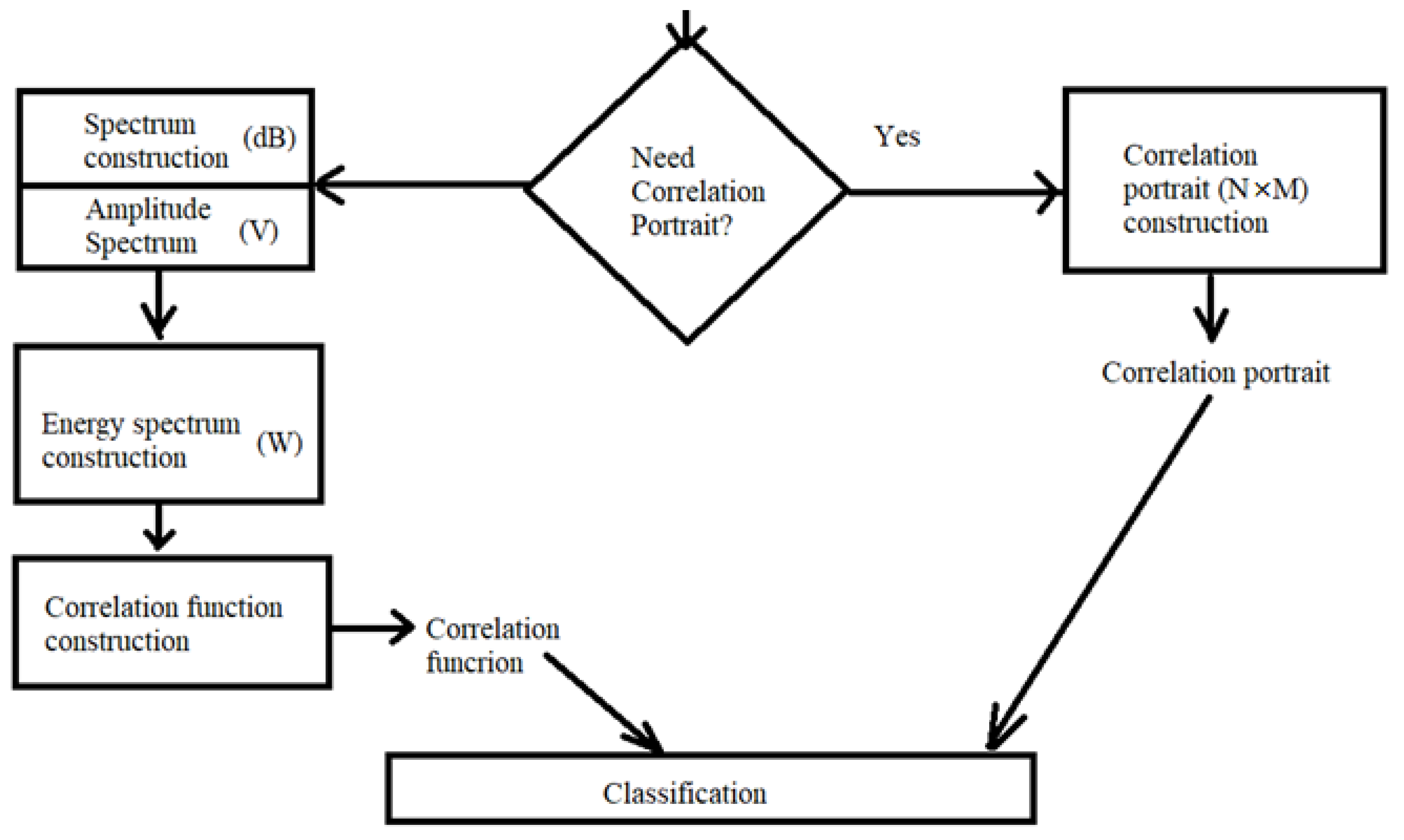
Figure 9 shows the final diagram of the preprocessing of a speech message to prepare for recognition.
In the next section, we will consider the results of comparing the proposed methods for extracting features of speech messages with methods of deep and machine learning.
4. Results
Before proceeding the comparing different algorithms results, it should be noted that the main task is the recognition of a speech message, i.e., the task is classify the message type from 20 studied messages, so classification metrics are used for algorithm evaluation. Another important parameter is the recognition speed, so this parameter is also measured. To be precise, the time taken to recognize one message on average is measured.
Moreover, since there were also machine learning methods among the studied algorithms, the test data consisted of two examples of messages spoken by each speaker, i.e., the data split approach used the classical proportion of 80% by 20% when separating data into training and testing. Thus, the size of the test sample was 400 speech messages, among which there were 20 examples of each class.
Given the balance of training and test data, the accuracy metric was chosen as the main metric.
Table 2 shows the results of efficiency evaluation using the proposed feature extraction methods and known algorithms. As for ANN algorithms, the 1D and 2D Convolutional networks were studied as well as simple recurrent networks and long short term memory (LSTM) networks.
The highest accuracy is provided by the convolutional network after processing the correlation portraits and LSTM networks. It can be explained that long memory is important characteristic for voice messages. However, it is also noticeable that preprocessing in the form of a correlation function also increases the recognition quality.
Table 3 presents the performance results.
The analysis shows that simple algorithms work faster, but they lead to the greatest errors. The best model is the two-dimensional convolutional network. It is almost eight times slower than a recurrent model. However, for pure data, LSTM looks to be best in terms of speed and asset quality. The implementation of quantization of the weights of the convolutional neural network made it possible to reduce the processing time of one message to 831.3 ms.
Finally, we will study the efficiency of the proposed algorithms under the influence of white Gaussian noise. Let q be the ratio of signal variance to noise variance. Table 4 presents the recognition results under noise conditions.
From the results of Table 3 it is clear that the two-dimensional model is the most resistant to intense noise, however, at a noise level 10 times greater than the signal level, the recognition results drop significantly.
It is interesting that traditional machine learning work very badly if the data are noisy. However recurrent structure is more resistance to noise impact. LSTM shows low resistance to noise data. It is possible to use long short term memory networks for processing pure data.
5. Conclusions
Algorithms for the preprocessing of speech messages were proposed to extract features in the problem of recognizing phraseological radio exchange messages. Preprocessing was based on spectral analysis and obtaining correlation functions from the signal spectrum. Building an autocorrelation portrait of a speech message was also proposed. Then, the data were processed by convolution neural networks. This made it possible to increase the recognition accuracy compared to recurrent networks by about 2%. However, in noisy conditions it is not possible to maintain maximum accuracy. Performance approaches 50% at the signal-to-noise ratio q = 0.1. Quantization also ensures the speed of the two-dimensional convolutional network at the level of the recurrent network. The main results of the work are data acquisition and the proposed methods for their preprocessing. Based on the recordings of speech messages and their spectra, it is proposed that correlation functions are obtained so that all classes become increasingly separable. This is confirmed by the results of the study, the increase in accuracy after preprocessing reaches 1–2%. An additional improvement is provided by the use of autocorrelation portraits. In the future, an investigation into how the size of such portraits affects the accuracy is planned. On data in the absence of noise, LSTM networks are preferable, but they turned out to be unstable under the influence of noise. In this regard, the plans for further research include signal filtering.
Funding
This research received no external funding.
Institutional Review Board Statement
Not applicable.
Informed Consent Statement
Not applicable.
Data Availability Statement
Not applicable.
Conflicts of Interest
The authors declare no conflict of interest.
References
- Parekh, D.; Poddar, N.; Rajpurkar, A.; Chahal, M.; Kumar, N.; Joshi, G.P.; Cho, W. A Review on Autonomous Vehicles: Progress, Methods and Challenges. Electronics 2022, 11, 2162. [Google Scholar] [CrossRef]
- Khanum, A.; Lee, C.-Y.; Yang, C.-S. Deep-Learning-Based Network for Lane Following in Autonomous Vehicles. Electronics 2022, 11, 3084. [Google Scholar] [CrossRef]
- Brunelli, M.; Ditta, C.C.; Postorino, M.N. A Framework to Develop Urban Aerial Networks by Using a Digital Twin Approach. Drones 2022, 6, 387. [Google Scholar] [CrossRef]
- Andriyanov, N.; Vasiliev, K. Using Local Objects to Improve Estimation of Mobile Object Coordinates and Smoothing Trajectory of Movement by Autoregression with Multiple Roots. Adv. Intell. Syst. Comput. 2020, 1038, 1014–1025. [Google Scholar] [CrossRef]
- Jarray, R.; Bouallègue, S.; Rezk, H.; Al-Dhaifallah, M. Parallel Multiobjective Multiverse Optimizer for Path Planning of Unmanned Aerial Vehicles in a Dynamic Environment with Moving Obstacles. Drones 2022, 6, 385. [Google Scholar] [CrossRef]
- Andriyanov, N.A. Combining Text and Image Analysis Methods for Solving Multimodal Classification Problems. Pattern Recognit. Image Anal. 2022, 32, 489–494. [Google Scholar] [CrossRef]
- Mukhamadiyev, A.; Khujayarov, I.; Djuraev, O.; Cho, J. Automatic Speech Recognition Method Based on Deep Learning Approaches for Uzbek Language. Sensors 2022, 22, 3683. [Google Scholar] [CrossRef]
- Ramos-Pérez, E.; Alonso-González, P.J.; Núñez-Velázquez, J.J. Multi-Transformer: A New Neural Network-Based Architecture for Forecasting S & P Volatility. Mathematics 2021, 9, 1794. [Google Scholar] [CrossRef]
- Andriyanov, N.; Papakostas, G. Optimization and Benchmarking of Convolutional Networks with Quantization and OpenVINO in Baggage Image Recognition. In Proceedings of the 2022 VIII International Conference on Information Technology and Nanotechnology (ITNT), Samara, Russia, 23–27 May 2022; pp. 1–4. [Google Scholar] [CrossRef]
- Wu, X.; Jin, Y.; Wang, J.; Qian, Q.; Guo, Y. MKD: Mixup-Based Knowledge Distillation for Mandarin End-to-End Speech Recognition. Algorithms 2022, 15, 160. [Google Scholar] [CrossRef]
- Andriyanov, N.; Dementiev, V.; Gladkikh, A. Analysis of the Pattern Recognition Efficiency on Non-Optical Images. In Proceedings of the 2021 Ural Symposium on Biomedical Engineering, Radioelectronics and Information Technology (USBEREIT), Yekaterinburg, Russia, 13–14 May 2021; pp. 0319–0323. [Google Scholar] [CrossRef]
- Rizà Porta, R.; Sterchi, Y.; Schwaninger, A. How Realistic Is Threat Image Projection for X-ray Baggage Screening? Sensors 2022, 22, 2220. [Google Scholar] [CrossRef]
- Ribas, D.; Miguel, A.; Ortega, A.; Lleida, E. Wiener Filter and Deep Neural Networks: A Well-Balanced Pair for Speech Enhancement. Appl. Sci. 2022, 12, 9000. [Google Scholar] [CrossRef]
- Antonetti, A.E.d.S.; Siqueira, L.T.D.; Gobbo, M.P.d.A.; Brasolotto, A.G.; Silverio, K.C.A. Relationship of Cepstral Peak Prominence-Smoothed and Long-Term Average Spectrum with Auditory–Perceptual Analysis. Appl. Sci. 2020, 10, 8598. [Google Scholar] [CrossRef]
- Andriyanov, N.; Andriyanov, D. Intelligent Processing of Voice Messages in Civil Aviation: Message Recognition and the Emotional State of the Speaker Analysis. In Proceedings of the 2021 International Siberian Conference on Control and Communications (SIBCON), Kazan, Russia, 13–15 May 2021; pp. 1–5. [Google Scholar] [CrossRef]
- Andriyanov, N.A. Recognition of radio exchange voice messages in aviation based on correlation analysis. Izv. Samara Sci. Cent. Russ. Acad. Sci. 2021, 23, 91–96. [Google Scholar] [CrossRef]
- LeCun, Y.; Bengio, Y.; Hinton, G. Deep learning. Nature 2015, 521, 436–444. [Google Scholar] [CrossRef]
- Dhouib, A.; Othman, A.; El Ghoul, O.; Khribi, M.K.; Al Sinani, A. Arabic Automatic Speech Recognition: A Systematic Literature Review. Appl. Sci. 2022, 12, 8898. [Google Scholar] [CrossRef]
- Nallasamy, U.; Metze, F.; Schultz, T. Active Learning for Accent Adaptation in Automatic Speech Recognition. In Proceedings of the 2012 IEEE Spoken Language Technology Workshop (SLT), Miami, FL, USA, 2–5 December 2012; pp. 360–365. [Google Scholar]
- Wahyuni, E.S. Arabic Speech Recognition Using MFCC Feature Extraction and ANN Classification. In Proceedings of the 2017 2nd International Conferences on Information Technology, Information Systems and Electrical Engineering (ICITISEE), Yogyakarta, Indonesia, 1–2 November 2017; pp. 22–25. [Google Scholar]
- Trinh Van, L.; Dao Thi Le, T.; Le Xuan, T.; Castelli, E. Emotional Speech Recognition Using Deep Neural Networks. Sensors 2022, 22, 1414. [Google Scholar] [CrossRef]
- Satt, A.; Rozenberg, S.; Hoory, R. Efficient Emotion Recognition from Speech Using Deep Learning on Spectrograms. In Proceedings of the International Speech Communication Association (INTERSPEECH), Stockholm, Sweden, 20–24 August 2017; pp. 1089–1093. [Google Scholar]
- Aksyonov, K.; Antipin, D.; Afanaseva, T.; Kalinin, I.; Evdokimov, I.; Shevchuk, A.; Karavaev, A.; Chiryshev, U.; Talancev, E. Testing of the Speech Recognition Systems Using Russian Language Models. CEUR Workshop Proc. 2018, 2298, 1–7. [Google Scholar]
- Vazhenina, D.; Kipyatkova, I.; Markov, K.; Karpov, A. State-of-the-art speech recognition technologies for Russian language. HCCE’12. In Proceedings of the 2012 Joint International Conference on Human-Centered Computer Environments, Aizu-Wakamatsu, Japan, 8–13 March 2012; pp. 59–63. [Google Scholar] [CrossRef]
- Bagley, S.; Antonov, A.; Meshkov, B.; Sukhanov, A. Statistical Distribution of Words in a Russian Text Collection. In Proceedings of the Dialogue 2009, Bekasovo, Serbia, 27–31 May 2009; pp. 13–18. [Google Scholar]
- Alqadasi, A.M.A.; Sunar, M.S.; Turaev, S.; Abdulghafor, R.; Hj Salam, M.S.; Alashbi, A.A.S.; Salem, A.A.; Ali, M.A.H. Rule-Based Embedded HMMs Phoneme Classification to Improve Qur’anic Recitation Recognition. Electronics 2023, 12, 176. [Google Scholar] [CrossRef]
- Oh, D.; Park, J.-S.; Kim, J.-H.; Jang, G.-J. Hierarchical Phoneme Classification for Improved Speech Recognition. Appl. Sci. 2021, 11, 428. [Google Scholar] [CrossRef]
- Liu, Z.; Huang, Z.; Wang, L.; Zhang, P. A Pronunciation Prior Assisted Vowel Reduction Detection Framework with Multi-Stream Attention Method. Appl. Sci. 2021, 11, 8321. [Google Scholar] [CrossRef]
- Jeon, S.; Kim, M.S. Noise-Robust Multimodal Audio-Visual Speech Recognition System for Speech-Based Interaction Applications. Sensors 2022, 22, 7738. [Google Scholar] [CrossRef] [PubMed]
- Vazhenina, D.; Markov, K. End-to-End Noisy Speech Recognition Using Fourier and Hilbert Spectrum Features. Electronics 2020, 9, 1157. [Google Scholar] [CrossRef]
- Pervaiz, A.; Hussain, F.; Israr, H.; Tahir, M.A.; Raja, F.R.; Baloch, N.K.; Ishmanov, F.; Zikria, Y.B. Incorporating Noise Robustness in Speech Command Recognition by Noise Augmentation of Training Data. Sensors 2020, 20, 2326. [Google Scholar] [CrossRef] [PubMed]
- Andriyanov, N.A.; Andriyanov, D.A. The using of data augmentation in machine learning in image processing tasks in the face of data scarcity. J. Phys. Conf. Ser. 2020, 1661, 012018. [Google Scholar] [CrossRef]
- Box, G.; Jenkins, G.; Reinsel, G. Time Series Analysis; John Wiley & Sons, Inc.: Hoboken, NJ, USA, 2008; p. 755. [Google Scholar]
- Draper, N.R.; Smith, H. Applied Regression Analysis; Wiley: New York, NY, USA, 1966; p. 407. [Google Scholar]
- Zhihua, W.; Yongbo, Z.; Huimin, F. Autoregressive Prediction with Rolling Mechanism for Time Series Forecasting with Small Sample Size. Math. Probl. Eng. 2014, 2014, 572173. [Google Scholar]
- Orzechowski, A.; Bombol, M. Energy Security, Sustainable Development and the Green Bond Market. Energies 2022, 15, 6218. [Google Scholar] [CrossRef]
- Prajakta, S.K. Time series Forecasting using Holt-Winters Exponential Smoothing. Kanwal Rekhi Sch. Inf. Technol. J. 2004, 13, 1–13. [Google Scholar]
- Suyamto, D.; Prasetyo, L.; Setiawan, Y.; Wijaya, A.; Kustiyo, K.; Kartika, T.; Effendi, H.; Permatasari, P. Measuring Similarity of Deforestation Patterns in Time and Space across Differences in Resolution. Geomatics 2021, 1, 464–495. [Google Scholar] [CrossRef]
- Zulifqar, A. Forecasting Drought Using Multilayer Perceptron Artificial Neural Network Model. Adv. Meteorol. 2017, 2017, 5681308. [Google Scholar]
- Sherstinsky, A. Fundamentals of Recurrent Neural Network (RNN) and Long Short-Term Memory (LSTM) Network. Phys. D Nonlinear Phenom. 2020, 404, 132306. [Google Scholar] [CrossRef]
- Andriyanov, N.A.; Dementiev, V.E.; Tashlinskii, A.G. Detection of objects in the images: From likelihood relationships towards scalable and efficient neural networks. Comput. Opt. 2022, 46, 139–159. [Google Scholar] [CrossRef]
- Dua, S.; Kumar, S.S.; Albagory, Y.; Ramalingam, R.; Dumka, A.; Singh, R.; Rashid, M.; Gehlot, A.; Alshamrani, S.S.; AlGhamdi, A.S. Developing a Speech Recognition System for Recognizing Tonal Speech Signals Using a Convolutional Neural Network. Appl. Sci. 2022, 12, 6223. [Google Scholar] [CrossRef]
- Salas-Páez, C.; Quintana-Romero, L.; Mendoza-González, M.A.; Álvarez-García, J. Analysis of Job Transitions in Mexico with Markov Chains in Discrete Time. Mathematics 2022, 10, 1693. [Google Scholar] [CrossRef]
- Yohannes, Y.; Webb, P. Classification and Regression Trees, CART: A User Manual for Identifying Indicators of Vulnerability to Famine and Chronic Food Insecurity; International Food Policy Research Institute: Washington, DC, USA, 1999; p. 59. [Google Scholar]
- Pehlivanoglu, I.V.; Atik, I. Time series forecasting via genetic algorithm for turkish air transport market. J. Aeronaut. Space Technol. 2016, 9, 23–33. [Google Scholar]
- Wenzel, F.; Galy-Fajou, T.; Deutsch, M.; Kloft, M. Bayesian Nonlinear Support Vector Machines for Big Data. In Machine Learning and Knowledge Discovery in Databases: European Conference, ECML PKDD 2017, Skopje, Macedonia, 18–22 September 2017, Proceedings, Part I; Springer: Cham, Switzerland, 2017; pp. 307–322. [Google Scholar]
- Kozionova, A.P.; Pyaita, A.L.; Mokhova, I.I.; Ivanov, Y.P. Algorithm based on the transfer function model and one-class classification for detecting the anomalous state of dams. Inf. Control. Syst. 2015, 6, 10–18. [Google Scholar]
- Timina, I.; Egov, E.; Yarushkina, N.; Kiselev, S. Identification anomalies the time series of metrics of project based on entropy measures. Interact. Syst. Probl. Hum. Comput. Interact. 2017, 1, 246–254. [Google Scholar]
- Woods, J.W.; Dravida, S.; Mediavilla, R. Image Estimation Using Doubly Stochastic Gaussian Random Field Models. Pattern Anal. Mach. Intell. 1987, 9, 245–253. [Google Scholar] [CrossRef]
- Danilov, A.N.; Andriyanov, N.A.; Azanov, P.T. Ensuring the effectiveness of the taxi order service by mathematical modeling and machine learning. J. Phys. Conf. Ser. 2018, 1096, 012188. [Google Scholar] [CrossRef]
- Andriyanov, N.; Dementiev, V.; Tashlinskiy, A. Development and Research of Intellectual Algorithms in Taxi Service Data Processing Based on Machine Learning and Modified K-means Method. In Intelligent Decision Technologies. Smart Innovation, Systems and Technologies; Springer: Singapore, 2022; Volume 309, pp. 183–192. [Google Scholar] [CrossRef]
- Armer, A.I. Modeling and Recognition of Speech Signals Against the Background of Intense Interference. Ph.D. Thesis, Ulyanovsk State Technical University, Ulyanovsk, Russia, 20 June 2006; pp. 1–190. [Google Scholar]
- Krasheninnikov, V.R.; Lebedeva, E.Y.; Kapyrin, V.K. Variation of the boundaries of speech commands to improve the recognition of speech commands by their cross-correlation portraits. In Proceedings of the Samara Scientific Center of the Russian Academy of Sciences, Samara, Russia, 20–21 November 2013; Volume 15, pp. 928–930. [Google Scholar]
- Ayvaz, U.; Guruler, H.; Khan, F.; Ahmed, N.; Whangbo, T.; Abdusalomov, A. Automatic Speaker Recognition Using Mel-Frequency Cepstral Coefficients Through Machine Learning. Comput. Mater. Contin. 2022, 71, 5511–5521. [Google Scholar] [CrossRef]
- Khan, F.; Tarimer, I.; Alwageed, H.S.; Karadağ, B.C.; Fayaz, M.; Abdusalomov, A.B.; Cho, Y.-I. Effect of Feature Selection on the Accuracy of Music Popularity Classification Using Machine Learning Algorithms. Electronics 2022, 11, 3518. [Google Scholar] [CrossRef]
- Audacity. Available online: https://www.audacityteam.org/ (accessed on 11 January 2023).
Figure 1.
Time series of studied radio messages.
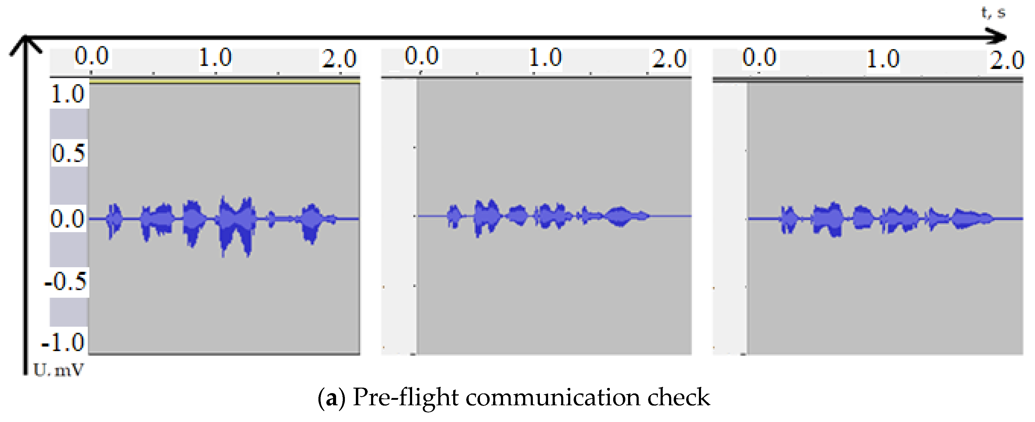
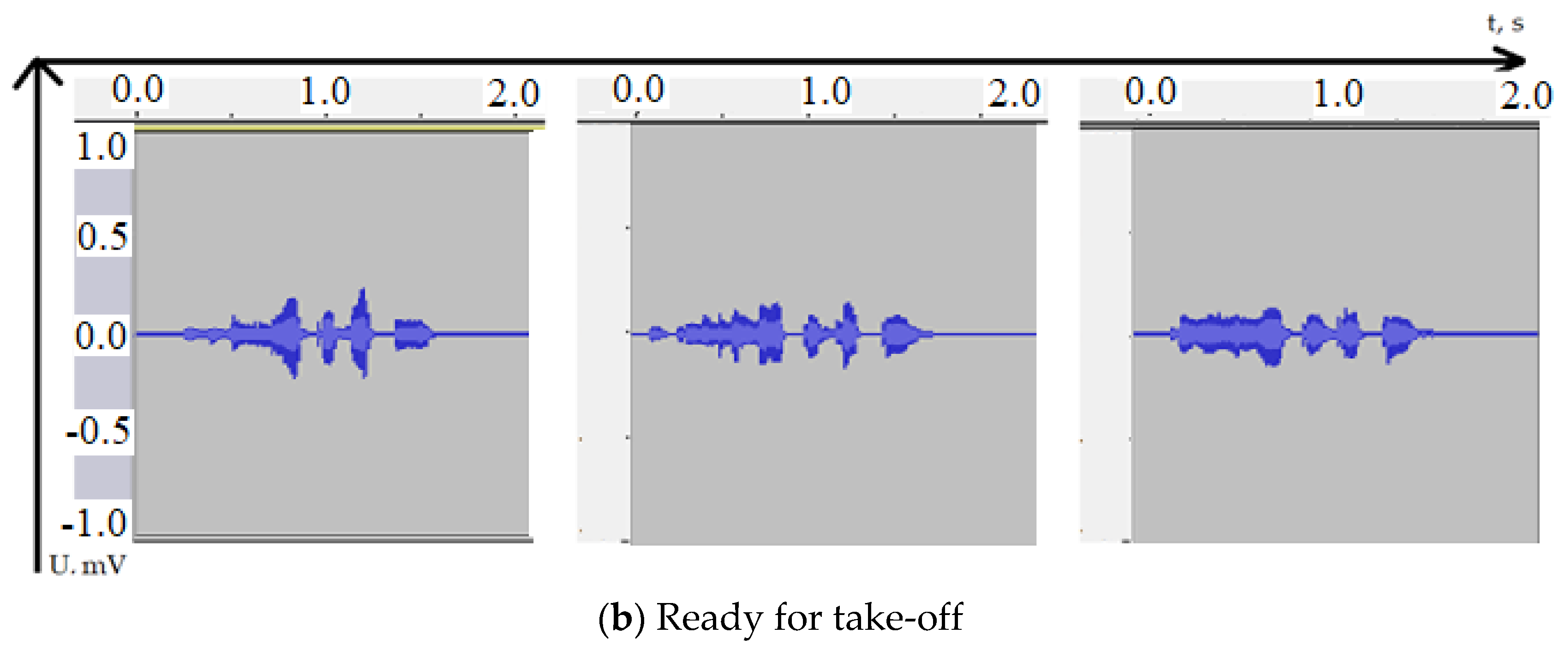
Figure 2.
The spectrum of the studied radio messages.
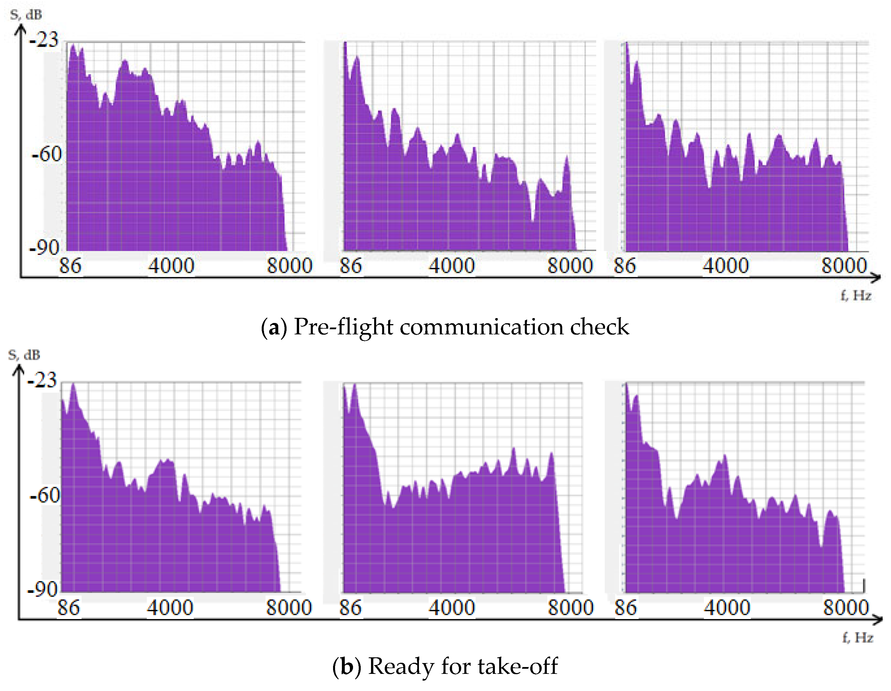
Figure 3.
Spectra of various messages after averaging.
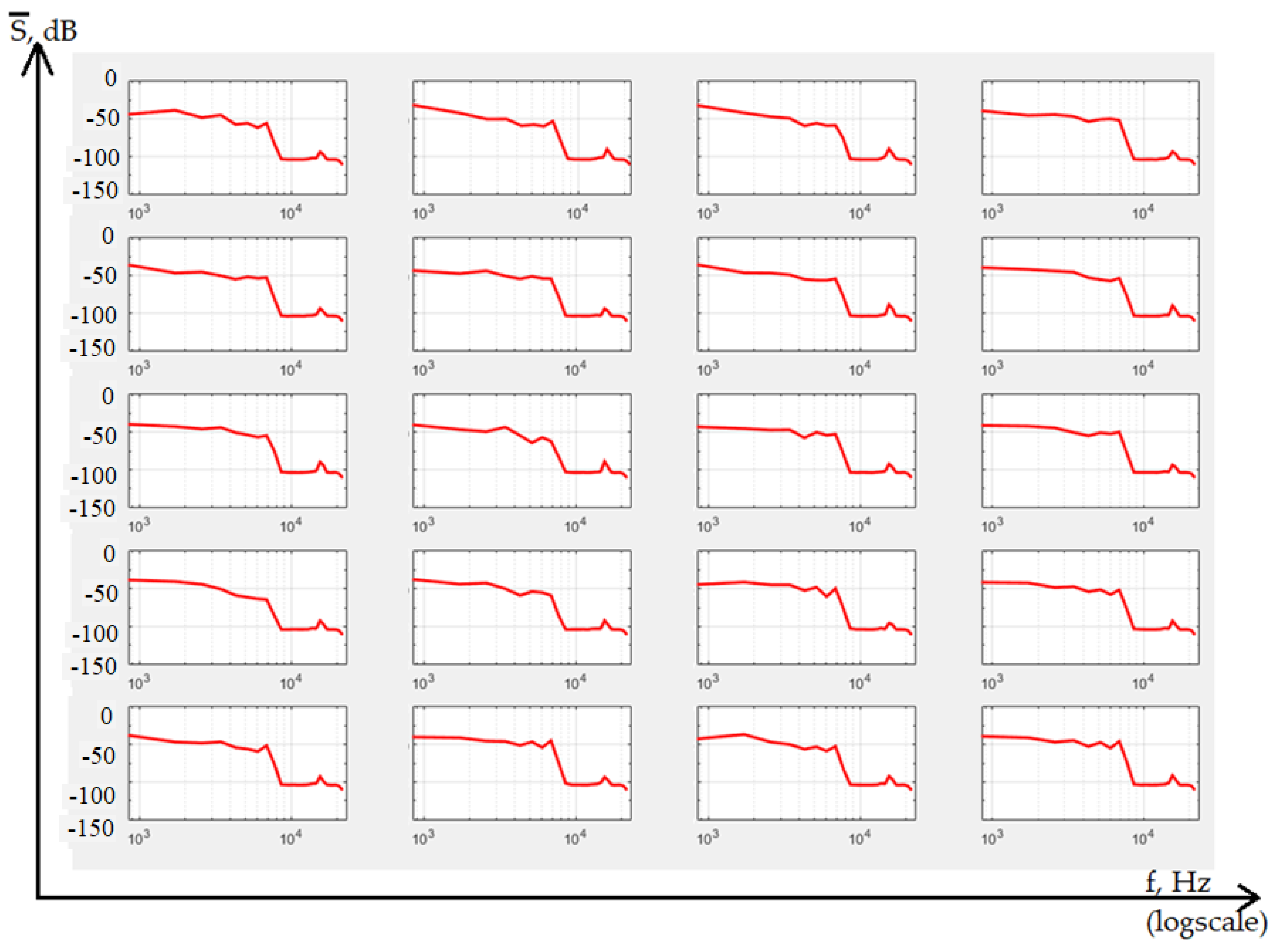
Figure 4.
An example of spectra of absolute voltage values after averaging.
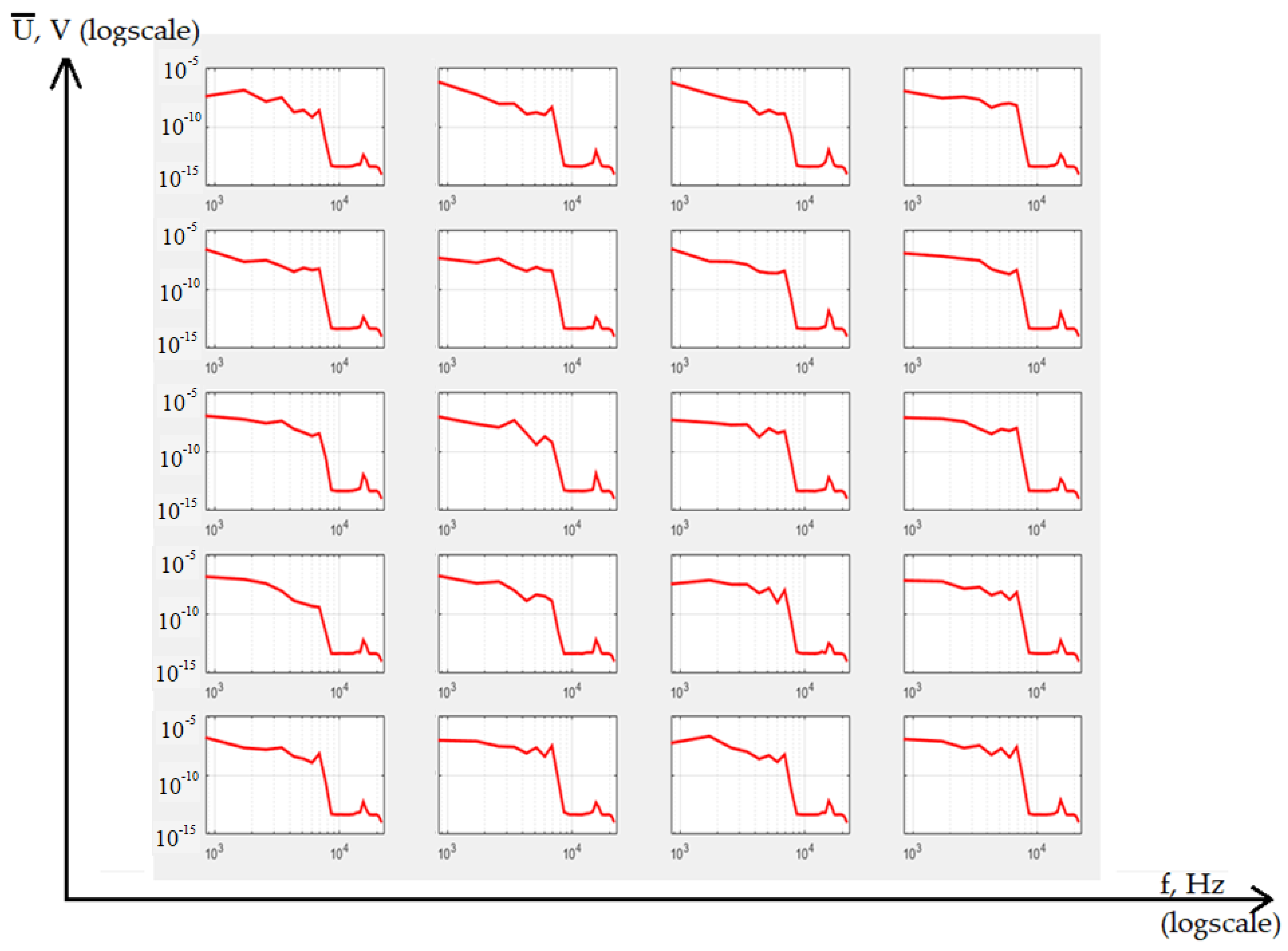
Figure 5.
Examples of the radio exchange messages energy spectrum.
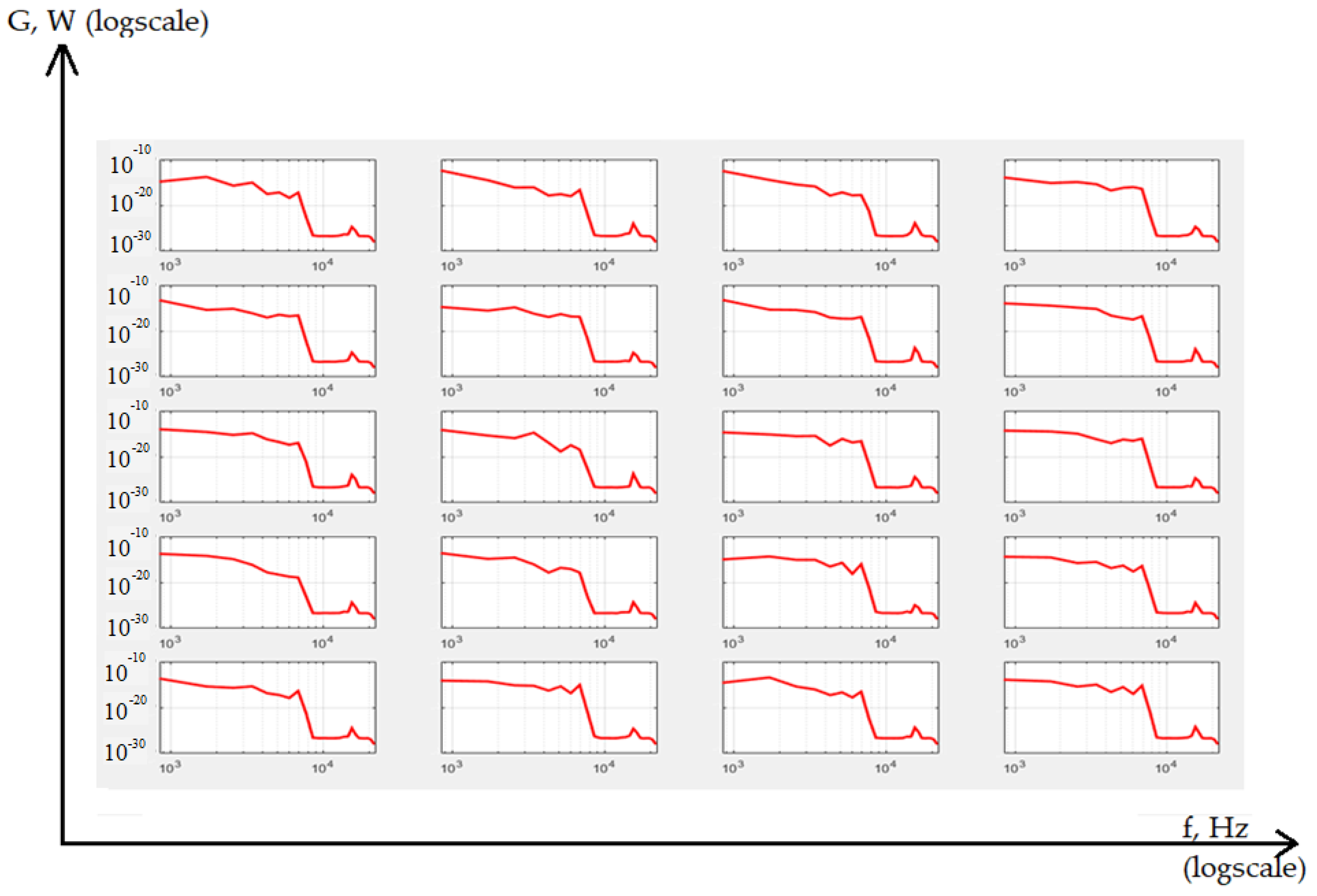
Figure 6.
Examples of radio exchange messages correlation functions.
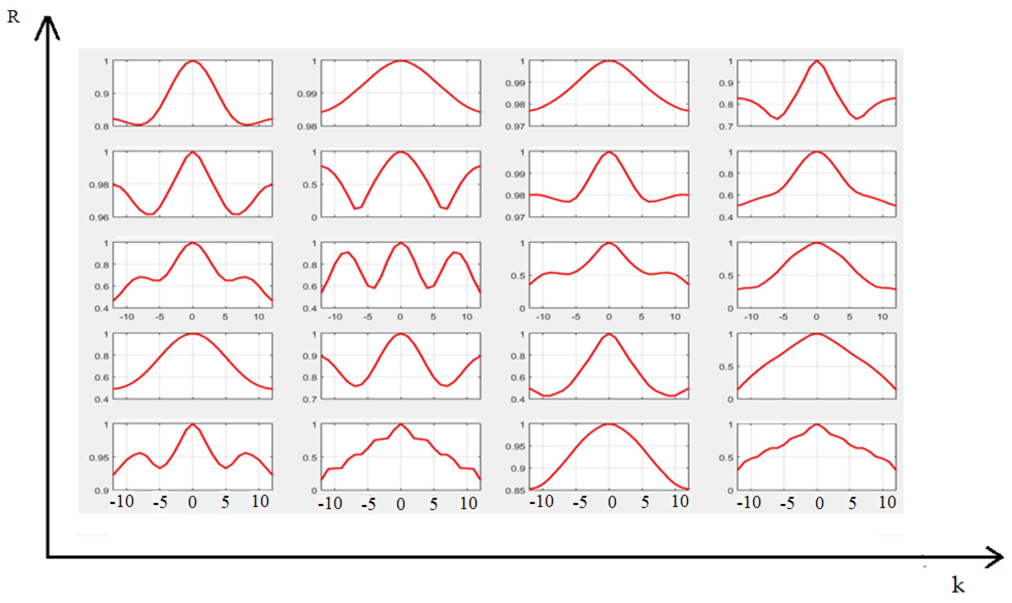
Figure 7.
Autocorrelation portraits for the phrase “Pre-flight check”.
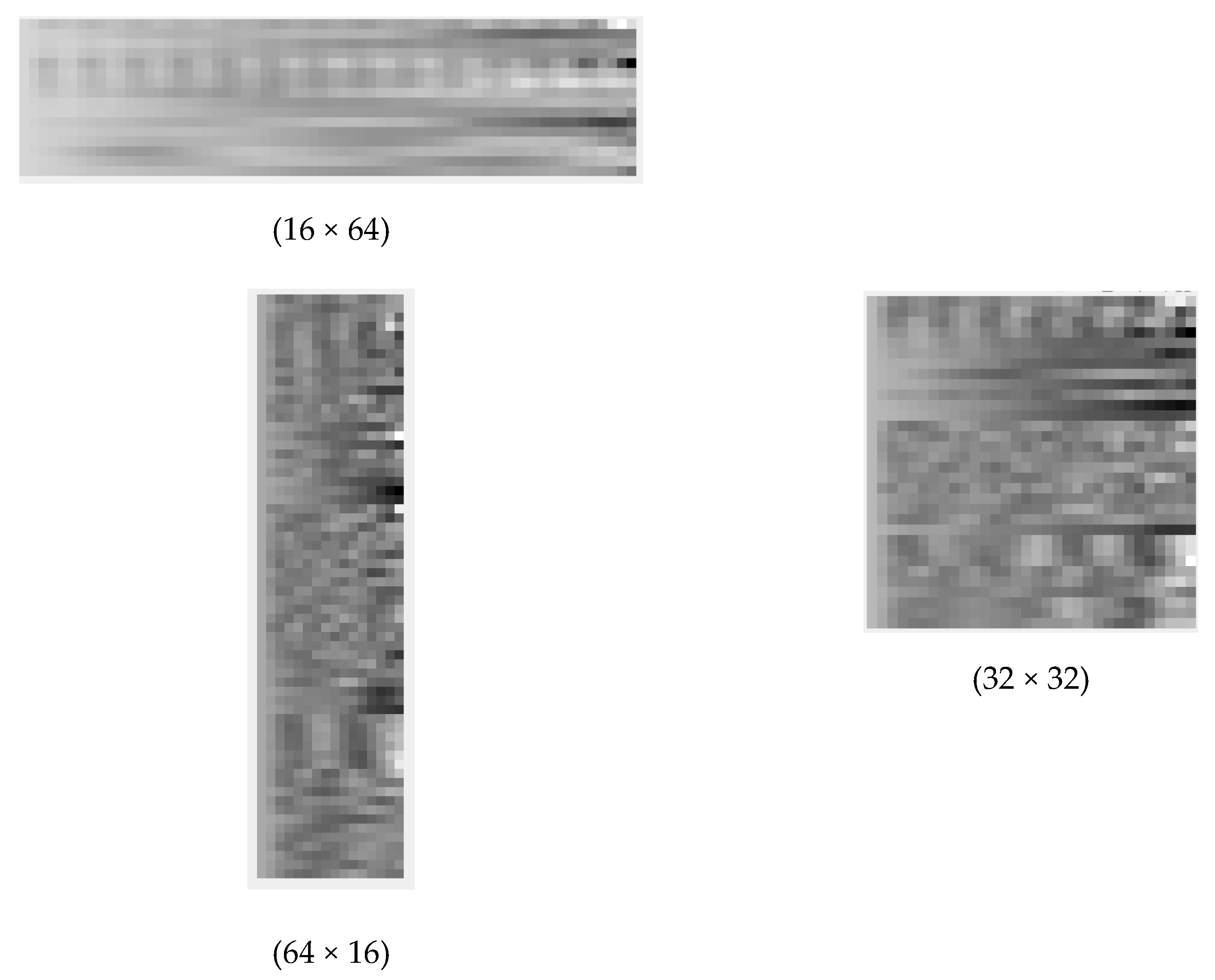
Figure 8.
Comparison of autocorrelation portraits.
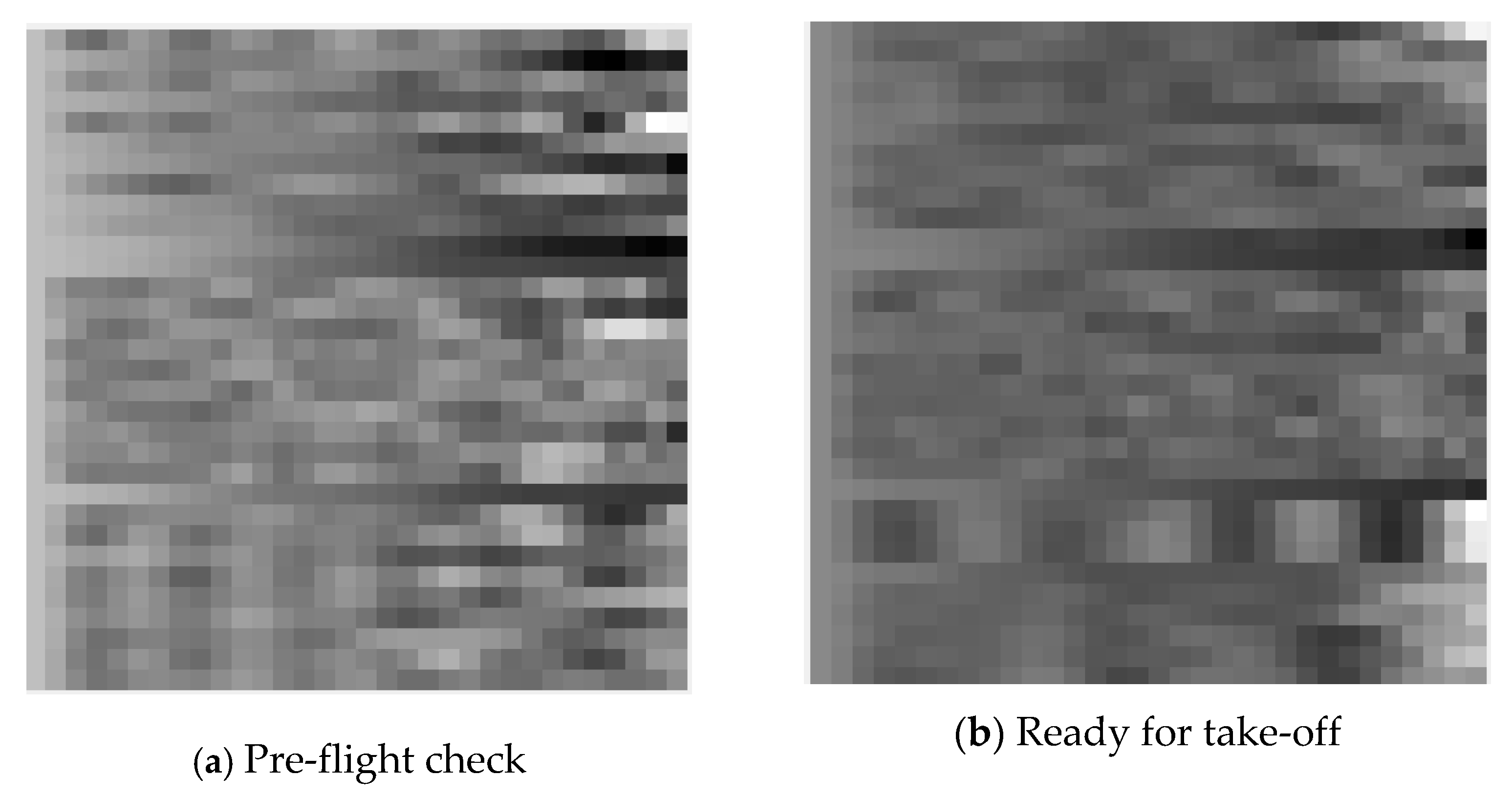
Figure 9.
Comparison of autocorrelation portraits.

Table 1.
Representation and processing of time series.
| Algorithm | Pros | Cons |
|---|---|---|
| Regression models | Simplicity, high level of knowledge | Narrow scope, strong retrainability, the need for combined time series |
| Autoregressive models | Taking into account the internal connections of the signal, the developed mathematical apparatus | Impossibility of describing signals with a complex structure |
| Exponential smoothing models | Smoothing out slowly changing signals in noisy environments | Inability to describe speech signals with high accuracy |
| Models on the most similar pattern | Adequate description of normal data | Impossible to represent heterogeneous data |
| Artificial neural networks | Flexible parameter setting, high accuracy | High computational costs, high model complexity, low stability |
| Markov chains | Simplicity, taking into account the dynamics of random processes | Too short memory for describing speech signals |
| Classification-regression trees | Good interpretability of results, sufficiently high accuracy | Strong retrainability of models |
| Genetic algorithm | Wide application, relatively high efficiency | High computational cost |
| Support vector machine | Working with non-linear connections, flexible settings | Necessity of preprocessing, searching for parameters |
| Transfer function | Adequate description of complex data | High computational cost, low performance |
| Fuzzy logic | Universality of approach, probabilistic estimates | Inability to accurately describe speech messages, complexity of mathematical analysis |
| Doubly stochastic models | Ability to describe inhomogeneous and non-stationary signals | Difficulty in identifying model parameters |
Table 2.
Recognition accuracy.
| Algorithm | Accuracy |
|---|---|
| Decision tree (depth 10) | 92.50% |
| Support vector machine | 93.50% |
| Fully connected neural network (3 layers, 20-20-20 neurons) | 94.25% |
| Recurrent neural network (recurrent layer 24 neurons) | 95.50% |
| Long Short Term Memory Network (LSTM layer 24 neurons) | 96.00% |
| 1D Convolutional Neural Network (16 filters) | 94.00% |
| Fully Connected Network based on correlation function | 96.50% |
| Recurrent network based on correlation function | 97.25% |
| LSTM network based on correlation function | 97.50% |
| Convolutional network based on correlation function | 95.75% |
| Convolutional network based on correlation portrait | 97.50% |
Table 3.
Recognition time.
| Algorithm | Processing Time, ms |
|---|---|
| Decision tree (depth 10) | 2.35 |
| Support vector machine | 8.94 |
| Fully connected neural network (3 layers, 20-20-20 neurons) | 246.80 |
| Recurrent neural network (recurrent layer 24 neurons) | 320.55 |
| Long Short Term Memory Network (LSTM layer 24 neurons) | 654.35 |
| 1D Convolutional Neural Network (16 filters) | 806.20 |
| Fully Connected network based on correlation function | 246.80 + 18.40 |
| Recurrent network based on correlation function | 320.55 + 18.40 |
| LSTM network based on correlation function | 654.35 + 18.40 |
| Convolutional network based on correlation function | 806.20 + 18.40 |
| Convolutional network based on correlation portrait | 2325.62 |
Table 4.
Noisy messages recognition.
| Algorithm | q = 0.1 | q = 1 | q = 10 |
|---|---|---|---|
| Decision tree (depth 10) | 35.75% | 78.25% | 92.50% |
| Support vector machine | 37.00% | 75.50% | 93.25% |
| Fully connected neural network (3 layers, 20-20-20 neurons) | 45.75% | 87.25% | 94.25% |
| Recurrent neural network (recurrent layer 24 neurons) | 54.25% | 83.75% | 95.50% |
| Long short term memory network (LSTM layer 24 neurons) | 49.75% | 80.50% | 96.00% |
| 1D convolutional neural network (16 filters) | 39.50% | 86.25% | 94.00% |
| Fully connected network based on correlation function | 57.25% | 92.25% | 96.50% |
| Recurrent network based on correlation function | 59.00% | 93.25% | 97.25% |
| LSTM network based on correlation function | 52.25% | 94.00% | 97.50% |
| Convolutional network based on correlation function | 51.00% | 91.00% | 95.75% |
| Convolutional network based on correlation portrait | 53.25% | 96.75% | 97.50% |
Disclaimer/Publisher’s Note: The statements, opinions and data contained in all publications are solely those of the individual author(s) and contributor(s) and not of MDPI and/or the editor(s). MDPI and/or the editor(s) disclaim responsibility for any injury to people or property resulting from any ideas, methods, instructions or products referred to in the content. |
© 2023 by the author. Licensee MDPI, Basel, Switzerland. This article is an open access article distributed under the terms and conditions of the Creative Commons Attribution (CC BY) license (https://creativecommons.org/licenses/by/4.0/).
Share and Cite
MDPI and ACS Style
Andriyanov, N. The Use of Correlation Features in the Problem of Speech Recognition. Algorithms 2023, 16, 90. https://doi.org/10.3390/a16020090
AMA Style
Andriyanov N. The Use of Correlation Features in the Problem of Speech Recognition. Algorithms. 2023; 16(2):90. https://doi.org/10.3390/a16020090
Chicago/Turabian StyleAndriyanov, Nikita. 2023. "The Use of Correlation Features in the Problem of Speech Recognition" Algorithms 16, no. 2: 90. https://doi.org/10.3390/a16020090
Note that from the first issue of 2016, this journal uses article numbers instead of page numbers. See further details here.